Three-Dimensional Limited-Memory BFGS Inversion of Magnetic Data Based on a Multiplicative Objective Function

Abstract

At present, the traditional magnetic three-dimensional inversion method has been fully developed and is widely used. Magnetic exploration is a kind of geophysical exploration method that uses the magnetic field changes (magnetic anomalies) caused by the magnetic differences between various rocks in the crust to find useful mineral resources and study the underground structure. Traditional magnetic three-dimensional inversion is relatively inefficient. Moreover, the traditional additive objective function (data fitting difference term plus regularization term and logarithmic obstacle term), which causes the regularization factor selection to be more complicated, is implemented in this method. Therefore, it is necessary to establish a new efficient three-dimensional magnetic inversion algorithm and optimize the selection of regularization factors. In this paper, based on the limited-memory BFGS (L-BFGS) method, the three-dimensional magnetic inversion of a multiplicative objective function is realized. The inversion test is conducted in this paper using both theoretical synthesis data and measured data. The results demonstrate that the limited-memory BFGS method significantly enhances the inversion efficiency and yields superior inversion outcomes compared to traditional magnetic three-dimensional inversion methods. Additionally, the multiplicative objective function-based three-dimensional magnetic inversion method simplifies the process of selecting weight factors for regularization terms.

1. Introduction

Magnetic exploration is a kind of geophysical exploration method that uses the magnetic field changes (magnetic anomalies) caused by the magnetic differences between various rocks (ore) in the crust to find useful mineral resources and study the underground structure [1,2,3]. Magnetic prospecting is widely used to search for useful mineral resources [4,5,6]. In the late 1950s and early 1960s, the Soviet Union and the United States began ocean magnetic surveys, and continental drift theory entered a new historical stage. Since the 1980s in China, the rapid development of high-precision magnetometers has significantly advanced magnetic exploration [7].

The regularized inversion algorithm based on the logarithmic barrier method [8,9] proposed by Li and Oldenburg in 1996 and 2003 is mostly used in the three-dimensional inversion of magnetic methods [10]. The logarithmic barrier term increases the complexity of retrieving the objective function. In the direct current inversion method, the logarithm of the model resistivity is usually adopted to avoid negative values of the model parameters. Based on the same idea, the logarithm of the magnetic susceptibility is used, and the inversion can then be carried out. At the same time, the efficiency of the three-dimensional inversion of magnetic methods based on the logarithmic barrier method is low. Currently, the limited-memory BFGS (L-BFGS) method has been mostly applied to the inversion of various geophysical methods [11,12]. The limited-memory BFGS (L-BFGS) method has good stability, requires less memory, performs only one quasi-forward simulation and is fast and efficient.

In the past, the objective function used in the inversion of magnetic methods was generally an additive objective function. One problem faced by this type of objective function in the inversion is that regularization factors need to be selected, and the selection of regularization factors can only be carried out according to experience or repeated inversion trial calculations, resulting in a low inversion efficiency and requiring more inversion time. With the further development of inversion at home and abroad, the objective function has been further developed. In 2002 and 2009, Van den Berg et al. proposed a contrast source inversion method based on the multiplicative objective function [13,14,15]. This method has been applied to large-scale electromagnetic inversion and log inversion [16]. The multiplicative objective function has been applied to three-dimensional inversion via the resistivity method, and good inversion results have been obtained. [17] The advantage of this kind of objective function is that it automatically adjusts the weight between the data fitting difference term and the regularization term in the inversion iteration process, and it does not need to repeatedly select regularization factors, which provides great convenience for inversion. At present, the three-dimensional inversion of the resistivity method based on the multiplicative objective function has been achieved in China, but the multiplicative objective function in other geophysical methods has not been applied.

In this paper, the logarithmic magnetic susceptibility method, which eliminates the logarithmic barrier in the objective function and simplifies the objective function, is adopted. The limited-memory BFGS (L-BFGS) method is used to achieve three-dimensional magnetic inversion based on the multiplicative objective function. In this paper, the synthetic data of single prism and oblique prism anomalous body models are used for inversion, and the measured data are also used for inversion. The feasibility and effectiveness of magnetic inversion based on multiplicative objective function are verified, and a new idea is provided for selecting the weights between data items and model items.

2. Forward and Inversion Theory

2.1. Three Dimensional Forward Modelling of the Magnetic Method

The forward model studied in this paper does not consider remanence and demagnetization, so forward inference can therefore be regarded as an analytic solution problem. We divided the subsurface into cubic units of the same size and different magnetic susceptibilities and then calculated the magnetic anomalies caused by the unit at a certain observation point. The total magnetic anomaly at the measuring point was obtained by means of the summation of the magnetic anomaly caused by all the cube elements at the measuring point position.

The parameters of a single cube unit are shown in Figure 1. Its central coordinates are set to (${\mathrm{x}}_0$,${\mathrm{y}}_0$,${\mathrm{z}}_0$); the length, width and height of the cube unit are a, b and c, respectively; and the observation point is s (x, y, z).

The magnetic anomaly ΔT caused by the anomalous body element at the observation point s (x, y, z) is [18]:

$$\begin{array}{cc}\hfill \mathsf{\Delta }\mathrm{T}\left(x,y,z\right)& =G^{\mathrm{mag}}\kappa \hfill \\ & =\frac{{\mathsf{\mu }}_0}{4\mathsf{\pi }}\kappa \left\{k_{1}ln\right[r+(\xi -x)]+k_{2}ln[r+(\eta -y)]+k_{3}ln[r+(\xi -z)]\hfill \\ & +k_{4}arctan\frac{(\xi -x)(\eta -y)}{{(\xi -x)}^2+r(\xi -z)+{(\xi -z)}^2}\hfill \\ & +k_{5}arctan\frac{(\xi -x)(\eta -y)}{{(\xi -y)}^2+r(\xi -z)+{(\xi -z)}^2}\hfill \\ & +k_{6}arctan\frac{\left(\xi -x\right)\left(\eta -y\right)}{r\left(\xi -z\right)}\}{|}_{x_0-\frac{a}{2}}^{x_0+\frac{a}{2}}{|}_{y_0-\frac{b}{2}}^{y_0+\frac{b}{2}}{|}_{z_0-\frac{c}{2}}^{z_0+\frac{c}{2}} ,\hfill \end{array}$$

(1)

where $\kappa$ is the magnetic susceptibility matrix of the rectangular element, ${\mathsf{\mu }}_0$ is the vacuum permeability, $G$^mag is the Jacobian matrix, and a, b, and c are the lengths of the cuboid in the xyz direction.

$$\begin{gathered} r=\sqrt{{\left(\xi -x\right)}^2+{\left(\xi -y\right)}^2+{\left(\xi -z\right)}^2}, \\ {k}_1=hN+nM,k_2=lN+nL,k_3=lM+hl,k_4=lL,k_5=hM,k_6=-nN; \\ l=cos{I}_{0}cos{A}_0,h=cos{I}_{0}sin{A}_0,n=sin{I}_0; \\ L=cosIcosA,M=cosIsinA,N=sinI; \end{gathered}$$

(2)

where $l$, h, n, L, M and N are the direction cosines of the geomagnetic field and the total magnetization intensity, respectively; $I_0$, $A_0$, $I$ and $A$ are the inclination angles of the geomagnetic field and the total magnetization and the deviation angles relative to the X-axis, respectively; and $G$^mag is the kernel function of the magnetic anomaly.

Because the magnetic outlier at measuring point s is the superposition of the magnetic outlier generated by all underground rectangular units at the point, the magnetic outlier at measuring point s is calculated using the following formula:

$$\mathsf{\Delta }{T}_i={\sum }_{j=1}^{j=M}{G}_{ij}^{mag}{\kappa }_j,$$

(3)

where $\mathsf{\Delta }{T}_i$ is the magnetic anomaly at observation point i, ${\kappa }_j$ is the magnetic susceptibility of the Jth model element, and $G_{ij}^{mag}$ is the kernel function corresponding to rectangular element j at observation point i.

The three-dimensional forward modeling of magnetic methods can be regarded as the problem of obtaining the abnormal data $\mathsf{\Delta }T$ from magnetic methods by using the kernel G matrix and the magnetic susceptibility of the model vector. The forward mapping to the global inversion formula is a large formula. It can be simplified as follows:

$$d=Gm,$$

(4)

representing the process of obtaining the data result d by using the G matrix and model vector m.

2.2. Magnetic Three-Dimensional Inversion

2.2.1. Traditional Magnetic Three-Dimensional Inversion

Inversion is the process of using the observed data of known fields to solve the geophysical parameters of the corresponding underground geological model. In solving the inversion problem, it is generally an additive objective function, but this objective function needs to determine the weight factor of the regularization term according to experience or numerical experiments, which has a great influence on the inversion efficiency.

In the conventional magnetic method of three-dimensional inversion, the logarithmic obstacle method is often used because of the possibility of negative inversion results. The objective function of traditional magnetic inversion is shown in Equation (1), and the logarithmic obstacle term is the third term, which also needs to determine the weight factor. The addition of this term makes the inversion objective function more complicated, and the efficiency of the traditional magnetic method of three-dimensional inversion is low. Moreover, the time utilization is low.

$$\Phi \left(m\right)={\Phi }_d+\mathsf{\lambda }{\Phi }_m+2\mathsf{\mu }\sum _{j=1}^{M}log\left(m_j\right),$$

(5)

$${\Phi }_d={\left(d-Gm\right)}^T{C}_d^{-1}\left(d-Gm\right),$$

(6)

$${\Phi }_{m_1}={\left(m-m_{pri}\right)}^T{C}_m^{-1}\left(m-m_{pri}\right),$$

(7)

where ${\Phi }_d$ is the data term, ${\Phi }_{m_1}$ is the model term, $\sum _{j=1}^{M}log\left(m_j\right)$ is the logarithmic barrier term, $m$ is the permeability $\kappa$, $m_{pri}$ is the prior model vector, G is the kernel function matrix, $C_m$ is the model covariance matrix, and $C_d$ is the data covariance matrix, T is the transpose operation.

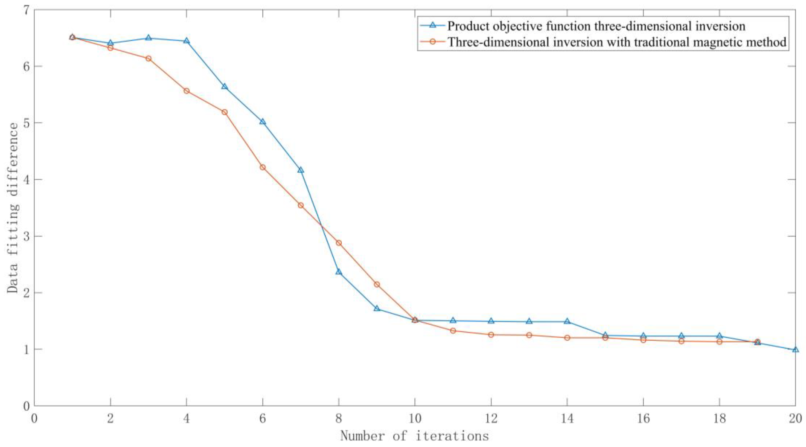
2.2.2. Three-Dimensional Limited-Memory BFGS Inversion Using a Magnetic Method Based on a Multiplicative Objective Function

In this paper, a three-dimensional limited-memory BFGS (L-BFGS) inversion method based on the multiplicative objective function is proposed. This inversion method uses the log-barrier term omitted by the logarithm of model terms, while the multiplicative objective function eliminates the problem of regularization factor selection required by the traditional inversion method. At the same time, the limited-memory BFGS method has a relatively high inversion efficiency.

The objective function of the three-dimensional finite memory quasi-Newtonian inversion by the magnetic method based on the multiplicative objective function is [17]:

$$\Phi \left(m\right)={\Phi }_d\times {\Phi }_{m_2},$$

(8)

$${\Phi }_d={\left(d-Gm\right)}^T{C}_d^{-1}\left(d-Gm\right),$$

(9)

$${\Phi }_{m_2}={\left(m-m_{pri}\right)}^T{C}_m^{-1}\left(m-m_{pri}\right)+\mathsf{\delta },$$

(10)

where ${\Phi }_d$ is the data item, ${\Phi }_{m_2}$ is the model item, $m$ is the permeability $\kappa$, $m_{pri}$ is the prior model vector, G is the kernel function matrix, $C_m$ is the model covariance matrix, and $C_d$ is the data covariance matrix, T is the transpose operation.

The gradient of the objective function is:

$$\psi ={\Phi }_d\times 2C_m^{-1}\left(m-m_{pri}\right)+2C_d^{-1}{G}^T\left(d-Gm\right)\times {\Phi }_{m_2},$$

(11)

where $G^T$ is the transpose of the kernel matrix.

In addition, $\mathsf{\delta }$ in Equation (10) is a constant. To prevent the first inversion of the model term being 0, the objective function is set to 0, resulting in inversion failure.

The method for selecting the constant δ [19] is as follows:

$$\mathsf{\delta }=\sqrt{\frac{\mathrm{N}}{∆\mathrm{V}}} ,$$

(12)

where N is the total number of observed data and $∆\mathrm{V}$ is the average volume of grid division units. In this paper, the uniform mesh is divided, so $∆\mathrm{V}$ is the volume of any cube unit.

L-BFGS uses the objective function gradient of the first (3–20) iterations to approximate the Hessian matrix, which is more efficient and faster than the BFGS and Gauss-Newton methods.

The L-BFGS inversion procedure is as follows:

1.

Determine the initial inversion model, set the maximum number of inversion iterations and the minimum fitting difference, calculate the model item and add the constant value, and carry out depth weighting on the initial model;

2.

Take the natural logarithm of the initial model $m$ and $m_{pri}$;

3.

Calculate the objective function $\Phi$ and the gradient $\psi$;

4.

Calculate the inverse matrix ${\left[H_k\right]}^{-1}$ and the quasi-Newtonian direction $p_k=-{\left[H_k\right]}^{-1}\psi$;

5.

Set the initial step size, and perform a linear search from the initial step size to find the relative best iteration step size $\alpha$;

6.

Update the inversion model $m_{k+1}=m_k+\alpha p_k$ by the determined iteration step size and quasi-Newtonian direction;

7.

Transform the updated models $m$ and $m_{pri}$ using the exponential e;

8.

Determine whether the data fitting difference of the current model is less than the set minimum fitting difference. If it is less, the iteration is stopped, and the depth-weighted inverse transformation is performed on the obtained model $m$; otherwise, the third step is performed again, and the iteration is continued.

The calculation formula of the Hessian matrix for each iteration is:

$${\left[H_k\right]}^{-1}=\left(I-{\rho }_{k-1}{s}_{k-1}{y}_{k-1}^T\right)H_{k-1}^{-1}\left(I-{\rho }_{k-1}{y}_{k-1}{s}_{k-1}^T\right)+{\rho }_{k-1}{s}_{k-1}{s}_{k-1}^T,$$

(13)

where $I$ is the identity matrix, and the ${\rho }_{k-1}$, $s_{k-1}$, and $y_{k-1}$ calculation formulas are:

$${\rho }_{k-1}=\frac{1}{y_{k-1}^T{s}_{k-1}},$$

(14)

$$s_{k-1}={\psi }_k-{\psi }_{k-1},$$

(15)

$$y_{k-1}=m_k-m_{k-1}.$$

(16)

The linear search for the best iteration step must meet the strong wolf condition to ensure that the obtained step size can make the iteration stable, convergent and efficient. The strong wolf condition is:

$${\Phi }_{k+1}\le {\Phi }_k+{\mathrm{c}}_1\alpha {\psi }_k^T{p}_k,$$

(17)

$${|\psi }_{k+1}^T{p}_k\left|\le {\mathrm{c}}_2{|\psi }_k^T{p}_k\right|,$$

(18)

where the constant ${\mathrm{c}}_1$ is generally 0.0001 and the constant ${\mathrm{c}}_2$ is generally 0.9.

The initial step size of the first and subsequent iterations of the inversion is selected as follows:

$${\alpha }_1=\frac{\mathrm{p}}{{\parallel \psi \parallel }_2},$$

(19)

$${\alpha }_{\mathrm{2,3}\dots }=1,$$

(20)

where ${\alpha }_1$ is the initial step of the first iteration, ${\alpha }_{\mathrm{2,3}\dots }$ is the initial step of subsequent iterations, and the most appropriate value of p ranges from 5 to 15.

In addition, the termination condition of the inversion is that the data fitting difference is less than the predefined minimum fitting difference or that the number of iterations reaches the set value. The formula for calculating the data fitting difference (RMS) is as follows:

$$RMS=\sqrt{\frac{{\left(d-Gm\right)}^T{C}_d^{-1}\left(d-Gm\right)}{N}},$$

(21)

where N is the total number of observed data.

3. Example of Theoretical Model Synthesis

Based on the above theoretical methods, we develop a three-dimensional magnetic inversion algorithm based on the multiplicative objective function and limited-memory BFGS (L-BFGS) method. To verify the validity and feasibility of the inversion algorithm, two magnetic susceptibility model examples are designed for analysis. In this paper, the traditional magnetic three-dimensional inversion and the magnetic three-dimensional limited-memory BFGS inversion based on the multiplicative objective function are calculated under the same conditions, and the computing environment is a personal computer equipped with Lenovo (Beijing, China) M2000(Inter(R)Core(TM)i5-3470 [email protected] GHz CPU and 24 GB memory).

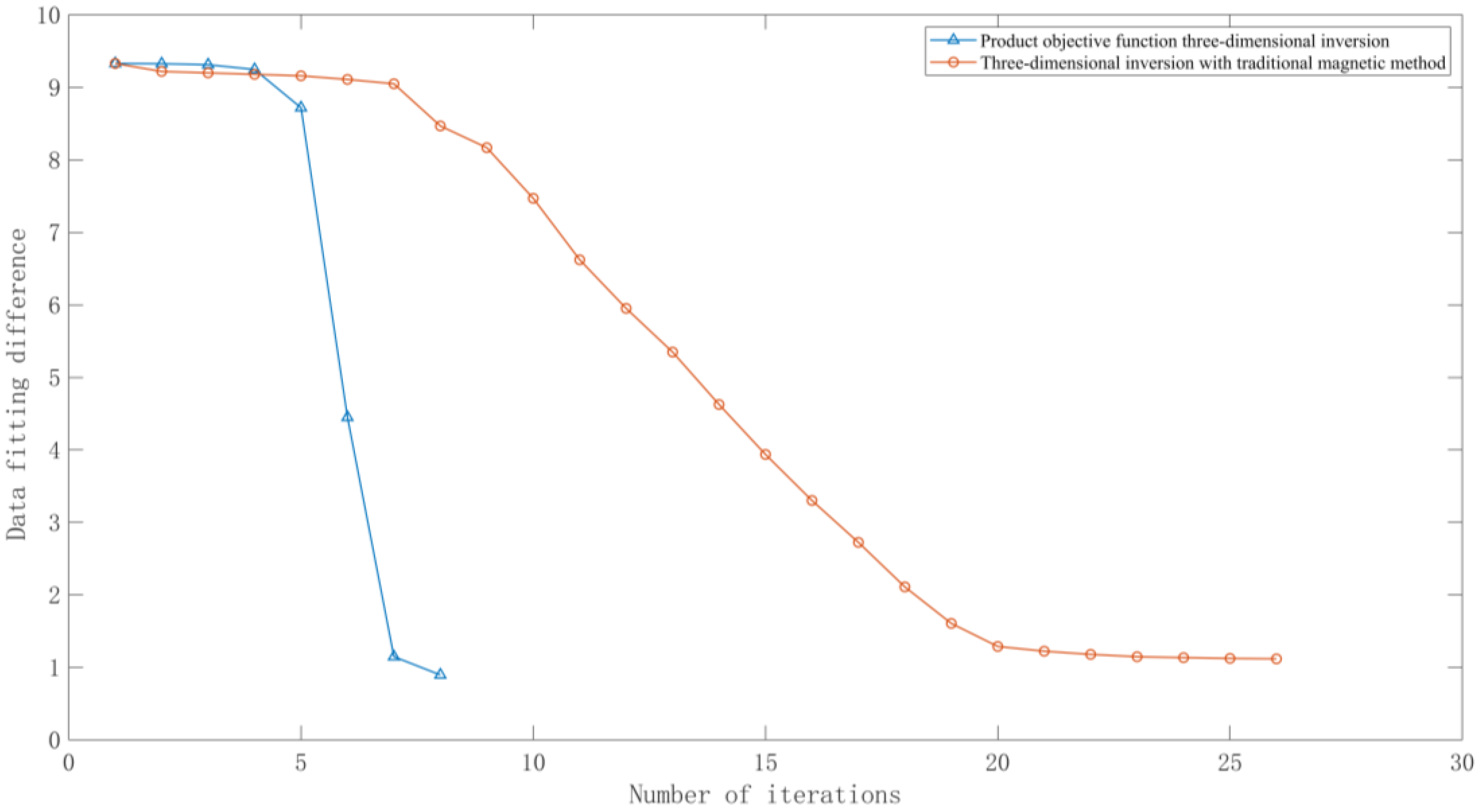
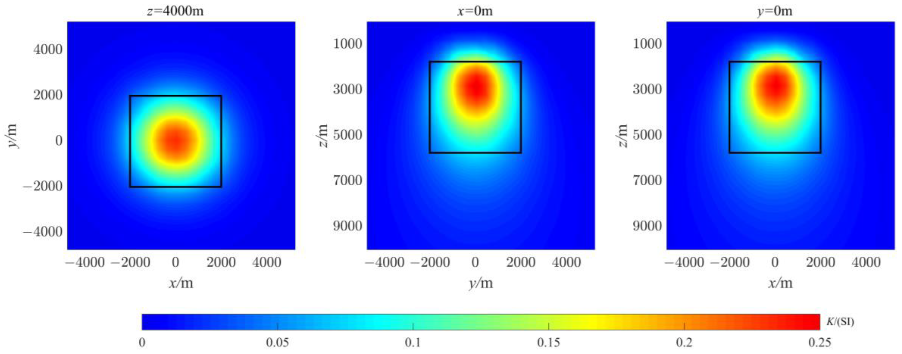
3.1. Example of Single Prism Synthesis

As shown in Figure 2, a single prism with a size of 4 km × 4 km × 4 km is placed underground, and the top is buried at a depth of 2 km. The inversion area is set to 10 km × 10 km × 10 km, and it is divided into 9261 cube units. The magnetic susceptibility of the anomalous body is 0.25 SI, the magnetic susceptibility of the surrounding rock is 0.001 SI, and the geomagnetic field intensity is 5000 nT. The inclination and declination of the geomagnetic field are 90° and 0°, and the inclination and declination are 90° and 0°, respectively. The measurement points are evenly arranged on the surface directly above the abnormal body. A total of 400 (20 × 20) measurement points are arranged, and the measurement points are represented by black circles, as shown in Figure 3. According to Equation (12), $∆\mathrm{V}$ is $12.5$ × ${10}^8$ and the constant $\mathsf{\delta }$ is 0.00179. To make the inversion closer to the actual situation, a 5% Gaussian random error is added to the synthetic data to synthesize observation data d, and the magnetic susceptibility value equal to the average magnetic susceptibility of the surrounding rock is selected as the initial inversion model. The initial model of inversion is set to the same value as the surrounding rock, and all subsequent theoretical model calculations are the same.

The data fitting difference (RMS) of the inversion is shown in Figure 4. The three-dimensional limited-memory BFGS (L-BFGS) inversion based on the multiplicative objective function is iterated eight times, and the initial RMS value converges from 9.33 to 0.89. The traditional three-dimensional inversion is iterated 26 times, and the initial RMS value converges from 9.33 to 1.11, meeting the iterative stop condition. The RMS descent curve of the magnetic method based on the multiplicative objective function is smooth, which proves that the magnetic method based on the multiplicative objective function has good stability and convergence.

The horizontal slice diagram and vertical slice diagram of a single prism obtained by means of magnetic three-dimensional limited-memory BFGS inversion based on the multiplicative objective function are shown in Figure 5. The horizontal slice diagram and vertical slice diagram of the single-prism inversion results of the traditional three-dimensional magnetic inversion are shown in Figure 6. The black boxes in both figures represent the locations of anomalous bodies. It can be seen from the figure that the positioning of the high-magnetic-permeability anomaly in the three-dimensional limited-memory BFGS inversion results based on the multiplicative objective function is more accurate, and the shape of the inversion results is closer to the real anomaly. The true value of the abnormal body is close to the true magnetic susceptibility of the inversion model of 0.25 SI, which proves that the three-dimensional limited-memory BFGS inversion method based on the multiplicative objective function can invert the abnormal body more accurately. Although the traditional three-dimensional magnetic inversion results show that the shape recovery of the abnormal body is also good, the true recovery of the abnormal body is poor and only recovers to approximately 0.15 SI. As shown in

Table 1. Comparison of the inversion efficiency of a single prism.

Single Prism	Iterations Number/Times	Inversion Time/Seconds	Final RMS
Limited-memory BFGS three-dimensional inversion	8	3.7	0.84
Traditional magnetic three-dimensional inversion	26	1800.2	0.92

, compared with the traditional magnetic three-dimensional inversion, the RMS of the magnetic three-dimensional limited-memory BFGS inversion based on the multiplicative objective function drops below 1, and both have better inversion results. However, the time required for the magnetic three-dimensional limited-memory BFGS inversion based on the multiplicative objective function is only approximately 3.7 s, while the logarithmic obstacle method takes more than 1800 s. The inversion efficiency is thus greatly improved. Compared with the traditional magnetic method of the three-dimensional inversion, the multiplicative object function-based magnetic method of three-dimensional limited-memory BFGS inversion method can choose the regularization factor more easily and improve the inversion efficiency.

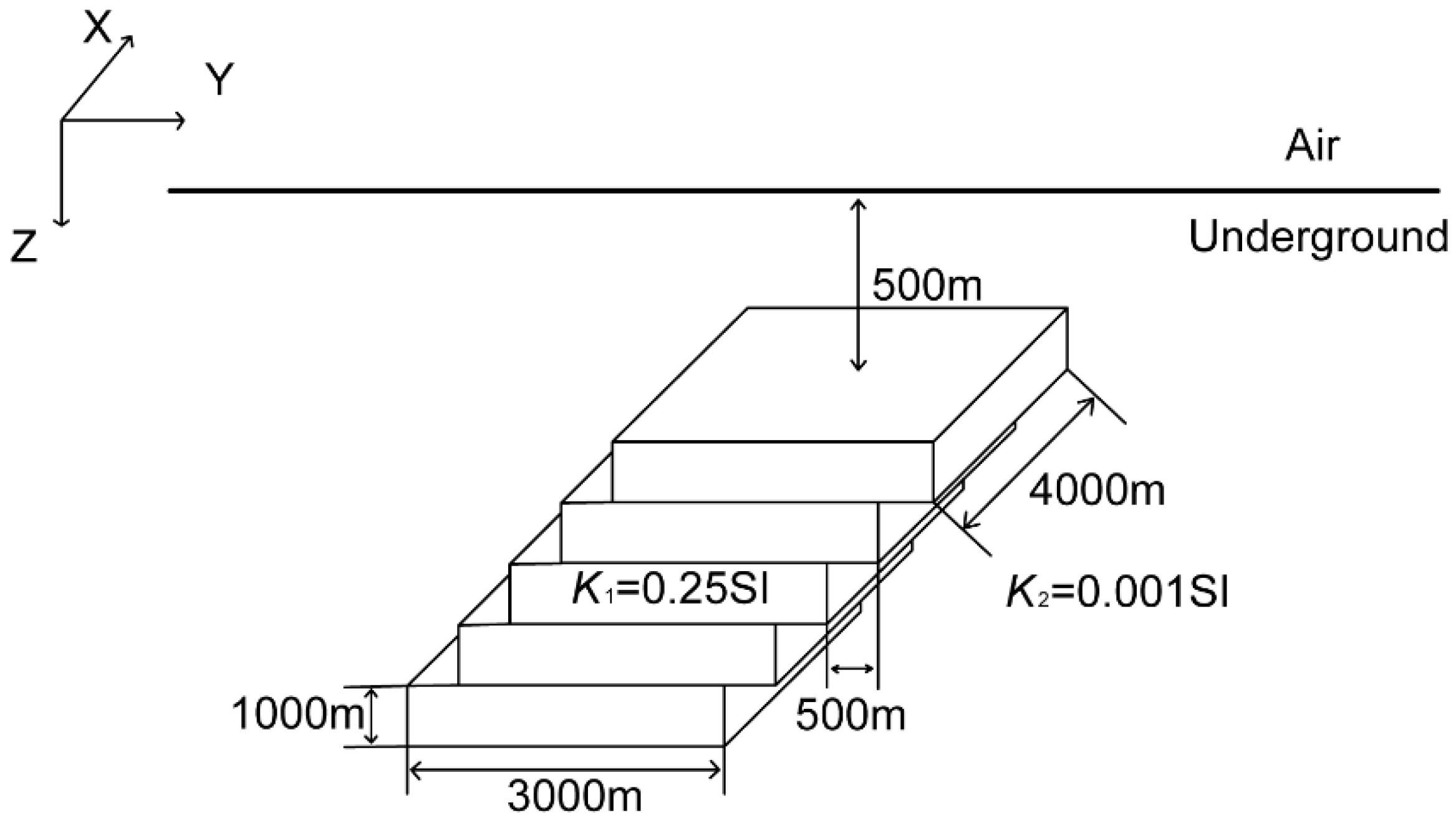
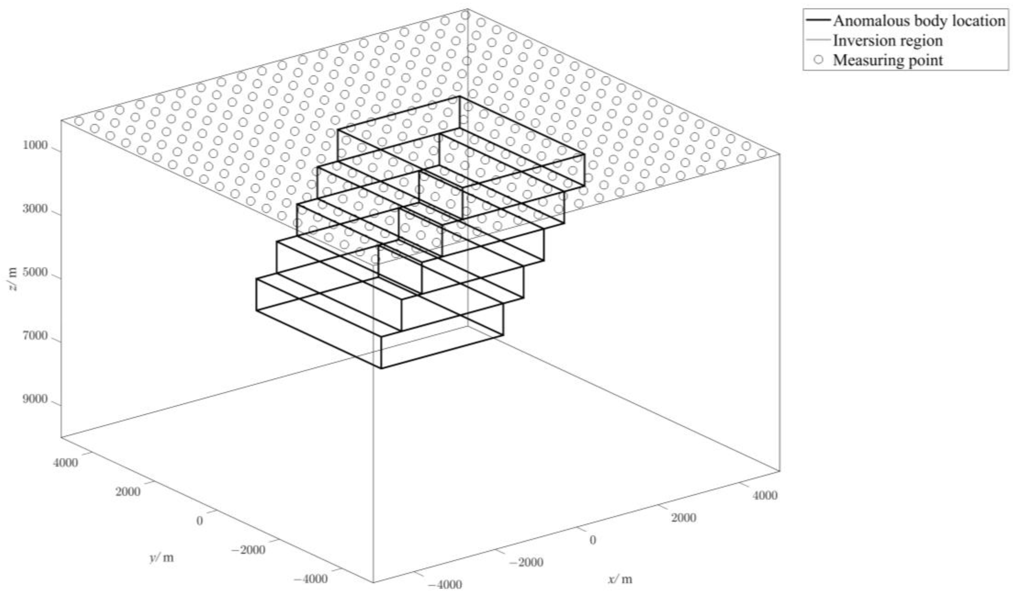
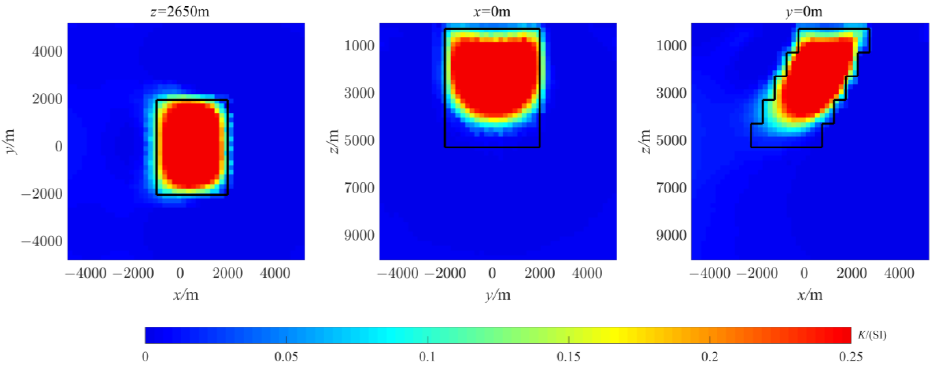
3.2. Examples of Oblique Prismatic Synthesis

As shown in Figure 7, there is a slanted prism composed of multiple single prisms in the ground, and they are buried 500 m below the surface of the earth. The inversion area is set to $10 \mathrm{k}\mathrm{m}\times 10 \mathrm{k}\mathrm{m}\times 10 \mathrm{k}\mathrm{m}$, and it is divided into 9261 cube units. The magnetic susceptibility of the anomalous body is 0.25 SI, the magnetic susceptibility of the surrounding rock is 0.001 SI, and the geomagnetic field intensity is 5000 nT. The inclination and declination of the geomagnetic field are 90° and 0°, and the inclination and declination are 90° and 0°, respectively. The measurement points are evenly arranged on the ground surface directly above the abnormal body. A total of 400 (20 × 20) measurement points are arranged, and the measurement points are represented by black circles, as shown in Figure 8. The grid distribution of the abnormal body is the same as that of the single abnormal body. Thus, according to Equation (12), $∆\mathrm{V}$ is $12.5$ × ${10}^8$, and the constant $\mathsf{\delta }$ is also 0.00179. To make the inversion closer to the actual situation, a 5% Gaussian random error is added to the synthetic data to synthesize observation data d, and the magnetic susceptibility value equal to the average magnetic susceptibility of the surrounding rock is selected as the initial inversion model.

The data fitting difference (RMS) of the inversion is shown in Figure 9. The three-dimensional limited-memory BFGS (L-BFGS) inversion based on the multiplicative objective function is iterated a total of 11 times, and the initial value of RMS converges from 6.71 to 0.88. The traditional three-dimensional inversion is iterated a total of 36 times, and the initial RMS value converges from 6.71 to 0.98. The iteration stop condition is met. The RMS descent curve of the magnetic method based on the multiplicative objective function is smooth, which proves that the magnetic method based on the multiplicative objective function has good stability and convergence.

The horizontal slice diagram and vertical slice diagram of the oblique prism obtained by means of magnetic three-dimensional limited-memory BFGS inversion based on the multiplicative objective function are shown in Figure 10. The horizontal slice diagram and vertical slice diagram of the oblique prism inversion results obtained by means of the traditional magnetic method for three-dimensional inversion are shown in Figure 11. The black boxes in both figures represent the locations of anomalous bodies. It can be seen from the figure that the positioning of the abnormal body with high magnetic permeability in the three-dimensional limited-memory BFGS inversion results based on the multiplicative objective function is more accurate, and the shape of the inversion results is closer to the real abnormal body. The true value of the abnormal body is close to the true magnetic susceptibility of the inversion model of 0.25 SI, which proves that the three-dimensional limited-memory BFGS inversion method based on the multiplicative objective function can invert the abnormal body accurately. For the skin effect, this is related to the difference in the longitudinal resolution of the magnetic method itself. Although the three-dimensional inversion results of the traditional magnetic method show a good shape recovery with regard to the abnormal body, the true value of the anomalous body is also restored to 0.25 SI, but its inversion efficiency is low. As shown in

Table 2. Comparison of the inversion efficiency of the oblique prism.

Single Prism	Iterations Number/Times	Inversion Time/Seconds	Final RMS
Limited-memory BFGS three-dimensional inversion	11	26.9	0.88
Traditional magnetic three-dimensional inversion	36	1600.6	0.98

, compared with the traditional magnetic three-dimensional inversion, the RMS of the magnetic three-dimensional finite memory pseudo-Newton inversion based on the multiplicative objective function drops below 1, and both have better inversion results. However, the magnetic three-dimensional finite memory pseudo-Newton inversion based on the multiplicative objective function takes only approximately 26 s, while the logarithmic obstacle method takes more than 1600 s. The three-dimensional finite memory quasi-Newtonian inversion with a magnetic method based on a multiplicative objective function provides a great improvement in inversion efficiency.

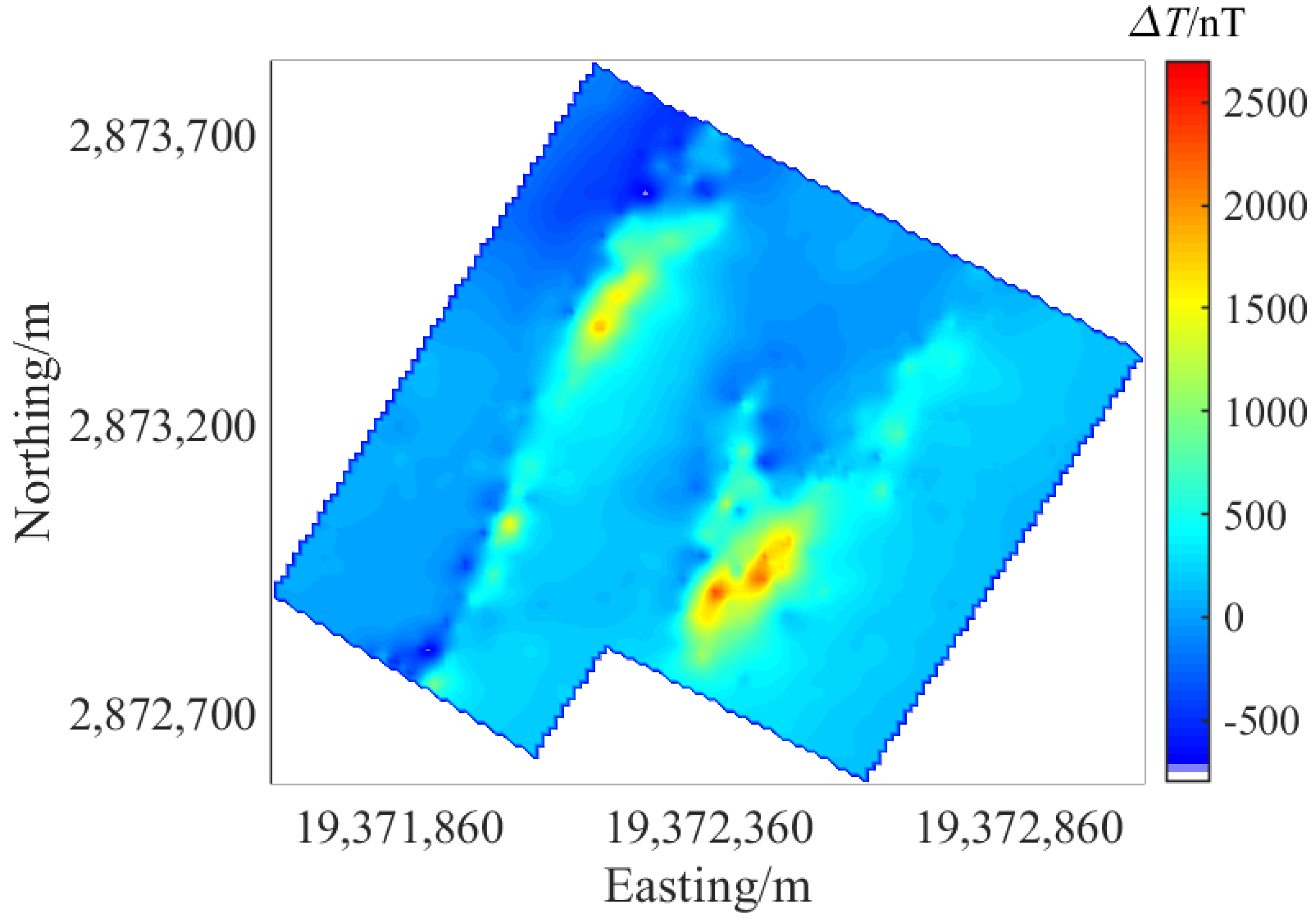
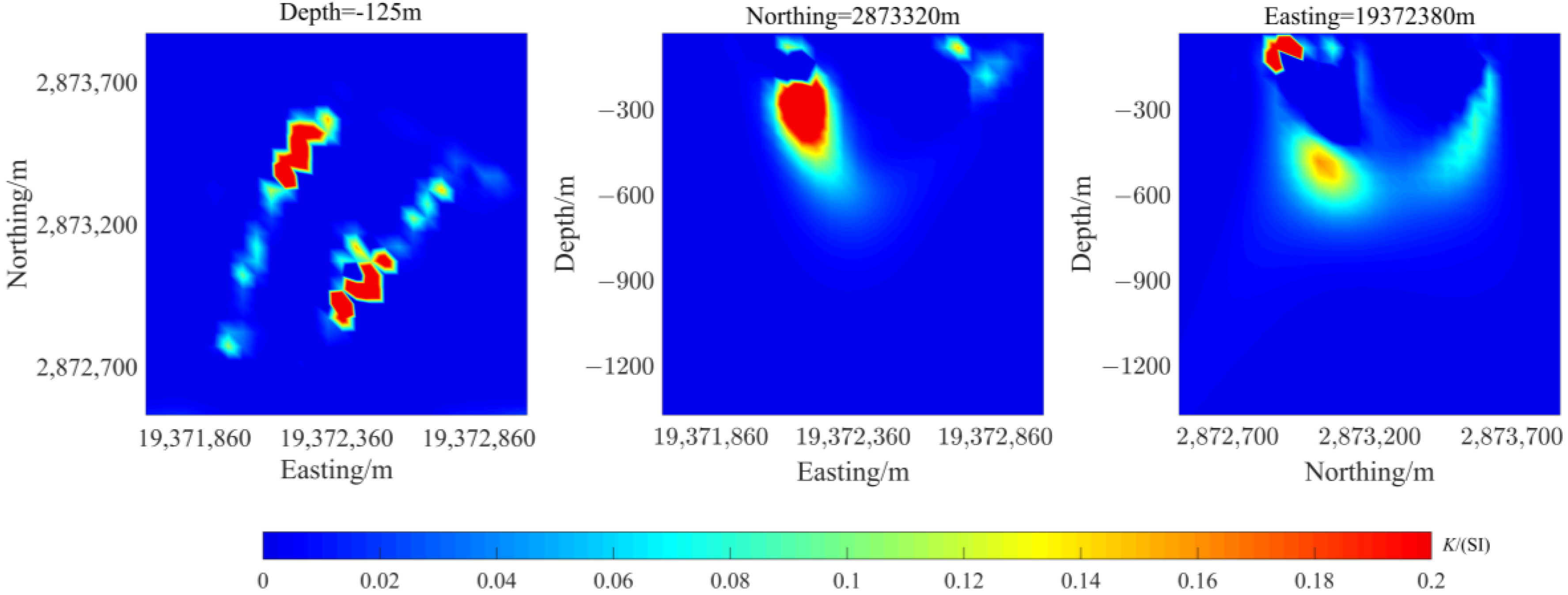
4. Measured Data Test

To further verify the feasibility and effectiveness of the three-dimensional L-BFGS inversion method based on the multiplicative objective function, this method is used to carry out an experimental calculation of the measured data.

Figure 12 shows the measured magnetic anomaly data of the Tongdao copper–nickel deposit in Hunan Province, China. The map uses the Chinese geodetic coordinate system [20]. N-type faults have developed in this area, and the copper–nickel sulphide filled by cracks is enriched in the magnetite and pyrrhotite enrichment area. Therefore, inversion can be performed to predict the spatial scope of copper–nickel deposits by locating the locations of ultrabasic rocks containing magnetite and pyrrhotite [21]. The measured data size is 141 × 125, and the grid spacing is 10 m. The magnetic field strength in this area is 47,290 nT, and the geomagnetic inclination and geomagnetic declination are 39.0° and −2.5°, respectively.

In the three-dimensional L-BFGS inversion using the magnetic method based on the multiplicative objective function, the underground subdivision is divided into $30\times 30\times 30$ cube units, and the size of the grid units is a cube with a side length of 50 m.

The data fitting difference (RMS) of the inversion is shown in Figure 13. The magnetic three-dimensional limited-memory BFGS inversion based on the multiplicative objective function is iterated a total of 20 times, and the initial RMS value converges from 6.5 to 0.98. The traditional magnetic three-dimensional inversion is iterated a total of 19 times, and the initial RMS value converges from 6.5 to 1.13, meeting the iterative stop condition. The RMS descent curve of the magnetic method based on the multiplicative objective function is smooth, which proves that the magnetic method based on the multiplicative objective function has good stability and convergence.

The measured inversion results of three-dimensional limited-memory BFGS inversion using the magnetic method based on the multiplicative objective function are shown in Figure 14, and the measured results of traditional three-dimensional inversion using the magnetic method are shown in Figure 15. The measured inversion horizontal section results of the three-dimensional limited-memory BFGS inversion based on the multiplicative objective function show that there are two obvious north-eastward faults, and the spatial distribution of underground faults can be clearly seen according to the vertical sections in both directions. The traditional magnetic three-dimensional inversion also has good results. As seen from Figure 15, the inversion results can basically distinguish two faults. In terms of the computational efficiency, as can be seen from

Table 3. Comparison of the inversion efficiency of the measured data.

Single Prism	Iterations Number/Times	Inversion Time/Seconds	Final RMS
Limited-memory BFGS three-dimensional inversion	20	35	0.98
Traditional magnetic three-dimensional inversion	19	2600	1.13

, the measurement of the three-dimensional limited-memory BFGS inversion using the magnetic method based on the multiplicative objective function takes approximately 35 s. However, the traditional three-dimensional inversion using the magnetic method takes approximately 2600 s. Compared with traditional three-dimensional inversion using the magnetic method based on a multiplicative objective function, three-dimensional limited-memory BFGS inversion using the magnetic method has higher inversion efficiency.

5. Conclusions

In this paper, based on the limited-memory BFGS (L-BFGS) method, three-dimensional magnetic inversion based on a multiplicative objective function is achieved. Through the inversion calculation of the synthetic data of the theoretical model and the measured data, the following conclusions are obtained:

(1)

The initial inversion model was developed, the maximum number of inversion iterations and the minimum fitting difference were set, the model item was calculated, the constant value was added, and depth weighting on the initial model was carried out;

(2)

Inversion based on a multiplicative objective function can be used to more easily determine the weight factor of the regularization constraint term in the inversion objective function, which has obvious advantages compared with traditional inversion based on an additive objective function.

The research results of this paper show the feasibility and effectiveness of the three-dimensional limited-memory BFGS inversion method based on the product objective function, and provide a more effective reference method for the complex problem of selecting the weight factors of the constraint terms of the objective function in geophysical fields.

References

1. Maksimov, M.A.; Surodina, I.V. Three-dimensional forward and inverse modelling of multi-height magnetic data using the relief maps. Russ. J. Geophys. Technol. 2020, 2, 4–11. [Google Scholar] [CrossRef]
2. Liu, S.; Fedi, M.; Hu, X. 3D inversion of magnetic data in the simultaneous presence of significant remanent magnetization and self-demagnetization: Example from Daye iron-ore deposit, Hubei province, China. Geophys. J. Int. 2018, 215, 614–634. [Google Scholar] [CrossRef]
3. Geng, M.; Ali, M.Y.; Fairhead, J.D.; Pilia, S.; Bouzidi, Y.; Barkat, B. Crustal structure of the United Arab Emirates and northern Oman Mountains from constrained 3D inversion of gravity and magnetic data: The Moho and basement surfaces. J. Asian Earth Sci. 2022, 231, 1–19. [Google Scholar] [CrossRef]
4. Yan, J.; Lü, Q.; Qi, G.; Fu, G.; Zhang, K.; Lan, X.; Guo, X.; Wei, J.; Luo, F.; Wang, H.; et al. A 3D Geological Model Constrained by Gravity and Magnetic Inversion and its Exploration Implications for the World-class Zhuxi Tungsten Deposit, South China. Acta Geol. Sin. Engl. Ed. 2020, 94, 1940–1959. [Google Scholar]
5. Dandan, J.; Zhaofa, Z.; Shuai, Z.; Guan, Y.; Lin, T.; Lu, P. Three-Dimensional Magnetic Inversion Based on an Adaptive Quadtree Data Compression. Appl. Sci. 2020, 10, 7636. [Google Scholar]
6. Emad, G.; Jan, D. Joint gravity and magnetic inversion with trans-dimensional alpha shapes and autoregressive noise models. Inverse Probl. 2022, 38, 890–892. [Google Scholar]
7. Wolde, M.T. Applications of Magnetic Method in Mapping Subsurface Structures in the Ziway Langano Corridor Central Main Ethiopian Rift. J. Geol. Geophys. 2021, 10, 991. [Google Scholar]
8. Li, Y.; Oldenburg, D.W. 3-D inversion of magnetic data. Geophysics 1996, 61, 394–408. [Google Scholar]
9. Li, Y.; Oldenburg, D.W. Fast inversion of large-scale magnetic data using wavelet transforms and a logarithmic barrier method. Geophys. J. Int. 2003, 152, 251–265. [Google Scholar] [CrossRef]
10. Yan, Z.; Tan, H.; Peng, M.; Kong, W.; Wu, P. Three-dimensional joint inversion of gravity, magnetic and magnetotelluric data based on cross-gradient theory. Chin. J. Geophys. 2020, 63, 736–752. [Google Scholar]
11. Alpak, F.; Gao, G.; Florez, H.; Shi, S.; Vink, J.; Blom, C.; Saaf, F.; Wells, T. A machine-learning-accelerated distributed LBFGS method for field development optimization: Algorithm, validation, and applications. Comput. Geosci. 2023, 27, 425–450. [Google Scholar]
12. Wang, K.; Tan, H.; Lin, C.; Yuan, J.; Wang, C.; Tang, J. Three-dimensional tensor controlled-source audio-frequency magnetotelluric inversion using LBFGS. Explor. Geophys. 2017, 49, 268–284. [Google Scholar] [CrossRef]
13. Abubakar, A.; Van den Berg, P.M.; Mallorqui, J.J. Imaging of biomedical data using a multiplicative regularized contrast source inversion method. IEEE Trans. Microw. Theory Tech. 2002, 50, 1761–1771. [Google Scholar] [CrossRef]
14. Li, M.; Abubakar, A.; Van den Berg, P.M. Application of the multiplicative regularized contrast source inversion method on 3D experimental Fresnel data. Inverse Probl. 2009, 25, 24006–24028. [Google Scholar] [CrossRef]
15. van den Berg, P.M.; van Broekhoven, A.L.; Abubakar, A. Extended contrast source inversion. Inverse Probl. 1999, 15, 1325–1344. [Google Scholar] [CrossRef]
16. Alpak, F.O.; Habashy, T.; Abubakar, A.; Torres-Verdin, C.; Sepehrnoori, K. A multiplicative regularized gauss-newton algorithm and its application to the joint inversion of induction logging and near-borehole pressure measurements. Prog. Electromagn. Res. B 2011, 29, 105–138. [Google Scholar] [CrossRef]
17. Xie, H.; Tan, H.; Ma, F. Three-dimensional resistivity inversion based on product type objective function. Geoscience 2023, 37, 67–73. [Google Scholar]
18. Guan, Z. Geomagnetic Field and Magnetic Exploration; Geological Publishing House: Beijing, China, 2005; Volume 7, pp. 119–121. [Google Scholar]
19. Abubakar, A.; Li, M.; Pan, G.; Liu, J.; Habashy, T.M. Joint MT and CSEM data inversion using a multiplicative cost function approach. Geophysics 2011, 76, 203–214. [Google Scholar] [CrossRef]
20. Chen, J. Modern Geodetic datum of China: China Geodetic Coordinate System 2000(CGCS 2000) and its framework. Acta Geod. Et Cartogr. Sin. 2008, 3, 269–271. [Google Scholar]
21. Li, Z.; Yao, C.; Zheng, Y.; Wang, J.; Zhang, Y. 3D magnetic sparse inversion using an interior-point method. Geophysics 2018, 83, 15–32. [Google Scholar] [CrossRef]
Figure 1. Cube unit diagram.
Applsci 13 11198 g001
Figure 2. Single prism anomaly.
Applsci 13 11198 g002
Figure 3. Schematic diagram of the observation system.
Applsci 13 11198 g003
Figure 4. Fitting difference curve of the single prism model inversion data.
Applsci 13 11198 g004
Figure 5. Inversion results of three-dimensional L-BFGS inversion of a single prism model based on a multiplicative objective function using the magnetic method.
Applsci 13 11198 g005
Figure 6. Inversion results of the traditional three-dimensional magnetic inversion single prism.
Applsci 13 11198 g006
Figure 7. Oblique prism anomaly.
Applsci 13 11198 g007
Figure 8. Schematic diagram of the observation system.
Applsci 13 11198 g008
Figure 9. Fitting difference curve of the oblique prism model inversion data.
Applsci 13 11198 g009
Figure 10. Inversion results of three-dimensional L-BFGS inversion of the oblique prism model based on the multiplicative objective function.
Applsci 13 11198 g010
Figure 11. Inversion results of the traditional magnetic three-dimensional inversion of the oblique prism model.
Applsci 13 11198 g011
Figure 12. Magnetic anomaly.
Applsci 13 11198 g012
Figure 13. Fitting difference curve of the measured data inversion.
Applsci 13 11198 g013
Figure 14. Inversion results of the three-dimensional L-BFGS inversion of measured data based on the multiplicative objective function.
Applsci 13 11198 g014
Figure 15. Inversion results of the traditional magnetic three-dimensional inversion of measured data.
Applsci 13 11198 g015