Coverage Optimization of WSNs Based on Enhanced Multi-Objective Salp Swarm Algorithm

Abstract

In complex two-dimensional monitoring environments, how to enhance network efficiency and network lifespan while utilizing limited energy resources, and ensuring that wireless sensor networks achieve the required partial coverage of the monitoring area, are the challenges of optimizing coverage in wireless sensor networks.With the premise of ensuring connectivity in the target network area, an enhanced multi-objective salp swarm algorithm based on non-dominated sorting (EMSSA) is proposed in this paper, by jointly optimizing network coverage, node utilization, and network energy balance objectives. Firstly, the logistic chaotic mapping is used to maintain the diversity of the initial salp swarm population. Secondly, to balance global and local search capabilities, a new dynamic convergence factor is introduced. Finally, to escape local optima more effectively, a follower updating strategy is implemented to reduce the blind following of followers while retaining superior individual information. The effectiveness of the strategy is validated through comparative experiments on ZDT and DTLZ test functions, and the proposed algorithm is applied to coverage optimization in WSNs in complex environments. The results demonstrate that the algorithm can adjust coverage thresholds according to different application requirements, providing various effective coverage optimization configurations. With the same preset requirements for partial coverage achieved, both network efficiency and lifespan have been significantly improved.

1. Introduction

Wireless sensor networks (WSNs) is a multi-hop self-organizing network composed of a large number of sensor nodes used for monitoring physical events [1]. Due to their outstanding performance advantages, they play a crucial role in various fields such as environmental monitoring, healthcare, agriculture, and urban traffic [2,3,4,5], contributing significantly to the development and application of Internet of Things (IoT) technology.

Coverage optimization is an important research direction in the field of WSNs. The distribution of nodes within the monitoring area, among other factors, determines the sensing coverage capability of WSNs. Additionally, the sensing and monitoring capabilities within the monitoring area determine whether the WSNs can provide effective monitoring services. In practical applications, when deploying wireless sensor nodes in complex environments such as forests or oceans that are difficult for humans to access, the typical approach is to deploy them in a random manner, which can lead to issues such as decreased network performance and resource wastage. Deploying mobile nodes is a commonly used coverage optimization method to improve network coverage, but this approach significantly increases deployment costs. Therefore, designing appropriate node deployment strategies is crucial for effectively enhancing the monitoring performance and data transmission quality of WSNs while keeping energy consumption at an acceptable level. This plays a pivotal role in the future development of the entire WSNs application landscape.

The application of swarm intelligence algorithms and their improved algorithms in the field of WSNs coverage optimization is quite common. Scholars continuously analyze and research swarm intelligence algorithms and have proposed various bio-inspired algorithms. These include the Particle Swarm Optimization (PSO) [6] algorithm, which simulates the foraging behavior of bird flocks; the Flower Pollination Algorithm (FPA) [7], which mimics the pollination process of flowering plants in nature; the Fruit Fly Optimization Algorithm (FOA) [8], which is based on the foraging behavior of fruit flies; the Firefly Optimization Algorithm (FA) [9], which imitates fireflies’ aggregation through bioluminescence; the Grey Wolf Algorithm (GWO) [10], inspired by the hierarchical hunting behavior of wolf packs; the Whale Optimization Algorithm (WOA) [11], derived from the behavior of whales capturing food; The salp swarm algorithm, inspired by the aggregative behavior of salp swarm [12]; and various related improved or hybrid algorithms. However, existing research on coverage optimization for network coverage can only ensure a more reasonable distribution of nodes, with relatively limited improvements in network performance. Comprehensive coverage optimization studies for WSNs, considering objectives such as network coverage, connectivity, and node energy consumption, are more practically valuable. Typically, multiple-objective optimization algorithms are used to comprehensively optimize these multiple objectives.

Most existing research on WSNs coverage optimization has overlooked the variability in coverage requirements within the monitoring target area [13,14,15,16,17]. It generally assumes that the monitoring area has uniform coverage requirements. However, in real-world scenarios where different levels of monitoring coverage are needed, this assumption may not hold. This can lead to partial coverage issues when users specify their required coverage thresholds based on their actual business needs. Nonetheless, in many cases, partial coverage is sufficient to meet business requirements and can be achieved with fewer active nodes, thus extending the network’s lifespan.

To address the challenge of balancing network coverage, node utilization, and node energy consumption in WSNs coverage optimization, this paper introduces an enhanced multi-objective salp swarm algorithm (EMSSA). The MSSA algorithm [12] for solving multi-objective problems has some drawbacks, such as premature convergence and susceptibility to getting stuck in local optima. Therefore, further improvements are needed for the MSSA algorithm. The enhanced algorithm (EMSSA) is then applied to the study of sensor node deployment in complex environments. The primary contributions of this research are summarized as follows.

• Considering network coverage, node utilization, and network energy balance, a multi-objective optimization deployment model is proposed for WSNs coverage optimization.
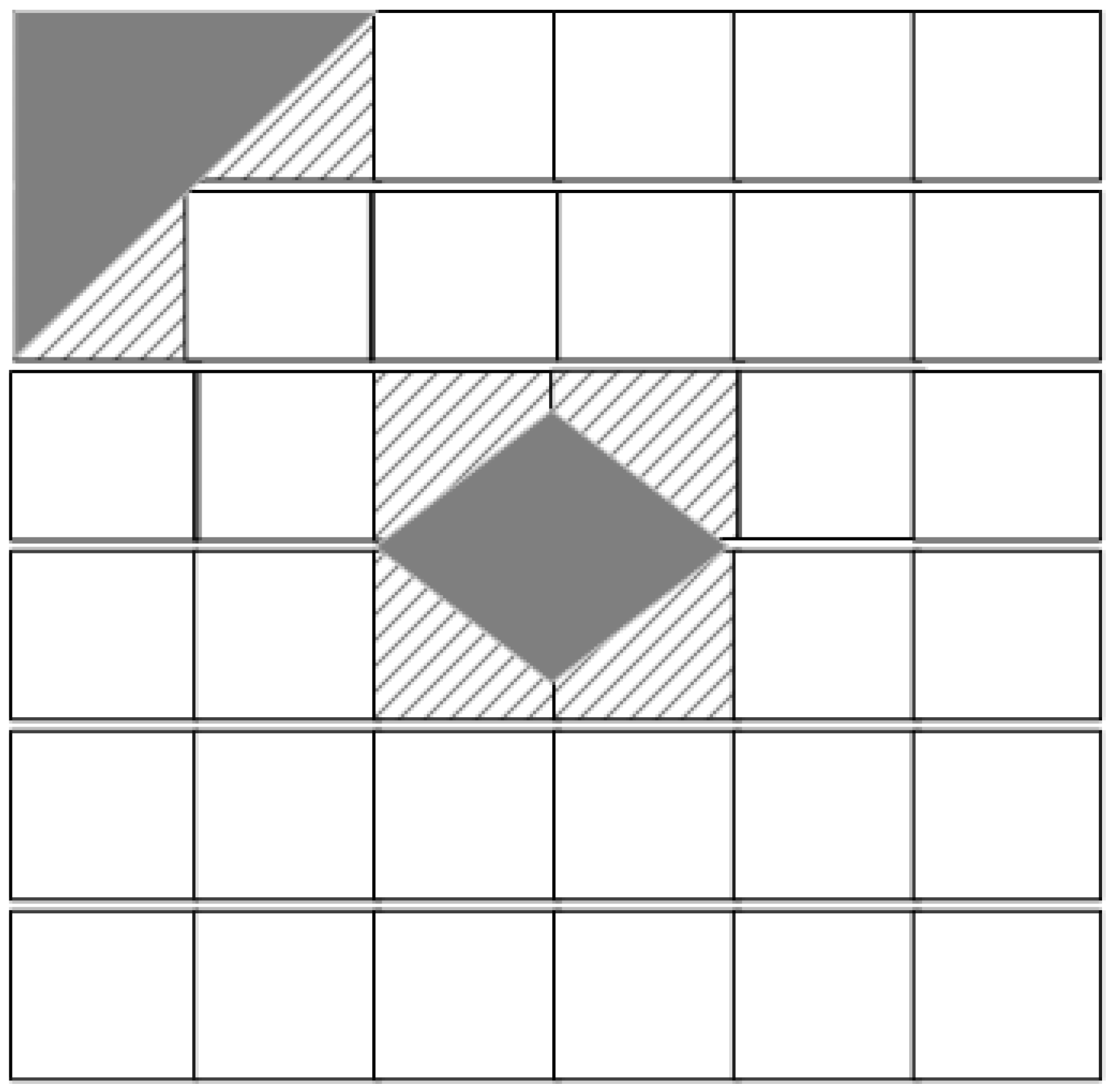
• To deploy sensor nodes in effective positions, we propose a grid-based approach for monitoring areas with obstacles.
• Based on the multi-objective optimization model proposed in this paper, we have designed an enhanced multi-objective salp swarm algorithm (EMSSA) based on multiple strategies.
• Finally, we applied the proposed algorithm in a complex environment, providing different effective coverage optimization configurations by adjusting coverage thresholds for node deployment.

The remaining of the paper is organized as follows. Recent relevant works in the literature are discussed in Section 2. In Section 3, we provide a detailed description of our proposed multi-objective optimization deployment model. The algorithm is explained in Section 4. Subsequently, we discuss our simulation experiments and their results in Section 5. while the Section 6 concludes the paper and provides future research directions.

2. Related Works

In recent years, researchers have conducted extensive work on coverage optimization in WSNs, achieving significant advancements.

Swarm intelligence optimization algorithms possess several advantages, such as strong search capabilities and inherent randomness. Utilizing intelligent optimization algorithms in coverage optimization, based on these algorithms, has become increasingly common across various domains, including the optimization deployment of wireless sensor nodes. In order to enhance the Quality of Service (QoS) in WSNs and extend network lifespan, Ying et al. [13] improved the classical multi-objective Ant Lion Optimization (MOALO) algorithm and proposed an enhanced MOALO algorithm based on fast non-dominated sorting (NSIMOALO). Yao et al. [14], addressing the issue of nodes deviating from the optimal deployment positions in complex monitoring areas like battlefields and disaster zones, resulting in coverage holes, introduced a WSNs coverage enhancement strategy based on Virtual Force-directed Ant Lion Optimization (VF-IALO). Experimental results demonstrated the effectiveness of the proposed improved algorithms. Yao et al. [15], addressing the optimization problem of maximizing coverage. Inspired by the predation behavior of Army Ants, this paper introduces a novel swarm intelligence (SI) technique called the Army Ant Search Optimizer (AASO) to tackle the problem of maximizing coverage. Simulation results demonstrate that WMSNs (Wireless Multimedia Sensor Networks) enhanced with AASO exhibit superior coverage performance. To balance coverage and average node movement distance, Wang et al. [16] combined Virtual Force Algorithm (VFA) with Grey Wolf Optimizer (GWO) and proposed the VFA-based Lévy Flight GWO for coverage optimization in WSNs. Simulation experiments demonstrated the algorithm’s strong applicability as the number of nodes and monitoring area size varied. Addressing the issue of heterogeneous node deployment optimization in WSNs with obstacles in the monitoring area, Wang et al. [17] introduced two new Flower Pollination Algorithms (FPA) for network deployment. Simulation experiments indicated that both improved algorithms could provide better solutions for WSNs deployment.

Bouzid et al. [18] proposed a novel approach for optimizing node placement, referred to as MOONGA (Multi-Objective Optimization for WSNs using Genetic Algorithms). It can generate optimal deployments based on topology, environment, specifications of different applications, as well as the preferences of network designers and users. Khalaf et al. [19] introduced a Bee algorithm to maximize network coverage area, significantly expanding the area covered while reducing coverage gaps. However, the algorithm exhibits poor convergence. Zain Eldin et al. [20], in response to the issues of network coverage gaps and high deployment costs, proposed an improved Genetic Algorithm-based dynamic deployment technique that achieves maximum target area coverage with the fewest nodes. Addressing the problems of high coverage costs and node failures leading to inadequate monitoring, Al-Fuhaidi et al. [21] presented an efficient deployment model based on a probabilistic sensing model and the Harmony Search algorithm. This model balances coverage performance and deployment costs. Elhoseny et al. [22] introduced a novel model combining Genetic Algorithms to meet WSNs coverage requirements. This model aims to monitor targets for as long as possible with limited energy, but it has a relatively high algorithmic complexity. Syed et al. [23] proposed a strategy based on weighted distance location updates, known as the Weighted Salp Swarm Algorithm (WSSA). Simulation results have confirmed the improved performance and convergence speed of WSSA. Furthermore, the WSSA method has been applied to a probabilistic sensor model to maximize coverage range and to a wireless energy model to minimize energy consumption.

WSNs coverage optimization can be categorized into two types based on the number of optimization objectives: single-objective optimization and multi-objective optimization. Multi-objective optimization problems can further be classified into two major categories. One category is linear weighting, where the idea is to integrate the solutions to multiple objectives into a single objective for optimization. For example, to achieve the goal of minimizing energy consumption and sensor node overlap area, Céspedes-Mota et al. [24] used a Multi-Objective Differential Evolution Algorithm (MODEA) to optimize the distribution of sensor nodes in regular and irregular regions. Different weights were assigned to each objective, transforming the multi-objective optimization into a single optimization problem. The other category is Pareto-based, where direct optimization of multiple objectives is performed. Benatia et al. [25], for instance, proposed a multi-objective deployment strategy that considers sensor node positions and network cost. They then used a multi-objective evolutionary algorithm to search for global optimal solutions. Harizan et al. [26] proposed the use of the multi-objective evolutionary algorithm NSGA-II to address the multi-objective problem of coverage and connectivity. They linearly programmed the multi-objective problem and introduced chromosome crossover and mutation methods to enhance the algorithm’s performance. In order to increase coverage while reducing node energy consumption, Xu et al. [27] utilized the MOEA/D-I and MOEA/D-II algorithms to jointly optimize network coverage, energy consumption rate, and energy balance rate. Wang et al. [28] aimed to optimize network coverage, energy consumption rate, and energy balance rate, and they integrated these three optimization objectives into a single objective using linear weighting. They then employed an improved Whale Algorithm to optimize this single objective function.

3. Multi-Objective Optimization Deployment Model

3.1. Perception Model

The Boolean model overlooks the influence of real-world factors on wireless sensor nodes, and a simplified model may have some impact on the research. In actual monitoring environments, the sensing capability of sensor nodes can be disrupted by obstacles within the monitoring range, leading to a gradual decrease in the detection probability for monitoring targets beyond a certain range. In a probabilistic sensing model, the perception probability of sensor nodes for the monitoring area is set to be distance-dependent and follows an exponential relationship.

In WSNs, assuming a set of wireless sensor nodes $s=\{s_1,s_2,\cdots ,s_i,\cdots ,s_n\}$, a set of grid points $P=\{P_1,P_2,\cdots ,P_j,\cdots ,P_n\}$, $(x_i$, $y_i)$ and $(x_j,y_j)$ corresponding to the 2D spatial coordinates in their respective sets of $s_i$ and $P_j$, the Euclidean distance between two nodes is given by

$$d(s_i,P_j)=\sqrt{\begin{array}{ccc}{(x_i-x_j)}^2& +& {(y_i-y_j)}^2\end{array}}$$

(1)

According to the definition of the probability perception model, the probability of monitoring point $P_j$ being sensed by node $s_i$ is given by

$$P_{\mathrm{cov}}(s_i,P_j)=\left\{\begin{array}{c}1\\ e^{-\lambda {\alpha }^{\beta }}\\ 0\end{array}\begin{array}{c}d(s_i,P_j)\le R-r\\ R-r<d(s_i,P_j)<\\ d(s_i,P_j)\ge R+r\end{array}\right.R+r$$

(2)

where R represents the sensing radius of the sensor node, and r is the reliability monitoring parameter of the sensor node, with the typical value being $0<r<R$. The variables $\alpha$ and $\beta$ are the attenuation coefficients of the sensing capability of the sensor node, and  $\lambda$ is an input parameter derived by

$$\lambda =d(s_i,P_j)-(R-r)$$

(3)

3.2. Determining the Multi-Objective Deployment Model

3.2.1. Coverage Model

For the specific scenario of deploying nodes in complex environments with obstacles in this paper, we can make the following assumptions:

• Sensor nodes are of the same type and have identical physical characteristics, with a communication radius set to twice the sensing radius.
• Sensor nodes can determine their own positions and can move to specified locations based on the algorithm [29,30].
• The positions of obstacles within the monitoring area are known in advance.

Node coverage rate is one of the important metrics for assessing the overall monitoring quality of WSNs. In this paper, we first gridify the monitoring area, considering the center of each grid as a target monitoring point. Subsequently, the number of target monitoring points covered by the grid representation of the monitoring area is used as the coverage area of the sensor nodes in the monitoring area.

The probability of node $s_i$ perceiving monitoring point $P_j$ is represented in Formula (2). $s_{all}$ represents all the nodes in the monitoring area, so the joint perception probability of all sensor nodes for point $P_j$ is defined as

$$C_p(s_{all},P_j)=1-\prod _{s_i\subseteq s}(1-P_{\mathrm{cov}}(s_i,P_j)).$$

(4)

The coverage rate of sensor nodes in an environment with obstacles is represented by

$$Cov(X_i)=\frac{{\displaystyle \sum _{j=1}^G}{C}_P(s_{all},P_j)}{G-K}$$

(5)

where G represents the total number of target monitoring points after the gridding of the monitoring area, and K indicates the number of vertices in the grid cells occupied by obstacles.

3.2.2. Node Utilization Model

Due to the limited energy and processing capacity of nodes, the number of nodes is also constrained. In practical applications, to maintain the normal operation of the entire network within a specified working time, it is often necessary to minimize the number of active nodes as much as possible and extend the lifespan of sensor nodes. Node utilization rate is defined as

$$U_{\eta }=\frac{\sum e_i}{N}$$

(6)

where $e_i$ represents the number of active and effective nodes, and N represents the total number of sensor nodes. A smaller value of $U_{\eta }$ indicates lower node utilization, indicating that there are more sleeping nodes, thus extending the network’s lifespan. Conversely, with fewer sleeping nodes, the network’s operational time is shorter.

3.2.3. Energy Consumption Model

Sensor nodes are typically powered by batteries and cannot replenish energy after deployment in the monitoring area. Therefore, energy efficiency is an important evaluation metric in the field of coverage technology for WSNs.

Definition 1.

Energy of Zone $E_k$

$E_k$ is obtained by dividing the monitoring area into K equal grids, where k within the range $[1,M]$. The energy of the k-th grid is defined as the ratio of the cumulative remaining energy of all nodes within this grid to the total number of nodes in this grid, given by

$$E_k=\frac{{\sum }_{i=1}^{m_k}{E}_{ki}}{m_k}$$

(7)

where $m_k$ represents the number of nodes in the k-th grid, and $E_{ki}$ denotes the remaining energy of node i in the k-th grid.

Definition 2.

Energy of Zone $E_a$

$E_a$ is defined as the difference between the maximum and minimum values of the grid energy divided by the maximum grid energy, representing the current energy balance level of the network in

$$E_a=\frac{max(E_k)-min(E_k)}{max(E_k)}$$

(8)

where $E_a$ reflects the overall balance of energy consumption in the network, where a larger value indicates a more uneven energy consumption. Therefore, a smaller $E_a$ corresponds to better network performance.

3.2.4. Description of Multi-Objective Problem

The ultimate optimization goal of this paper is to ensure coverage that meets the requirements of the monitoring area while using as few sensor nodes as possible and extending the overall network lifespan. The lower the energy consumption, the longer the network’s lifespan. The multi-objective sensor network deployment problem described in this paper can be characterized as

$$\left\{\begin{array}{c}{f}_1(O)=Max(Cov(O))\\ f_2(O)=Min(U_{\eta }(O))\\ f_1(O)=Min(E_a(O))\\ \begin{array}{cc}s.t& s=\left\{s_1,s_2,\cdots ,s_i,\cdots s_N\right\}\in H\end{array}\end{array}\right.$$

(9)

where the constraint $A(s_i)\in H$ that each node’s position ($s_i$) must be within the monitoring area (H). Here, O represents a matrix containing the coordinates, remaining energy, sensing radius, and communication radius of a set of sensor nodes.

3.3. Obstacle Handling Description

3.3.1. Approximate Grid-Based Obstacle Handling

The gridding of obstacles within the monitoring area is subject to two specific assumptions:

• The locations of obstacles can be obtained in advance.
• The grid size should be significantly smaller than the size of the obstacles, as the grid size directly affects the accuracy of obstacle detection and coverage range estimation.

The method of gridding obstacles is illustrated in Figure 1. When an obstacle covers an entire grid or when the boundaries of an obstacle fall within a grid, that grid is marked as an obstacle grid.

3.3.2. Obstacle Handling

In this paper, diamond and triangular obstacles are introduced within a square monitoring area, as shown in Figure 2. When optimizing the deployment algorithm, the nodes that fall within the obstacles need to be processed as follows:

• When a node is located within a diamond-shaped obstacle (e.g., Node A): To minimize power consumption caused by excessive node movement distance, a vertical line is drawn from Node A to the nearest boundary of the diamond-shaped obstacle. The intersection point between the perpendicular line and the boundary is denoted as point A’. Node A is then repositioned at point A’ as its corrected location.
• When a node falls within a triangular obstacle (e.g., Node B): A vertical line is drawn from Node B to the slant side of the triangle. The intersection point between the perpendicular line and the slant side is denoted as point B’. Node B is then repositioned at point B’ as its corrected location.

3.4. Network Connectivity Description

WSNs are task-oriented networks that revolve around data and sense the monitoring area, with nodes transmitting data through single-hop or multi-hop wireless communication. For the sake of computation, it is assumed that $2R=R_c$. A directed graph adjacency matrix M is established, which is used to store the connectivity status between any two nodes. Connectivity is determined based on Formula (10), where $M\left[i\right]\left[j\right]=1$ indicates that node i can transmit information to node j. Subsequently, the overall network connectivity is determined using the matrix $S_v$ calculated according to Formula (11)

$$M\left[i\right]\left[j\right]=\left\{\begin{array}{cc}1& \begin{array}{cc}if& d\left(s_i,s_j\right)\le R_i^c\end{array}\\ 0& otherwise\end{array}\right.$$

(10)

$$S_v=M+M^2+M^3+\cdots M^{n-1}$$

(11)

where n is the number of sensor nodes, if all elements in the vector $S_v$ are 1, it indicates that the network is connected; otherwise, it indicates that the network is disconnected. On the basis of WSNs connectivity, the Kruskal algorithm mentioned in [31] is used to generate the Minimum spanning tree.

4. Enhanced Multi-Objective Salp Swarm Algorithm (EMSSA)

4.1. Description of the Mathematical Model for Moving Salp Chains

The Salp Swarm belongs to the family Ascidiidae and has a transparent barrel-shaped body. It establishes a chain model for solving optimization problems, dividing the salps into two groups: leaders and followers. Leaders are the salps located at the front of the food chain, while the rest are considered followers. The population is initialized as shown in

$$X_{N\times d}=rand(N,d)\times (ub-lb)+lb$$

(12)

where N is the population number and d is the dimension, $ub$ and $lb$ respectively denote the upper and lower bounds of the search space, and $rand(N,d)$ is a random array of N rows and d columns between $[0,1]$.

The position update formula for leaders is as follows

$$X_d^1=\left\{\begin{array}{c}{F}_j+c_1((u{b}_j-l{b}_j)c_2+l{b}_j)\\ F_j-c_1((u{b}_j-l{b}_j)c_2+l{b}_j)\end{array}\right.\begin{array}{c}\\ \end{array}\begin{array}{c}{c}_3\ge 0.5\\ c_3<0.5\end{array}.$$

(13)

where $X_d^1$ represents the position of the first leader in the j-th dimension, $F_j$ represents the position of the food source in the j-th dimension, $u{b}_j$ and $l{b}_j$ are the upper and lower bounds of the j-th dimension, respectively. The coefficient $c_1$ is the most important parameter in SSA, as it balances exploration and exploitation, and it is defined as follows

$$c_1=2e^{-{(4t/T)}^2}$$

(14)

where t represents the current iteration, T represents the maximum number of iterations. The parameters $c_2$ and $c_3$ are random numbers uniformly generated within the interval [0, 1].

The update of the follower’s position, as shown in

$$X_d^i=\frac{1}{2}(X_d^i+X_d^{i-1}).$$

(15)

where $i\ge 2$, and $X_d^i$ represents the position of the i-th follower in the j-th dimension.

4.2. Enhanced Multi-Objective Salp Swarm Algorithm (EMSSA)

The solution to multi-objective problems is a set of solutions known as the Pareto optimal set. The SSA algorithm can drive salps toward food sources and update them during the iteration process. However, this algorithm cannot solve multi-objective problems. In 2017, Mirjalili et al. proposed a Multi-Objective Salp Swarm Algorithm (MSSA) [12] to address multi-objective optimization problems. Although it has high convergence and coverage, it still has some shortcomings, such as susceptibility to local optima and relatively slow convergence speed. To enhance MSSA’s convergence speed, exploration and exploitation capabilities, and escape from local optima, this paper presents further improvements to the MSSA algorithm.

4.2.1. Logistics Chaotic Mapping

The initialization of the salps population is crucial for the convergence speed and optimization accuracy of MSSA. In order to increase the likelihood of obtaining good initial solution positions and accelerate the convergence of the population, this paper adopts the Logistics chaotic mapping method, which has better traversal uniformity and faster iteration speed. This method improves the coverage space of initial solutions, and the calculation is as follows

$$x_{j+1}^i=\mu x_j^i\left(1-x_j^i\right)\begin{array}{cc},& x_j^i\end{array}<0.5$$

(16)

In this paper, $\mu$ is set to 4, where $\mu \in \left[0,4\right]$ is the chaotic parameter, and a larger $\mu$ corresponds to stronger chaos. $i=1,2,\cdots ,N$ represents the population size, and $j=1,2,\cdots ,d$ represents the index of the chaotic variable.

4.2.2. Dynamic Convergence Factor

To balance the global and local search capabilities of MSSA, a new dynamic convergence factor is introduced during the leader’s position update. This dynamic convergence factor draws inspiration from PSO and introduces an inertia weight strategy. It also employs a sine function to control the variation of the inertia weight. This function allows the salp swarm to explore the optimal solution at a relatively high speed at the beginning, and then gradually stabilizes the local search with a smoother rate of change towards the end, facilitating the discovery of the best solution. The Formula (17) is modified as follows

$$c_1^{\prime }=sin(\pi +\pi \ast (\frac{t}{2T}))+\frac{w_{max}+w_{min}}{2}$$

(17)

When the inertia weight varies between 0.4 and 0.9, the algorithm exhibits relatively good optimization performance. As the iterations progress, the inertia weight is nonlinearly decreased from 0.9 to 0.4, achieving dynamic weight changes. This allows for a better balance between global exploration and local exploitation in the algorithm and, to some extent, increases the probability of escaping local optimal regions [32]. Therefore, in this paper, the value of $w_{max}$ is set to 0.9, and $w_{min}$ is set to 0.4.

The updated equation for the leader position is shown in Formula (18).

$$X_d^1=\left\{\begin{array}{c}{F}_j+c_1^{\prime }((u{b}_j-l{b}_j)c_2+l{b}_j)\\ F_j-c_1^{\prime }((u{b}_j-l{b}_j)c_2+l{b}_j)\end{array}\right.\begin{array}{c}\\ \end{array}\begin{array}{c}{c}_3\ge 0.8\\ c_3<0.8\end{array}$$

(18)

where $c_1^{\prime }$ represents the new dynamic convergence factor, with the meanings of the other parameters remaining the same as in Formula (13).

4.2.3. Follower Updating Strategy

In the original formula for follower position update, the movement of followers has a certain degree of randomness and is only related to the position of the previous individual. It lacks the ability to exchange information with other individuals, which can lead to the algorithm getting stuck in local optima. To address these shortcomings, this paper introduces a new formula for follower position update, which is expressed as follows

$$L=1-\frac{t}{T}$$

(19)

where t represents the current iteration count, T represents the maximum number of iterations, and the value of L decreases from 1 to 0 as the iteration t progresses.

$$X_d^i=\left\{\begin{array}{c}(X_d^{i-1}+L{X}_d^i)/2\\ X_d^{i-1}-sin(X_d^i)\end{array}\right.\begin{array}{c}\hfill \end{array}\begin{array}{c}f(X_d^{i-1})\le f(X_d^i)\\ f(X_d^{i-1})>f(X_d^i)\end{array}$$

(20)

where L is added in front of the individual in the better position to reduce the influence of individuals in poorer positions. Conversely, a sine mechanism is used to control the range of individual movement. This approach significantly reduces the randomness of followers, enhances information exchange between individuals, and ensures population diversity.

4.2.4. Enhanced Multi-Objective Salp Swarm Algorithm (EMSSA)

Based on the description of MSSA and the three improvement measures mentioned above, the pseudo code for EMSSA can be seen in Algorithm  1. The EMSSA algorithm first initializes the population of salps with Logistics chaotic mapping. Then, it calculates the objective values for each salp and finds the non-dominated solutions. These non-dominated solutions are updated to the repository based on the repository update mechanism. Next, a food source is selected from the non-dominated solutions in the repository with the least crowded neighborhood. The next step involves updating the position of leading/follower salps using the respective formulas. If a salp goes out of bounds during the position update process, it is brought back within the boundary. Finally, all the above steps, except for the initialization step, are repeated until the termination condition is met.

Algorithm 1: Pseudo code of the EMSSA algorithm.

5. Results and Discussion

The simulation experiments in this paper were conducted using Matlab 2021a, with identical parameters set for all simulations. To effectively demonstrate the performance of the EMSSA algorithm proposed in this paper, this section conducts convergence tests on this algorithm, the original MSSA [12] algorithm, and the multi-objective optimization genetic algorithm (NSGA-II) [33] on four different test functions. A comparative analysis is performed among the three different algorithms. Subsequently, coverage optimization is carried out using these three algorithms at various coverage thresholds to derive experimental conclusions.

5.1. Performance Analysis of the Proposed Algorithm

To validate the effectiveness of the EMSSA algorithm, four challenging multi-objective test functions were selected for benchmarking. Due to the complexity of these multi-objective test functions, a larger number of search agents (60) and a higher maximum iteration limit (1000) were employed. It is worth noting that the maximum archive size for both MSSA and EMSSA was set to 100 in

Table 1. Parameter Setting.

Algorithm	Parameters
NSGA-II	$pc=0.9,pm=1/n,\eta c=\eta m=20$
MSSA	$c_2\in \left[0,1\right],c_3\in \left[0,1\right],repository=100$
EMSSA	$c_2\in \left[0,1\right],c_3\in \left[0,1\right],repository=100$

, and the parameter settings for the test functions are shown in

Table 2. Test Function Parameter Settings.

Function	Dimension		Pareto Front
	Variables	Objectives	Number of Samples
ZDT1	30	2	1000
ZDT2	30	2	1000
ZDT3	30	2	536
DTLZ7	22	3	4700

. After running the algorithm for 30 iterations, quantitative results were calculated using the IGD measure, as shown in

Table 3. Results of the three algorithms (using IGD) on the test functions employed.

Algorithm	ZDT1
	Ave	Std.	Best	Worst
NSGA-II	$6.25\times {10}^{-3}$	$5.21\times {10}^{-3}$	$6.05\times {10}^{-4}$	$2.16\times {10}^{-2}$
MSSA	$3.15\times {10}^{-3}$	$8.99\times {10}^{-4}$	$2.19\times {10}^{-3}$	$6.28\times {10}^{-3}$
EMSSA	$1.06\times {10}^{-4}$	$9.69\times {10}^{-5}$	$5.51\times {10}^{-4}$	$7.21\times {10}^{-4}$
Algorithm	ZDT2
	Ave	Std.	Best	Worst
NSGA-II	$1.35\times {10}^{-2}$	$1.22\times {10}^{-2}$	$6.15\times {10}^{-4}$	$4.29\times {10}^{-2}$
MSSA	$3.58\times {10}^{-3}$	$1.66\times {10}^{-3}$	$2.08\times {10}^{-3}$	$9.51\times {10}^{-3}$
EMSSA	$6.01\times {10}^{-4}$	$7.81\times {10}^{-5}$	$4.58\times {10}^{-4}$	$8.46\times {10}^{-4}$
Algorithm	ZDT3
	Ave	Std.	Best	Worst
NSGA-II	$9.52\times {10}^{-3}$	$7.03\times {10}^{-3}$	$8.32\times {10}^{-4}$	$2.25\times {10}^{-2}$
MSSA	$6.67\times {10}^{-3}$	$2.78\times {10}^{-3}$	$3.92\times {10}^{-3}$	$1.75\times {10}^{-2}$
EMSSA	$1.02\times {10}^{-3}$	$1.60\times {10}^{-4}$	$7.70\times {10}^{-4}$	$1.61\times {10}^{-3}$
Algorithm	DTLZ7
	Ave	Std.	Best	Worst
NSGA-II	$2.12\times {10}^{-3}$	$1.56\times {10}^{-3}$	$1.14\times {10}^{-3}$	$7.75\times {10}^{-3}$
MSSA	$2.25\times {10}^{-3}$	$9.51\times {10}^{-4}$	$4.23\times {10}^{-3}$	$9.62\times {10}^{-4}$
EMSSA	$1.34\times {10}^{-3}$	$1.57\times {10}^{-4}$	$1.07\times {10}^{-3}$	$2.05\times {10}^{-3}$

. The obtained Pareto-optimal fronts are illustrated in Figure 3, Figure 4, Figure 5 and Figure 6.

“Ave” and “Std.” respectively denote the average and standard deviation of the algorithm’s performance on the test function after running independently 30 times. “Ave” reflects the average performance of the EMSSA algorithm, while “Std.” represents the stability of EMSSA across all runs. By observing Table 3, we can see that the EMSSA algorithm achieves the optimal IGD values in the test functions, indicating that the EMSSA outperforms the MSSA and NSGA-II algorithms in most ZDT and DTLZ7 test problems. This suggests that the IMSSA algorithm exhibits good diversity and convergence performance.

From the Pareto front obtained in Figure 3, it can be observed that EMSSA and MSSA exhibit better convergence performance compared to NSGA-II. Additionally, their solution distributions are nearly uniform, indicating their high coverage capability.

The Pareto-optimal solutions obtained from Figure 4 reveal that NSGA-II exhibits low coverage and performs worse than the EMSSA and MSSA algorithms. The Pareto front obtained by the MSSA algorithm also exhibits a gap.

ZDT3 exhibits a Pareto front with common region separations often seen in practical problems. As shown in Figure 5, EMSSA outperforms MSSA and NSGA-II in both convergence and coverage. The results indicate that EMSSA is effective in locating all the separate regions of the Pareto front with higher distribution on each region.

For problems with three objectives, the Pareto-optimal solutions obtained from Figure 6 indicate that the EMSSA algorithm exhibits the best convergence and coverage, while NSGA-II shows the poorest convergence and coverage. These results suggest that the EMSSA algorithm is also capable of approximating the true Pareto front of three-objective optimization problems.

5.2. WSNs Coverage Optimization Analysis

To assess the performance of the proposed algorithm in terms of target area coverage, simulation experiments were conducted on the algorithms presented in this paper. It was assumed that WSNs was deployed within a 50 m × 50 m target area, which included a diamond-shaped obstacle and a triangular-shaped obstacle. Sensor nodes were randomly scattered within this target area, and the simulations were verified using Matlab 2021a software. Based on references [12,33], it is known that the simulation parameters provided in

Table 4. Simulation Experiment Parameter Settings.

Parameter	Value
Number of nodes	200
Population size	60
T	300
$\alpha$	0.2
$\beta$	2

yield the best algorithm performance. The simulation parameters are as shown in Table 4.

5.2.1. Boxplot Comparison Analysis

In this section, a box plot is used to compare the accuracy and consistency performance of solution sets obtained by three different algorithms. In Figure 7, $f_1$, $f_2$, and $f_3$ represent network coverage optimization, node utilization, and network energy balance, respectively.

The results from the boxplot evaluation reveal that, in terms of coverage, NSGA-II and EMSSA outperform MSSA. For node utilization, EMSSA performs well, while NSGA-II exhibits the poorest performance. In the context of network energy balance, EMSSA demonstrates relatively good performance, while MSSA performs the worst. In summary, under the condition of meeting the predetermined coverage requirements, the EMSSA algorithm utilizes fewer working nodes and maintains a more balanced network consumption, resulting in a longer network lifetime. In other words, NSGA-II and MSSA do not perform well under the deployment model considered in this chapter, while EMSSA shows relatively better performance.

5.2.2. Comparison of Coverage Schemes for Different Algorithms at Various Coverage Thresholds

Considering that the coverage requirements for different monitoring objectives may vary, and in most cases, partial coverage may suffice to meet these requirements, users specify the desired coverage thresholds based on actual coverage requirements. The Pareto solution set obtained through the optimization of this coverage control strategy consists of multiple non-dominated solutions, allowing decision-makers to flexibly choose solutions according to the specific requirements of the problem.

Figure 8, Figure 9 and Figure 10 respectively illustrate network coverage solutions achieved by the three algorithms under the condition of network connectivity in the monitoring area, with predefined coverage thresholds set at 90%, 95%, and 100%. Each selected solution represents a non-dominated solution within the Pareto set, with coverage closest to the predefined coverage threshold.

From Figure 8, Figure 9 and Figure 10, it can be observed that EMSSA achieves higher coverage with fewer nodes for different predefined coverage thresholds. Additionally, compared to the coverage deployment solutions obtained by the MSSA and NSGA-II algorithms under the same coverage threshold, the EMSSA algorithm achieves a more evenly distributed deployment of sensor nodes.

The non-dominated solutions obtained by each algorithm for different predefined coverage thresholds are presented in

Table 5. Simulation Experimental Result.

Objective	Algorithm	Coverage Thresholds
		90%	95%	100%
$f_1$	NSGA-II	0.9004	0.9479	0.9861
	MSSA	0.8988	0.9448	0.9804
	EMSSA	0.9068	0.9503	0.9908
$f_2$	NSGA-II	0.19	0.29	0.37
	MSSA	0.21	0.25	0.335
	EMSSA	0.18	0.22	0.25
$f_3$	NSGA-II	0.6342	0.6245	0.6193
	MSSA	0.6769	0.6353	0.6103
	EMSSA	0.6029	0.6051	0.5892

as follows.

Ensuring network connectivity, lower values of node utilization and network energy balance indicators at the same coverage threshold correspond to better network performance. Observing Table 5, it is evident that when the predefined coverage threshold is set at 90%, EMSSA achieves higher coverage with fewer nodes and a more even distribution of nodes. At a predefined coverage threshold of 95%, EMSSA achieves a 7% reduction in node utilization, significantly reducing the use of redundant nodes, and lowering the overall network energy consumption. When the predefined coverage threshold is set at 100%, EMSSA reduces node utilization by 12% and appropriately extends the network’s lifespan. These experimental results indicate that this coverage control strategy effectively reduces the use of redundant nodes, ensuring coverage requirements while maintaining balanced energy consumption.

6. Conclusions

The coverage optimization, considering multiple objectives such as network connectivity, coverage, and energy consumption, is a focal point in current research on WSNs coverage optimization. In this paper, we have designed a multi-objective coverage optimization model and proposed an enhanced multi-objective optimization algorithm (EMSSA) based on non-dominated Sorting-based. We applied the proposed algorithm to coverage optimization in complex environments with obstacles. Different optimization configuration schemes were obtained by adjusting the coverage threshold according to different application requirements, improving the applicability of WSNs in different scenarios. It is evident that the proposed algorithm performs well and is better suited for the deployment model considered in this paper compared to the MSSA and NSGA-II algorithms. However, there are still some issues that need further investigation and exploration in this research. For example, in this paper, we employed a grid-based approximation to handle obstacles, which might enlarge the actual obstacle areas, leading to errors in the actual coverage range of the monitoring area. Our next steps will involve exploring more reasonable methods for obstacle handling, minimizing node coverage errors, and striving for alignment with actual deployment requirements as much as possible.

References

1. Elhabyan, R.; Shi, W.; St-Hilaire, M. Coverage protocols for wireless sensor networks: Review and future directions. J. Commun. Netw. 2019, 21, 45–60. [Google Scholar] [CrossRef]
2. Bartolini, N.; Coletta, A.; Maselli, G.; Khalifeh, A. A Multi-Trip Task Assignment for Early Target Inspection in Squads of Aerial Drones. IEEE Trans. Mob. Comput. 2021, 20, 3099–3116. [Google Scholar] [CrossRef]
3. Samanta, A.; Misra, S. Energy-Efficient and Distributed Network Management Cost Minimization in Opportunistic Wireless Body Area Networks. IEEE Trans. Mob. Comput. 2018, 17, 376–389. [Google Scholar] [CrossRef]
4. Wu, H.; Han, X.; Zhu, H. Cognitive WSN Control Optimization for Unmanned Farms Under the Two-Layer Game. IEEE Sens. J. 2022, 22, 1775–1785. [Google Scholar] [CrossRef]
5. Xie, B.; Ma, C.; Li, H.; Zhang, G.; Han, C. Simple and Robust Log-Likelihood Ratio Calculation of Coded MPSK Signals in Wireless Sensor Networks for Healthcare. Appl. Sci. 2022, 12, 2330. [Google Scholar] [CrossRef]
6. Rao, P.C.S.; Jana, P.K.; Banka, H. A particle swarm optimization based energy efficient cluster head selection algorithm for wireless sensor networks. Wirel. Netw. 2017, 23, 2005–2020. [Google Scholar] [CrossRef]
7. Nguyen, T.T.; Pan, J.S.; Dao, T.K. An Improved Flower Pollination Algorithm for Optimizing Layouts of Nodes in Wireless Sensor Network. IEEE Access 2019, 7, 75985–75998. [Google Scholar] [CrossRef]
8. Darvish, A.; Ebrahimzadeh, A. Improved Fruit-Fly Optimization Algorithm and Its Applications in Antenna Arrays Synthesis. IEEE Trans. Antennas Propag. 2018, 66, 1756–1766. [Google Scholar] [CrossRef]
9. Huang, J.; Chen, X.; Wu, D. A Switch-Mode Firefly Algorithm for Global Optimization. IEEE Access 2018, 6, 54177–54184. [Google Scholar] [CrossRef]
10. Wang, Y.; Zhu, Q.; Ma, H.; Yu, H. A Hybrid Gray Wolf Optimizer for Hyperspectral Image Band Selection. IEEE Trans. Geosci. Remote Sens. 2022, 60, 1–13. [Google Scholar] [CrossRef]
11. Nadim, R.; Shafie, A.L.M.; Muhammad, A.S.; Sanjay, M. A hybrid whale optimization algorithm with differential evolution optimization for multi-objective virtual machine scheduling in cloud computing. Eng. Optim. 2022, 54, 1999–2016. [Google Scholar]
12. Mirjalili, S.; Gandomi, A.H.; Mirjalili, S.Z.; Saremi, S.; Faris, H.; Mirjalili, S.M. Salp Swarm Algorithm: A bio-inspired optimizer for engineering design problems. Adv. Eng. Softw. 2017, 114, 163–191. [Google Scholar] [CrossRef]
13. Li, Y.; Yao, Y.; Hu, S.; Wen, Q.; Zhao, F. Coverage Enhancement Strategy for WSNs Based on Multiobjective Ant Lion Optimizer. IEEE Sens. J. 2023, 23, 13762–13773. [Google Scholar] [CrossRef]
14. Yao, Y.; Li, Y.; Xie, D.; Hu, S.; Wang, C.; Li, Y. Coverage Enhancement Strategy for WSNs Based on Virtual Force-Directed Ant Lion Optimization Algorithm. IEEE Sens. J. 2021, 21, 19611–19622. [Google Scholar] [CrossRef]
15. Yao, Y.D.; Wen, Q.; Cui, Y.P.; Zhao, F.; Zhao, B.Z.; Zeng, Y.P. Coverage Enhancement Strategy in WMSNs Based on a Novel Swarm Intelligence Algorithm: Army Ant Search Optimizer. IEEE Sens. J. 2022, 22, 21299–21311. [Google Scholar] [CrossRef]
16. Wang, S.; Yang, X.; Wang, X.; Qian, Z. A Virtual Force Algorithm-Levy-Embedded Grey Wolf Optimization Algorithm for Wireless Sensor Network Coverage Optimization. Sensors 2019, 19, 2735. [Google Scholar] [CrossRef]
17. Wang, Z.; Xie, H.; He, D.; Chan, S. Wireless Sensor Network Deployment Optimization Based on Two Flower Pollination Algorithms. IEEE Access 2019, 7, 180590–180608. [Google Scholar] [CrossRef]
18. Bouzid, S.E.; Seresstou, Y.; Raoof, K.; Omri, M.N.; Mbarki, M.; Dridi, C. MOONGA: Multi-Objective Optimization of Wireless Network Approach Based on Genetic Algorithm. IEEE Access 2020, 8, 105793–105814. [Google Scholar] [CrossRef]
19. Khalaf, O.I.; Abdulsahib, G.M.; Sabbar, B.M. Optimization of Wireless Sensor Network Coverage using the Bee Algorithm. J. Inf. Sci. Eng. 2020, 36, 377–386. [Google Scholar]
20. ZainEldin, H.; Badawy, M.; Elhosseini, M.; Arafat, H.; Abraham, A. An improved dynamic deployment technique based-on genetic algorithm (IDDT-GA) for maximizing coverage in wireless sensor networks. J. Ambient. Intell. Humaniz. Comput. 2020, 11, 4177–4194. [Google Scholar] [CrossRef]
21. Al-Fuhaidi, B.; Mohsen, A.M.; Ghazi, A.; Yousef, W.M. An Efficient Deployment Model for Maximizing Coverage of Heterogeneous Wireless Sensor Network Based on Harmony Search Algorithm. J. Sens. 2020, 2020, 8818826. [Google Scholar] [CrossRef]
22. Elhoseny, M.; Tharwat, A.; Yuan, X.; Hassanien, A.E. Optimizing K-coverage of mobile WSNs. Expert Syst. Appl. 2018, 92, 142–153. [Google Scholar] [CrossRef]
23. Syed, M.A.; Syed, R. Weighted Salp Swarm Algorithm and Its Applications Towards Optimal Sensor Deployment. J. King Saud Univ.-Comput. Inf. Sci. 2022, 34, 1285–1295. [Google Scholar] [CrossRef]
24. Cespedes-Mota, A.; Castanon, G.; Martinez-Herrera, A.F.; Eduardo Cardenas-Barron, L.; Maria Sarmiento, A. Differential evolution algorithm applied to wireless sensor distribution on different geometric shapes with area and energy optimization. J. Netw. Comput. Appl. 2018, 119, 14–23. [Google Scholar] [CrossRef]
25. Benatia, M.A.; Sahnoun, M.; Baudry, D.; Louis, A.; El-Hami, A.; Mazari, B. Multi-Objective WSN Deployment Using Genetic Algorithms Under Cost, Coverage, and Connectivity Constraints. Wirel. Pers. Commun. 2017, 94, 2739–2768. [Google Scholar] [CrossRef]
26. Harizan, S.; Kuila, P. A novel NSGA-II for coverage and connectivity aware sensor node scheduling in industrial wireless sensor networks. Digit. Signal Process. 2020, 105, 102753. [Google Scholar] [CrossRef]
27. Xu, Y.; Ding, O.; Qu, R.; Li, K. Hybrid multi-objective evolutionary algorithms based on decomposition for wireless sensor network coverage optimization. Appl. Soft Comput. 2018, 68, 268–282. [Google Scholar] [CrossRef]
28. Wang, L.; Wu, W.; Qi, J.; Jia, Z. Wireless sensor network coverage optimization based on whale group algorithm. Comput. Sci. Inf. Syst. 2018, 15, 23. [Google Scholar] [CrossRef]
29. Yao, Y.; Jiang, N. Distributed wireless sensor network localization based on weighted search. Comput. Netw. 2015, 86, 57–75. [Google Scholar] [CrossRef]
30. Liu, W.; Li, J.; Zheng, A.; Zheng, Z.; Jiang, X.; Zhang, S. DV-Hop Algorithm Based on Multi-Objective Salp Swarm Algorithm Optimization. Sensors 2023, 23, 3698. [Google Scholar] [CrossRef]
31. Zhou, Y.; Wu, J.; Chen, Q.; Zhang, G.; Qu, B. Kruskal Algorithm Based Assessment on Power System Structural Vulnerability. Power Syst. Technol. 2013, 37, 3172–3177. [Google Scholar]
32. Kumar, N.; Kumar Sharma, S. Inertia Weight Controlled PSO for Task Scheduling in Cloud Computing. In Proceedings of the 2018 International Conference on Computing, Power and Communication Technologies (GUCON), Greater Noida, India, 28–29 September 2018; pp. 155–160. [Google Scholar]
33. Ali, I.M.; Sallam, K.M.; Moustafa, N.; Chakraborty, R.; Ryan, M.; Choo, K.K.R. An Automated Task Scheduling Model Using Non-Dominated Sorting Genetic Algorithm II for Fog-Cloud Systems. IEEE Trans. Cloud Comput. 2022, 10, 2294–2308. [Google Scholar] [CrossRef]
Figure 1. Obstacle gridization.
Applsci 13 11252 g001
Figure 2. Obstacle boundary handling.
Applsci 13 11252 g002
Figure 3. Best Pareto front determined by NSGA-II, MSSA, and EMSSA on ZDT1.
Applsci 13 11252 g003
Figure 4. Best Pareto front determined by NSGA-II, MSSA, and EMSSA on ZDT2.
Applsci 13 11252 g004
Figure 5. Best Pareto front determined by NSGA-II, MSSA, and EMSSA on ZDT3.
Applsci 13 11252 g005
Figure 6. Best optimal front determined by NSGA-II, MSSA, and EMSSA on DTLZ7 with 3 objectives.
Applsci 13 11252 g006
Figure 7. Boxplot of Optimal Solution. (a) network coverage. (b) node utilization. (c) network energy balance.
Applsci 13 11252 g007
Figure 8. Coverage scheme with a coverage threshold of 90%. (a) NSGA-II: 90.04%, 38 nodes. (b) MSSA: 89.88%, 42 nodes. (c) EMSSA: 90.68%, 36 nodes.
Applsci 13 11252 g008
Figure 9. Coverage scheme with a coverage threshold of 95%. (a) NSGA-II: 94.79%, 58 nodes. (b) MSSA: 94.48%, 50 nodes. (c) EMSSA: 95.03%, 44 nodes.
Applsci 13 11252 g009
Figure 10. Coverage scheme with a coverage threshold of 100%. (a) NSGA-II: 98.61%, 74 nodes. (b) MSSA: 98.04%, 67 nodes. (c) EMSSA: 99.08%, 50 nodes.
Applsci 13 11252 g010