CQDFormer: Cyclic Quasi-Dynamic Transformers for Hourly Origin-Destination Estimation

Featured Application

The methodology of this study enables real-time acquisition of dynamic traffic demand from the most basic data (traffic counts) in the field of transportation, which in turn can be applied to the fields involving traffic demand such as online urban traffic simulation, congestion management at urban intersections, short-term traffic flow prediction, urban layout planning, public transportation scheduling and the balance between supply and demand of shared mobility.

Abstract

Due to the inherent difficulty in direct observation of traffic demand (including generation, attraction, and assignment), the estimation of origin–destination (OD) poses a significant and intricate challenge in the realm of Intelligent Transportation Systems. As the state-of-the-art methods usually focus on a single traffic demand distribution, accurate estimation of OD in the face of diverse traffic demand and road structures remains a formidable task. To this end, this study proposes a novel model, Cyclic Quasi-Dynamic Transformers (CQDFormer), which leverages forward and backward neural networks for effective OD estimation and traffic assignment. The employment of quasi-dynamic assumption and self-attention mechanism enables CQDFormer to capture the diverse and non-linear characteristics inherent in traffic demand. We utilize calibrated simulations to generate traffic count-OD pairwise data. Additionally, we incorporate real prior matrices and traffic count data to mitigate the distributional shift between simulation and the reality. The proposed CQDFormer is examined using Simuation of Urban Mobility (SUMO), on a large-scale downtown area in Haikou, China, comprising 2328 roads and 1171 junctions. It is found that CQDFormer shows satisfied convergence performance, and achieves a reduction of RMSE by $46.98\%$, MAE by $45.40\%$ and MAPE by $29.76\%$, in comparison to the state-of-the-art method with the best performance.

1. Introduction

The origin–destination matrix (OD matrix) reflects the expected movement intensity of road users, where each element is the number of trips between the two traffic analysis zones (TAZs). It can represent the traffic demand over different time scales, from hours to years, corresponding to the dynamic and static OD inference problem, respectively. In the short term, it can be applied both as the initial input to the simulator and to boost the precision of short-term traffic flow forecasts. In the long term, the OD matrix provides the details on the average daily mobility needs of city’s inhabitants and can help assess the urban layout’s rationality and plan future infrastructure development.

The primary challenge in obtaining OD matrices lies in the inherent difficulties of directly observing traffic demand, and the inverse engineering of traffic assignment is a viable option, since OD estimation and traffic assignment are a pair of endogenous and inseparable processes [1]. The OD estimation issue has been receiving continuous attention due to its significance. In the era of Intelligent Transportation Systems (ITS), the greater variety of data sources and advanced algorithms provides new opportunities for resolving this age-old problem more accurately and efficiently. The data for OD estimation can be derived from traffic counts [2], automatic vehicle identification [3,4,5], cellphone signaling [6,7], and floating vehicle tracks [8,9,10]. With these data, numerous novel and practical methods have been devised such as Probabilistic Tensor Factorization [11], Hierarchical Flow Network [12], Res3D [5], Path/Subpath-based Model [13,14], etc.

However, these multi-source data are not readily available in any scenario, and traffic count data remain among the most accessible data in the transportation domain. They refer to the number of vehicles that pass each road during a specific period, which can come from manual counting, loop detection, and video recognition. With these data, there were generally three branches of methods developed: Constrained Optimization, Iterative State Estimation (Kalman Filter), and Gradient-based Estimation (Simultaneous Perturbation Stochastic Approximation, Neural Networks).

Despite relentless progress, estimating the OD matrix from traffic count remains an interesting but challenging task. The uncertainty of traffic demand patterns, path selection, and traffic dynamics makes the OD estimation an under-determined problem, where unknown variables outnumber the recognized ones. To address this, the quasi-dynamic assumption has been proposed, which implies that the OD matrix remains stable for a short period, and the relatively changing demand structure can be estimated by more frequent observations of traffic counts [15,16,17]. Attempts have also been made to determine the basic demand structures by introducing prior matrices or additional assumptions. However, since the traffic demand patterns/structures in reality are diverse [18], the prior distribution from a handful of prior matrices or prior assumptions is inevitably different from the real one, called distribution shift. The distribution shift makes the well-calibrated model not necessarily generalize well to inferring OD matrices with different demand structures. Machine learning provides an excellent way to establish probabilistic mapping from traffic count to OD matrices with various traffic demand structures [12,19,20], but distribution shift still exists between the data distribution in the training set and in the test set, which may further lead to overfitting and degrade performance of OD estimation.

In this article, we apply prior OD matrices with multiple demand structures and calibration algorithms to generate diverse OD matrices, then use the calibrated simulation-based dynamic traffic assignment (DTA) model to generate traffic count-OD paired data. With these data, we further propose cyclic quasi-dynamic transformers (CQDFormer) for hourly OD estimation using traffic count data. Under the quasi-dynamic OD assumption, CQDFormer takes the traffic count vectors of several sub-periods as sequence inputs, extracts the implicit spatiotemporal path distribution through a self-attention mechanism, and estimates the hourly OD matrix. Meanwhile, OD estimation and traffic assignment are represented as bi-directional processes, and the cyclic consistency is promoted by a cyclic attention mechanism. The realistic traffic count data are used in this cyclic training process to suppress the negative effects of the distribution shift. The main contributions of this article are as follows:

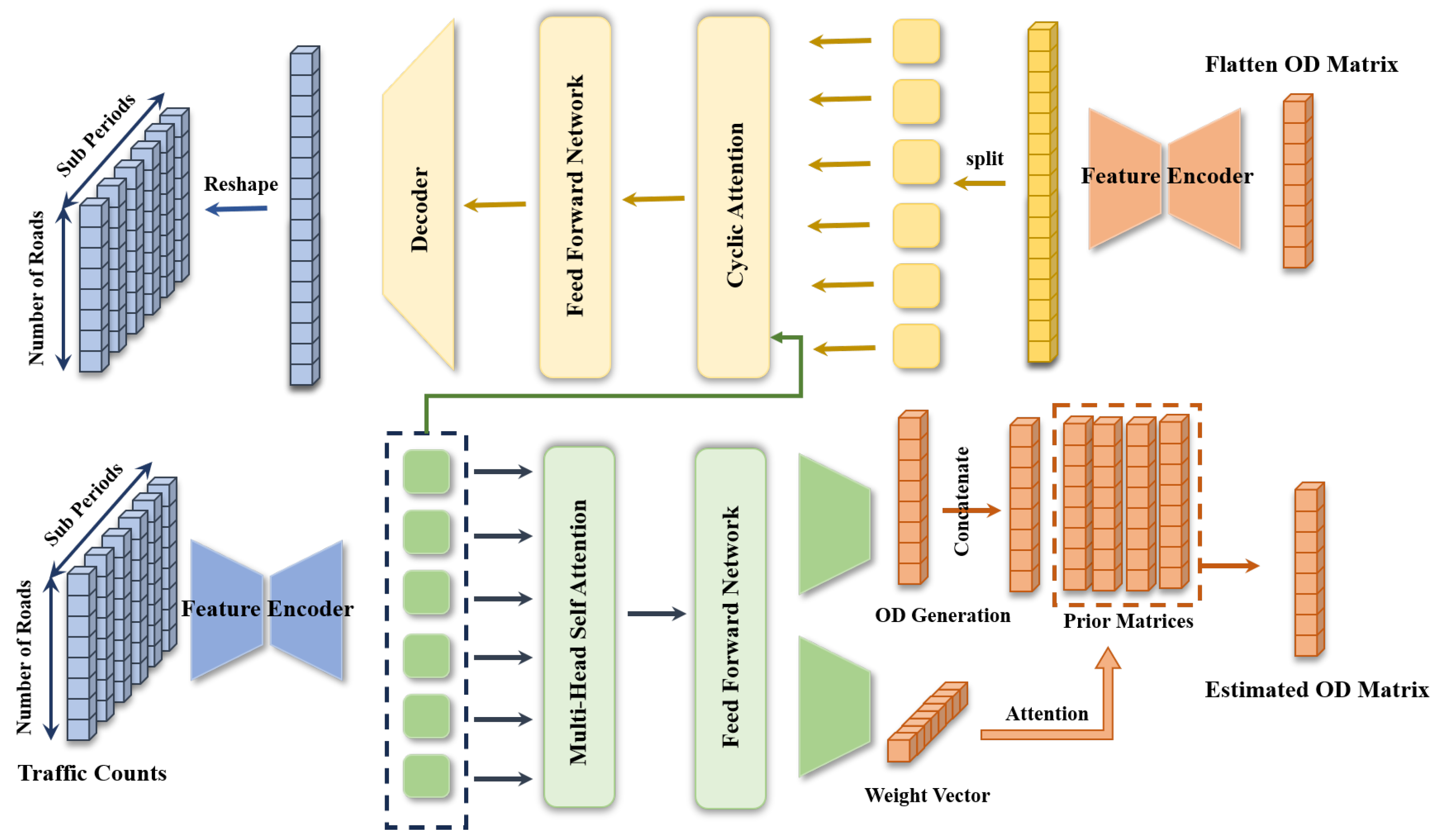
• We find that the self-attention mechanism based on the quasi-dynamic assumption can estimate OD matrices accurately, and based on this, we propose the CQDFormer.
• We design a cyclic attention mechanism that suppresses unrealistic OD estimation due to distribution shift and prevents the degradation of model performance.
• We carry out experiments on a realistic road network to illustrate the validity of the proposed OD estimation method and model, and the results show that the proposed model outperforms all comparison models in the relevant metrics.

The rest of this article is organized as follows. Chapter Two reviews related works on OD estimation. Chapter Three conceptualizes the quasi-dynamic OD estimation problem. Chapter Four details the methodology of CQDFormer. In Chapter Five, the proposed model is evaluated with baseline models in two scenarios. Chapter Six summarizes the entire article.

2. Literature Review

2.1. Data Sources for OD Estimation

Traffic counts are the earliest and most fundamental data in OD estimation [21,22]. Nevertheless, much of the information about trips, including route choice, departure, and arrival time, is not directly reflected in traffic count data. With the development of big data in the era of ITS, much additional data are being used to improve the accuracy of OD estimation, including data from automatic vehicle identification (AVI) [3,23,24], Bluetooth MAC scanner [13], mobile device and GPS [25,26], floating cars [10,27], and smart card records [28].

AVI and Bluetooth-scanning data gather the vehicle identification information and corresponding timestamps. By re-identifying the same vehicle at another location after the initial identification, complete or partial travel path information of the vehicle can be obtained. Recent work has pointed to the existence of a minimum sampling rate that guarantees estimation accuracy using AVI data [24]. The sampling rate is restricted by deployment of roadside AVI devices, the penetration rate of vehicle-side devices, and the accuracy of identification, making it challenging to achieve the desired accuracy in many cities.

Mobile device data includes cellular signaling token [26] and mobile positioning data [29]. It is frequently employed in crowd mobility modeling thanks to the high coverage of cellphones [30]. However, when applying mobile device data to the OD estimation, there are challenges of matching cellphone users with specified roads and traffic modes, and trade-offs between coarse spatial–temporal resolution and privacy protection.

Floating Car Data (FCD) contains detailed spatio-temporal trajectories of a subset of vehicles in the road network, typically from taxis equipped with positioning systems. As a sample of the complete traffic flows, the OD matrix from FCD can be scaled up in a statistical sense into the OD matrix for the full traffic volume. Additionally, FCD can be availed to obtain traffic status, including road travel times and turning rates at intersections. Nevertheless, FCD might be a biased sampling of the entire traffic flow in time and space, influenced by low penetration rates and operating characteristics [16] (e.g., tendency to gravitate to areas with higher demand; higher nighttime share relative to private cars).

Integrating multiple sources of data in OD estimation is undoubtedly a promising future direction. However, in different cities and application scenarios, the availability and usability of additional data sources are not identical, and integrating multi-source data at different levels of completeness is still challenging. Traffic-count-based OD estimation provides a basic usable solution for different scenarios.

2.2. Constrained Optimization

The solution of the OD matrix can be formalized as a constrained optimization problem. These methods include: Entropy Maximization (EM), Maximum Likelihood Estimation (MLE), and Generalized Least Squares (GLS). In thermodynamics, states with higher entropy are considered to have a higher probability of occurring. Zuylen and Willumsen first introduced the concept of entropy into the OD estimation problem, and expressed the convergence to the most likely demand distribution as entropy maximization [31]. EM establishes clear and intuitive formulas with strong interpretability and can be applied in the absence of a prior matrix. It reaches high accuracy in static OD estimation, but is hard to extend to dynamic OD estimation, and the insufficient modeling of dynamics makes the accuracy decrease when the demand structure changes drastically. Different from EM, which considers all states to be equally likely to occur, MLE hypothesizes the prior distribution of OD flows through experience and calculates the most probable states through a Bayesian model [32,33]. The performance of MLE would benefit from an accurate prior probability, but would also be affected by human-induced errors in the prior experience. GLS directly correlates the observations (i.e., traffic counts) and target variables (i.e., OD flows) through the statistical covariance matrix, and minimizes the errors of observations and target variables simultaneously [34,35]. The original model of GLS lacks consideration of the evolution of traffic demand and traffic flow over time and is susceptible to localized noise. To improve the accuracy and stability, dynamic time windows are introduced into GLS with quasi-dynamic assumptions [15]. Since the principles of the groups of optimization methods are similar, they might also be applied in combination. For instance, Xie et al. presented a combined form of EM and least squares, namely EM-LS [36]. A common limitation of this category of models is the homogeneity of traffic demand structure and traffic assignment pattern, both of which tend to be diverse in reality.

2.3. Iterative State Estimations

The iterative state estimation realizes continuous dynamic OD matrix estimation through auto-regressive error control, mainly using Kalman Filter (KF). This branch of methods has been widely explored since Ashok first introduced the concepts [37]. Since the assumption of linear correlation between variables required by ordinary KF is not satisfied in the OD estimation problem, the Extended KF (EKF) and Unscented KF (UKF) apply local linearization to the nonlinear problem by using local derivatives and sample points, respectively. The linearization process causes a considerable computational burden even for medium-size road network [38], and the Local Ensemble Transformed KF (LETKF) reduces the computational complexity by factoring the state variables into several parallellizable sub-states [39]. Inspired by [15], Marzano et al. introduced the quasi-dynamic assumption and presented quasi-dynamic EKF (QD-EKF) to improve the accuracy and stability of dynamic OD estimation [17]. Generally, the Kalman Filter provides an effective tool for tracking dynamic OD matrices, but the large-scale matrix multiplication in it is sensitive to the initial error, and the incomplete accuracy of the parameters (common in OD estimation) tends to result in amplification of the errors and ultimately leads to significant deviations.

2.4. Gradient-Based Estimations

Gradient-based methods include explicit gradient descent (Simultaneous Perturbation Stochastic Approximation, SPSA [40,41,42,43,44,45]) and implicit gradient propagation (Neural Networks, NNs [3,12,19,46,47,48]). As the name suggests, SPSA simultaneously optimizes both the target variable (OD flows) and the observations (traffic count) by gradient descent. Thanks to its simple expression, SPSA can be conveniently deployed in different road networks. However, it is sensitive to OD flows with significant fluctuations, and thus convergence is not guaranteed under large-scale road networks where traffic demand varies significantly. To address this, Tymakianaki et al. clustered OD flows according to their magnitude and assigned a set of hyper-parameters to each cluster [43], which was named c-SPSA. They further presented Robust SPSA to enhance the stability during the gradient process by employing a hybrid gradient strategy [44]. One of the earliest works using neural networks for OD estimation was the Hopfield Neural Networks used in Ref. [46]. Lorenz et al. applied Multi-Layer Perceptron (MLP) to estimate OD matrix [19]. Wu et al. proposed a multi-layered Hierarchical Flow Network to integrate multiple data sources and estimate travel demand [12]. Afandizadeh et al. compared five machine learning methods on OD estimation problems: K-Nearest Neighbor, Random Forest, LightGBM, MLP, CNN [48]. However, as aforementioned, the distribution shift between data of the training set and test set makes the application of neural networks in the field of OD estimation still limited.

3. Problem Statement

Our study aims to dynamically estimate the OD matrix within a reference period given road traffic counts for successive sub-periods. Dynamic OD estimation can be formulated as the solution of Equation (1) as below:

$$f_l\left(t\right)=\sum _{o,d,\tau }{a}_{od\tau }^{lt}{d}_{od}\left(\tau \right)$$

(1)

where the known variable $f_l\left(t\right)$ denotes the traffic counts on road l at time t, and the target variable $d_{od}\left(\tau \right)$ means the number of trips from origin o to destination d departing at time $\tau$. The assignment tensor $a_{od\tau }^{lt}$ establishes a correlation between $d_{od}\left(\tau \right)$ and $f_l\left(t\right)$. However, since both $d_{od}\left(\tau \right)$ and $a_{od\tau }^{lt}$ are unknown, the OD estimation is severely under-determined. To make the problem solvable, we aggregate OD flows along dimension $\tau$ and assume the demand stays stable within the specified period T, that is the quasi-dynamic assumption.

$$d_{od}\left(T\right)=\sum _{\tau \in T}{d}_{od}\left(\tau \right)$$

(2)

The period T can be divided into $n_t$ sub-periods: $T=T_1\cup T_2\cup \cdots \cup T_{n_t}$, and the traffic counts can be aggregated into different sub-periods as Equation (3).

$$f_l\left(T_i\right)=\sum _{t\in T_i}{f}_l\left(t\right)$$

(3)

Based on that, we define quasi-dynamic OD matrix $D_T:=\left[d_{od}\left(T\right)\right]\in {\mathbb{R}}^{n_p\times n_p}$ where $n_p$ denotes the number of traffic analysis zones, and traffic count matrix $F_T:=[f_l\left(T_1\right),f_l\left(T_2\right),f_l\left(T_3\right),\cdots ,f_l\left(T_{n_t}\right)]\in {\mathbb{R}}^{n_l\times n_t}$ where $n_l$ is the number of roads with traffic flow detection. In this article, we intend to estimate $D_T$ through $F_T$.

4. Methodology

Given the $n_p$ traffic analysis zones $\mathbb{P}=\{P_1,P_2,\cdots ,P_{n_p}\}$ and $n_l$ roads $\mathbb{L}=\{l_1,l_2,\cdots ,l_{n_l}\}$, a trip from origin to destination can be written as $P_{{\phi }_o}\to l_{{\alpha }_1}\to l_{{\alpha }_2}\to \cdots \to l_{{\alpha }_{\eta }}\to P_{{\phi }_d}$, with $P_{{\phi }_o}\in \mathbb{P}$ and $l_{{\alpha }_1},\cdots ,l_{{\alpha }_{\eta }}\in \mathbb{L}$. With regard to the temporal dimension, the sub-period when the trip passes $l_{{\alpha }_i}$ is marked as $T_{{\beta }_i}$, in this form, the spatiotemporal trajectory of a trip is expressed as below:

$$r_k:=P_{{\phi }_o}\to \left(l_{{\alpha }_1},T_{{\beta }_1}\right)\to \left(l_{{\alpha }_2},T_{{\beta }_2}\right)\to \dots \to \left(l_{{\alpha }_{\eta }},T_{{\beta }_{\eta }}\right)\to P_{{\phi }_d}$$

(4)

Defining the state of arriving at road $l_{{\alpha }_i}$ at moment $T_{{\beta }_i}$ as $A_i=(l_{{\alpha }_i},T_{{\beta }_i})$, then each element in $F_T$ can be written as Equation (5). When the spatiotemporal trajectory $r_k$ passes through $l_{{\alpha }_i}$ in subperiod $T_{{\beta }_i}$, the trajectory $r_k$ contains state $A_i$ and ${\delta }_{A_i\in r_k}$ equals to 1 otherwise 0. The total number of trajectories containing the state $A_i$ determines the value of $F_T[{\alpha }_i,{\beta }_i]$ together, and the number of trajectories $N\left(r_k\right)$ is related to distribution of path selection and traffic demand structures through Equation (6), where the OD pair form traffic analysis zone $P_m$ to zone $P_n$ has $\gamma$ candidate trajectories $r_k$, and ${\delta }_{{\phi }_o,m}$ and ${\delta }_{{\phi }_d,n}$ indicate the origin and destination of $r_k$ are $P_m$ and $P_n$, respectively. From the above description, it can be seen that the traffic flow matrix $F_T$ and traffic demand matrix $D_T$ are correlated through the spatiotemporal trajectory distribution, and their correlation can be given by Equation (7), where $P\left(r_k\right)$ indicates the probability of selecting the trajectory $r_k$ among all candidate trajectories between origin ${\phi }_o$ and destination ${\phi }_d$.

$$F_T[{\alpha }_i,{\beta }_i]=N\left(A_i\right)=\sum _{r_k}N\left(r_k\right){\delta }_{A_i\in r_k}$$

(5)

$$D_T[m,n]=\sum _{k=1}^{\gamma }N\left(r_k\right){\delta }_{{\phi }_o,m}{\delta }_{{\phi }_d,n}$$

(6)

$$F_T[{\alpha }_i,{\beta }_i]=\sum _{{\phi }_o,{\phi }_d}\sum _{r_k}{D}_T[{\phi }_o,{\phi }_d]P\left(r_k\right){\delta }_{A_i\in r_k}$$

(7)

However, the coupling of temporal and spatial dimensions in $r_k$ and the sharing of multiple trajectories for the same state $A_i$ make the equation groups from Equation (7) hard to resolve explicitly. From Equation (7), the known variables $F_T$ and target variables $D_T$ are related through a series of distribution probabilities, and neural networks are powerful tools for capturing mapping relationships from known distributions to target distributions. We adopt a bidirectional encoder–decoder architecture to approximate the mapping relationship, with forward network estimating OD matrix and backward network assigning traffic flows, as illustrated in Figure 1.

In the forward encoder, each column vector $F_T[:,{\beta }_i]$ in $F_T$ contains information about the spatial distribution of traffic flow in each subperiod, and they are embedded individually to feature space with dimensions of $n_f$ while maintaining the temporal dimension, and produces $n_t$ feature vectors, where $n_t$ is the number of subperiods. The embedded layer applies two fully connected layers as Equation (8).

$$FC\left(x\right)=activation(xW+b)$$

(8)

where x is the input data (here is $F_T$), and W, b are learnable parameters. Here, LeakyReLU, an extension of Rectified Linear Unit (ReLU), is used as the activation function.

Since different $r_k$ contains not exactly the same sequence of states $\left[A_i\right]$, different distributions of $r_k$ lead to various spatiotemporal distributions of traffic flows. Under the quasi-dynamic assumption, this is reflected in the generation of various $F_T$. Meanwhile, the spatiotemporal trajectories $r_k$ connect different origins and destinations, and the distribution of $r_k$ is also associated with the distribution of traffic demand simultaneously. Self-attention mechanism allows models to establish connections between multiple positions within a sequence of data and capture their contextual relationships, and is applied here to extract the association weights between the spatial feature vectors in $n_t$ subperiods, as a way to implicitly represent the probability distribution of $r_k$, and thus map different spatiotemporal flow distributions to different types of traffic demand structures. Because the $n_t$ feature vectors do not explicitly contain sequential information, the position embedding is operated first as in [49].

$$Attention(Q,K,V)=softmax\left(\frac{Q{K}^T}{\sqrt{d_k}}\right)V$$

(9)

$$FFN\left(x\right)=ReLU(x{W}_1+b_1)W_2+b_2$$

(10)

$$AN\left(x\right)=LayerNorm(x+Sublayer(x\left)\right)$$

(11)

Equation (9) is the core formula of self-attention, where $Q,K,V$ are query, key, and value matrices, which are generated from the embedded feature vectors through three different linear transformations. The scaled dot product of Q and K scores the correlation degree between feature vectors in $n_t$ subperiods, where the scaling factor $1/\sqrt{d_k}$ prevents the influence of vector dimensions. The activation function $softmax$ normalizes the dot product of Q and K to indicate the importance weights of value vectors in V. In multi-head attention, each attention head performs attention operation upon a corresponding group of $Q,K,V$ to capture multiple association patterns. The Feedforward Layer deploys two fully connected layers to enhance the nonlinearity of the attention outcome as expressed in Equation (10). The Add&Norm establishes residual connections between the front and back of each sublayer (i.e., Attention layer, Feed Forward layer) and avails layer normalization to improve the performance as in Equation (11).

Encoded by the self-attention module, the feature vectors are fed into two separate decoders. One of them extracts the distributional features of the OD matrices directly from the training data and produces a tensor ${\widehat{D}}_T^{\prime }$ sharing the same dimension with the OD matrix through two fully connected layers. The other produces the weight vector $W_D$ of candidate OD matrices including the OD matrix from the last one decoder ${\widehat{D}}_T^{\prime }$ and $n_d$ prior OD matrices $D_1,D_2,\cdots ,D_{n_d}$, then the final estimation matrix is expressed as

$${\widehat{D}}_T=concat{({\widehat{D}}_T^{\prime },D_1,D_2,\cdots ,D_{n_d})}^T·W_D$$

(12)

Since ${\widehat{D}}_T^{\prime }$ generated mainly from the training of pairwise simulation data is susceptible to distributional shift, the weight tensor $W_D$ receives the gradient backpropagation from the loss of cyclic consistency training with the realistic data and adaptively adjusts the weights to capture the structure of the OD matrix in the real environment.

The inputs of the backward network are a batch of flattened OD matrices. The feature encoder first maps the OD matrix to a $n_t·n_f$-dimensional feature space, where $n_f$ is the feature space dimension of the forward process and $n_t$ is the number of sub-periods. Then, the $n_f\times n_t$ dimensional feature vectors are reshaped into $n_t$ vectors with dimensions of $n_f$, and both feature vectors from forward and backward networks are fed into the cyclic attention module. In the cyclic attention module, the forward embedded feature vector is mapped to query matrix Q and key matrix K, and the backward embedded feature vector is mapped to value matrix V, and the same operation is conducted through Equation (9).

The training data for CQDFormer includes realistic traffic count data and paired simulation data configured from the prior demand matrices and real traffic states. The training process consists of two parts, where independent losses for forward and reverse processes are computed separately for the paired simulation data indicated by the yellow lines in Figure 2. Because the realistic OD matrix is difficult to be accessed in real-time, the training is constrained by cyclic consistency, represented by the blue line in Figure 2. The optimization objective for training can be represented as

$$J=mi{n}_{\theta }\left[D_1(f_{\theta }\left(x_i\right),y_i)+w{D}_2(g_{\alpha }(f_{\theta }\left(x_j\right),x_j)\right]$$

(13)

$D_1,D_2$ are distance measure functions between variables, $f_{\theta }$ is the forward network for OD estimation, and $g_{\alpha }$ is the backward network for traffic assignment, where $\theta$ and $\alpha$ are learnable parameters.

Figure 2. The training process. The proposed CQDFormer consists of forward and backward transformers, the paired simulation data are used for training the forward and backward process, respectively, and the real traffic count data are for training in the cyclic process.

Figure 2. The training process. The proposed CQDFormer consists of forward and backward transformers, the paired simulation data are used for training the forward and backward process, respectively, and the real traffic count data are for training in the cyclic process.

Because traffic count-OD paired data are often missing in real environments, the training data for neural networks need to be expanded by simulation, but uncalibrated simulation data tend to cause an obvious distribution shift between training and evaluation, thus the simulation needs to be calibrated first according to the data obtained in real environments. As illustrated in Figure 3, the prior OD matrices can be derived from historical data, roadside surveys and questionnaires, empirical models (e.g., gravity model), and license plate recognition. In the era of ITS, the prior matrices can also be derived through other estimation models based on multiple data sources. It is worth noting that since these data sources are not necessarily available in real time, these models may not be used for OD estimation at any time, but the historical data generated by these models can be used for simulation calibration. In this study, we do not model the process of obtaining the prior matrices, but select 20 data samples from the test set as the prior matrices. Between each OD pair, we avail depth-first search combined with spatial direction information to obtain 200 paths, and choose all paths whose lengths are less than 1.3 times that of the shortest path as candidate paths between the OD pair.

In the simulated traffic assignment, we consider three types of path selection patterns:

• Fixed Path Selection Pattern. For some familiar travel situations, travelers will tend to choose fixed travel paths. In this path selection path, the probability that a traveler chooses each path is related to the road conditions the path passes, the urban functional areas along the road, etc., and is fixed in each round of simulation.
• N Shortest Path Selection Pattern [47]. Travelers dynamically adjust their path selection according to the traffic states, but subject to information delays, personal preferences, and other factors, ultimately travelers will choose one of the N paths with the shortest travel time, and the probability of choosing each path is related to the level of congestion perceived by the travelers.
• Roaming Path Selection Pattern. This path selection pattern is used to fill in the travel path selection pattern that cannot be described by the two above, including trips without specific purposes or travelers with multiple travel purposes, and the paths in this pattern are generated from all the candidate paths between the origin and the destination.

First, we perform a calibration on the proportion of each path selection mode in the DTA model. Specifically, we arrange the proportions of the three path selection from 0 to 1 in a gradient of $0.1$ to obtain 55 combinations (e.g., (0.2, 0.5, 0.3), (0.2, 0.6, 0.2), etc.), for each prior matrix, we perform 10 rounds of simulation, the traffic count data generated from the j-th round simulation of i-th combinations on the p-th prior matrix is denoted as ${\widehat{F}}_T(i,p,j)$, and we calculate the Manhattan distance between the ${\widehat{F}}_T(i,j)$ to the corresponding traffic count data $F_T\left(p\right)$. We select the parameter combination that minimizes the sum of the differences between ${\widehat{F}}_T(i,p,j)$ and $F_T\left(p\right)$ as the initial configuration. In each round of simulation, the meta-model parameters of DTA fluctuate stochastically within a range of $0.2$.

$$R_{opt}=argmi{n}_i(\sum _{p}mi{n}_j|{\widehat{F}}_T(i,p,j)-F_T\left(p\right)\left|\right)$$

(14)

The prior OD matrices cover the traffic demand in six periods, including morning, morning peak, noon, afternoon, evening peak, and night. In each round of simulation, we perform simulations for these six periods, respectively. For each period, we randomly select a prior OD matrix $D_{main}$ as the main demand structure, and select the traffic count data of the corresponding period from the real data set to perform OD estimation using one or more coarse OD estimations (c-SPSA is used here) to generate an additional OD matrix $D_{sub}$, then the OD matrix for each round of simulation can be calculated as Equation (15)

$$D_T=(D_{main}\times 0.8+D_{sub}\times 0.2)\times normal(0.8,1.2)$$

(15)

where $normal (0.8,1.2)$ means a normal distribution from 0.8 to 1.2. This formula uses combination and randomization to generate as diverse a simulated traffic demand as possible. The OD matrix for simulation is then input into the calibrated DTA model to produce the corresponding traffic count data. We first cluster the real traffic count data for different time-of-days using Gaussian mixture models (GMM), and exclude the out-of-cluster data generated by each simulation. We also apply GMM to cluster the traffic count data generated by simulations, and use probability weight to preferentially sample the real traffic count data that are not in the clusters of simulation data to enhance diversity.

5. Experiments

5.1. Experiment Configuration

The proposed model is evaluated in a realistic urban road network in Haikou, China. On the widely used microscopic traffic simulator, SUMO, we run two independent simulations in parallel, representing the realistic traffic scenario and the simulation used to generate paired OD–traffic count data, respectively. From the “realistic” simulation, the estimation model obtains several prior OD matrices, and real-time traffic counts on the monitored roads, then infers the real hourly OD matrix.

The experimental road network is selected from downtown Haikou city, including 2328 roads and 1171 junctions, of which 359 major arterials are equipped with traffic count detection devices to measure the number of vehicles passing through these roads. Vehicles entering and exiting these roads every five minutes are aggregated into a traffic count vector for a subperiod. The entire network covers an area of 10 km × 6 km and is divided into 31 traffic analysis zones (TAZs), as illustrated in Figure 4. All origin and destination nodes are aggregated in these TAZs, and TAZ might have more than one origin and destination node. Due to the limited size of TAZ, we do not consider the intra-TAZ traffic demand of vehicles, and the OD flows between TAZs make up the elements on the OD matrix. Figure 5 illustrates how traffic demand varies over a day, where blue circles represent the traffic demand in specified hours in each round of the simulation, the orange line represents the hourly average traffic demand on weekdays, and the green line is for weekends.

In the temporal dimension, traffic demand involves two characteristics: time-of-day and day-of-week. The former describes the intra-day fluctuations including six periods: morning, morning peaks, noon, afternoon, afternoon peaks, and night; and the latter consists of weekdays and weekends. In different periods, different intensities of OD flows are generated between TAZs with different attributes (e.g., the significant traffic flows from the residential area to the workplace in the weekday morning peak). Note that multiple attributes may exist in the same TAZ.

As discussed in the last chapter, we set up three ways of path selection in realistic traffic scenarios, where the proportion of these three path selection methods varies between different OD methods and changes over time, and this information about path selection remains unknown to the other simulation used to generate the training data augmentation. To reproduce the diversity of vehicle dynamics in the realistic road network, five categories of vehicles with different dynamics parameters are set up in the simulation: normal cars, conservative cars, aggressive cars, buses, and trucks.

Each round of “realistic” simulation lasts $17.3$ simulation hours, from 5:20 a.m. to 10:40 p.m. With regard to the simulation stabilization process, the warm-up and cool-down times of 40 m are not used for estimation. The simulation is executed for 600 rounds, generating 600-day data including 172 weekends and 428 weekdays. Additional 4000-round paired data are generated by the parallel simulation, of which each round includes 2 h each of the above 6 periods, and the half-hours of warm-up and cool-down are not recorded. The specific parameters of the experiment are given in

Table 1. Parameter configuration.

Categories	Parameters	Values
Simulation for	Epoch Number for Realistic Data	600 epoch
Realistic Environment	Simulation Duration for Realistic Data	17.3 h/epoch
	Path Selection Ratio	(0.35, 0.53, 0.12)
Simulation for	Epoch Number for Paired Data Generation	4000 epoch
Data Generation	Simulation Duration for Paired Data Generation	12 h/epoch
	Path Selection Ratio	(0.4, 0.5, 0.1)
	Number of Prior OD Matrices	20
Model Parameters	Epoch Number for Training	100
	Batch Size	16
	Sequence Length of Attention	12
	Head Number of Attention	3
	Dimensions of feature space	150
	Dimensions of Query, Key, Value Matrices	50
	Hidden Dimensions for forward Networks	256
	Hidden Dimensions for backward Networks	1024
	Optimizer	Adam
	Learning Rate	0.0001
	Decay of Learning Rate	0.2/10 epochs

.

5.2. Evaluation Metrics

Four metrics are used to evaluate the performance of the proposed and comparison methods in the experiment [1,16,24,43,50].

• Root Mean Square Error (RMSE)

  $$RMSE=\sqrt{\frac{1}{N}\sum _{i=1}^N\left|\right|Y_i-{\widehat{Y}}_i{\left|\right|}_2^2}$$

  (16)
• Mean Absolute Error (MAE)

  $$MAE=\frac{1}{N}\sum _{i=1}^N\left|Y_i-{\widehat{Y}}_i\right|$$

  (17)
• Mean Absolute Perceptage Error (MAPE)

  $$MAPE=\frac{1}{N}\sum _{i=1}^N\frac{|Y_i-{\widehat{Y}}_i|}{|Y_i|}\times 100\%$$

  (18)
• Coefficient of Determination ($R^2$)

  $$R^2=1-\frac{{\sum }_{i=1}^N\left|\right|Y_i-{\widehat{Y}}_i{\left|\right|}_2^2}{{\sum }_{i=1}^N\left|\right|Y_i-\overline{Y}{\left|\right|}_2^2}$$

  (19)

where N denotes the number of samples in the evaluation dataset, $Y_i$ means the true hourly OD matrix, ${\widehat{Y}}_i$ is the corresponding estimation matrix, and $\overline{Y}$ is the average of $Y_i$. The operators $|·|$, $\left|\right|·{\left|\right|}_2$ denote L1 and L2 norms.

The RMSE and MAE measure the absolute errors between the OD matrix and its estimation, and MAPE quantifies the relative error. $R^2$ compares the estimation error to the fluctuation from the average of the data, and the closer it is to 1, the better the model performs.

5.3. Comparison Model

We select four benchmark methods for comparison, two advanced OD estimation methods and two learning-based methods. The c-SPSA and EKF are the most typical models in the two major categories of methods estimating OD matrix from traffic count (Gradient-based Estimation, Iterative State Estimation). Since this study explores OD estimation under multiple demand structures and implements diversified traffic assignment modes, it is hard to deploy the Constrained Optimization method here, which is more theoretical. As far as the author knows, MLP is the earliest and most widely used model that applies neural networks to the field of OD estimation. Since CycleGAN is one of the earliest works to apply cyclic consistency in neural networks and inspires the design of the proposed model, it is also used here as a comparative experiment.

• Cluster-SPSA(c-SPSA), an effective way to cope with multiple magnitudes of OD flows. Referring to [43], the number of clustering kernels is set to 3.
• Extended Kalman Filter (EKF), a non-linear extension of Kalman Filter, shows promising performance in arterial network [17].
• Multi-Layer Perceptron (MLP), a widely used neural network block, was applied to the OD estimation in [19,48]. Here, we use the encoder–decoder framework including six linear transformation layers with dimensions of $1024,512,256,256,512,1024$, respectively, and the LeakyReLU is used as the activation function between layers. The encoder–decoder framework can realize effective feature compression and extraction through dimensionality reduction.
• Cycle Generative Adversarial Networks (CycleGAN), one of the first works to introduce the concept of cyclic consistency, with notable success in the field of stylized image generation [51]. The proposed model is inspired by and incorporates the concept of cyclic consistency, thus we use this model as a comparison model.

5.4. Results and Discussion

5.4.1. Performance Evaluation

The performance of CQDFormer and comparison models is presented in

Table 2. Performance comparison.

	c-SPSA	EKF	MLP	CycleGAN	Proposed
RMSE	9.0643	22.2006	7.8831	11.1776	4.1796
MAE	6.9656	13.5181	5.5624	6.9010	3.0373
MAPE	24.78%	59.44%	14.38%	18.99%	10.10%
$R^2$	0.5778	-0.0341	0.6536	0.4793	0.8053

, and the proposed model achieves the best in all four metrics. The RSME and MAE intuitively reflect the difference between the estimated and true OD matrices, and the RMSE and MAE of the proposed model are 4.1796 and 3.0373, which are $46.98\%$ and $45.40\%$ improved compared to the MLP, and $53.89\%$ and $56.40\%$ improved compared to the c-SPSA. MAPE, on the other hand, portrays the relative accuracy of the models, and since the magnitude of OD flows has large variations from location to location and time to time, and commonly the higher the magnitude of the OD flow reaches, the larger the error is, MAPE provides a relatively fairer metric. The MAPE of the proposed model is $10.10\%$, showing a performance improvement of $29.76\%$ and $46.81\%$ with respect to MLP and CycleGAN. The $R^2$ measures the coefficient of determination of models, and it varies from negative infinity to 1, with better performance the closer it is to 1. When $R^2$ takes a positive value, it indicates the model is better than the simple and direct method (i.e., averaging all data directly), so in many cases, only $R^2$ between 0-1 is considered meaningful. Nevertheless, the presence of negative $R^2$ in this experiment is reasonable because the average of realistic OD matrices actually remains unknown. The $R^2$ of the proposed model is equal to $0.8053$, being the highest among all models, and the MLP is the next highest, equal to $0.6536$.

5.4.2. Results of Traffic Assignment Simulation

As mentioned previously, two parallel simulations are used in the experiment, where one simulation represents the real scenario and the other is used to establish a simulation-based dynamic traffic assignment model and generate pairwise data for neural network training. There are three types of path selection as mentioned in the last chapter: fixed, efficient, and random, and the ratio of these three for the “real traffic” simulation is $[0.35,0.53,0.12]$. The calibrated simulation-based DTA model obtains the ratio of these three as $[0.4,0.5,0.1]$. Figure 6 illustrates the relationship between the average 5-min flow per hour between these two simulations.

5.4.3. Computational Cost

The experiments are conducted on a computer with a 12-core i7-12700KF @4.9GHz/RAM: 32 GB processor and NVDIA 3080. Training Time and Evaluation Time. The running time of real environment simulation and simulation for training data generation are 5 days and 20 days, respectively. The parameter number of CQDFormer is $14M$ and its training time and evaluation time are 2 h and 2 ms, respectively.

5.4.4. Result Analysis

In this section, we will analyze the superiority of the proposed model against other baselines as shown in Section 5.4.1. Figure 7 and Figure 8 further display the comparison results in an intuitive visual manner. In Figure 7, ten thousand pieces of data in the evaluation dataset are randomly selected, where the x-axis represents the true value of OD flow and the y-axis represents the estimated value of the model. The standard line at 45 degrees stands for a perfectly accurate estimation. The closer the state points are to the standard line, the better estimations they stand for. Figure 8 illustrates the dimensionality reduction using Principal Component Analysis (PCA), where the first two principal components are plotted [52,53,54,55,56]. Each density peak and its respective cluster in can be regarded as a type of traffic demand structure. The traffic demand structure is defined as the distribution pattern of traffic demand between different OD pairs and reflects the fundamental skeleton of the dynamic OD matrix [57,58].

The daily travel activities of urban residents have multiple types of attributes, including work, leisure, shopping, and more. These travel attributes may lead to different traffic demand structures at different time and scenarios [59]. As shown in Figure 8a, the real road network used for conducting simulation contains multiple traffic demand structures. Diverse traffic demand structures may contain various travel patterns [60] and generate different traffic states (e.g., congested and un-congested state) and evolutionary patterns [61], and further affect the accuracy of OD estimation [62]. Figure 8b–f show the capability of each model to capture those traffic demand structures. More specifically, the more completely the model captures these structures, the more accurate the model’s estimation is likely to be.

According to Figure 7 and Figure 8, the models taking multiple traffic structures into account tend to present higher estimation accuracies. Both c-SPSA and learning-based methods implicitly or explicitly include the information about multiple traffic demand structures. The Extended Kalman Filter captures the time-dependent traffic demand patterns by capturing the evolutionary characteristics of traffic demand and states over time [17,63,64]. It presents promising results when there are a homogeneous and significant traffic demand evolution pattern, which is suitable for the OD estimation problem in an arterial road or a network composed of several arterial roads. Nevertheless, in the presence of multiple traffic demand evolution patterns, the Kalman Filter might fail to track the trend of traffic demand in a real urban network, and the estimated OD matrices might cluster around the single prior traffic demand structure, as illustrated in Figure 8f. The explicit gradient-based estimation model, SPSA, introduces a prior OD matrix as the structural skeleton of the estimated OD matrices [40]. In order to capture the structural information of traffic demand more accurately, weight-SPSA (W-SPSA) and cluster-SPSA (c-SPSA) have been successively proposed [43,65,66]. Therein, c-SPSA provides a stable gradient strategy by clustering the traffic demand of different intensities with a specific set of hyperparameters for each cluster to accommodate OD estimation under multiple demand structures. However, due to the absence of correlation mappings from a traffic evolution pattern to the corresponding demand structure in model, the estimation results of c-SPSA are susceptible to the influence of the prior matrices and noises of DTA process, which can lead to the failure of capturing some non-significant demand structures.

Neural networks excel in discovering multiple implicit patterns in the target distributions through feature extraction of the data and enable us to establish many-to-many mappings between known distributions (traffic counts) and target distributions (OD matrices). As can be seen in Figure 8, CQDFormer and MLP basically capture complete traffic demand structures in the real data set. This is one of the main reasons why they can outperform other baselines and achieve minimal dispersion in Figure 7. However, MLP has relatively poor performance in capturing low-density traffic structures due to the distribution shift. In contrast, as observed in Figure 8e, cyclic consistency improves the coverage of the estimation with respect to the low-density clusters, but since the GAN focuses more on capturing the distribution of the data rather than the exact OD values, making the OD matrices generated by CycleGAN discrete and not precise enough. CQDFormer introduces cyclic consistency along with the use of a prior matrices to anchor the demand structures, and realizes the accurate mapping from a specific spatio-temporal evolutionary pattern to the corresponding demand structure through the self-attention mechanism. The above results and discussion demonstrate the competence of the proposed model in the OD estimation problem in complex urban environment.

5.4.5. Convergence

Figure 9a shows the training process of three neural networks, MLP, CycleGAN, and CQDFormer. The learning rates of the three neural networks are chosen to be $0.0005$, $0.0005$, and $0.0001$, respectively. The training process consists of 30,000 iterations, with the batch size of sampled data being 16. Before training, the mean and standard deviation of the training data are both normalized to 1. During training, the loss of CycleGAN has relatively dramatic fluctuations and reaches around $0.8$ eventually. Both MLP and CQDFormer converge rapidly in the early stages of training, with MLP converging to $0.0566$ around 3000 rounds and CQDFormer converging to $0.0907$ around 5000 rounds. Cyclic consistency restricts further descent of the CQDFormer to prevent it from overfitting the training set. A total of 3600 rounds of cyclic consistency are trained on the real data and converge to $0.07$ around 3000 rounds, as illustrated in Figure 9b.

6. Conclusions

Dynamic origin–destination estimation is an important and challenging problem due to its under-determination and high non-linearity. By introducing the quasi-dynamic assumption, this paper proposes an effective attention-based neural network, called CQDFormer. The proposed CQDFormer consists of forward and backward transformers, where the forward transformer performs OD estimation and the backward one approximates the traffic assignment process. The correlations between traffic count vectors for each sub-period are extracted by the self-attention modules to capture path selection information and used in the learning process in both directions. During the training process, the data generated by the simulation is used for separate training of forward and backward learning, while the real traffic count data are used for training of cyclic consistency to calibrate the differences between the simulation and the real environment.

We evaluate the effectiveness of CQDFormer through a real urban road network in Haikou, China. In the experiments, we find that the quasi-dynamic assumption can effectively address the under-determination challenge in OD estimation. Accurate generation of OD matrices can be achieved through traffic count vectors in multiple sub-periods, and gradient-based methods, such as neural networks, have strong estimation capabilities in this process. Particularly, the proposed CQDFormer converges quickly and achieves outstanding results in RMSE, MAE, MAPE, and $R^2$ compared with the benchmark methods. We select 10,000 OD flows to plot the correspondence between the estimated values and the real values, which shows that CQDFormer can achieve excellent estimation of OD flows of different magnitudes and has the potential to be applied in various traffic states—both congested and uncongested states.

The limitation of this study is that the current data-driven OD estimation method suffers from dependence on specific road topology scenarios, and the process of data generation and training has to be repeated for the application under different road networks, which will be a time-consuming process. Future research can attempt to introduce the road structure into OD estimation frameworks through graph neural networks.

References

1. Ou, J.; Lu, J.; Xia, J.; An, C.; Lu, Z. Learn, assign, and search: Real-time estimation of dynamic origin-destination flows using machine learning algorithms. IEEE Access 2019, 7, 26967–26983. [Google Scholar] [CrossRef]
2. Sun, W.; Shao, H.; Shen, L.; Wu, T.; Lam, W.H.; Yao, B.; Yu, B. Bi-objective traffic count location model for mean and covariance of origin–destination estimation. Expert Syst. Appl. 2021, 170, 114554. [Google Scholar] [CrossRef]
3. Cao, Y.; Tang, K.; Sun, J.; Ji, Y. Day-to-day dynamic origin–destination flow estimation using connected vehicle trajectories and automatic vehicle identification data. Transp. Res. Part C Emerg. Technol. 2021, 129, 103241. [Google Scholar] [CrossRef]
4. Guo, J.; Liu, Y.; Li, X.; Huang, W.; Cao, J.; Wei, Y. Enhanced least square based dynamic OD matrix estimation using Radio Frequency Identification data. Math. Comput. Simul. 2019, 155, 27–40. [Google Scholar] [CrossRef]
5. Tang, K.; Cao, Y.; Chen, C.; Yao, J.; Tan, C.; Sun, J. Dynamic origin-destination flow estimation using automatic vehicle identification data: A 3D convolutional neural network approach. Comput.-Aided Civ. Infrastruct. Eng. 2021, 36, 30–46. [Google Scholar] [CrossRef]
6. Montero, L.; Ros-Roca, X.; Herranz, R.; Barceló, J. Fusing mobile phone data with other data sources to generate input OD matrices for transport models. Transp. Res. Procedia 2019, 37, 417–424. [Google Scholar] [CrossRef]
7. Wang, Z.; Wang, S.; Lian, H. A route-planning method for long-distance commuter express bus service based on OD estimation from mobile phone location data: The case of the Changping Corridor in Beijing. Public Transp. 2021, 13, 101–125. [Google Scholar] [CrossRef]
8. Yang, X.; Lu, Y.; Hao, W. Origin-destination estimation using probe vehicle trajectory and link counts. J. Adv. Transp. 2017, 2017, 4341532. [Google Scholar] [CrossRef]
9. Nigro, M.; Cipriani, E.; del Giudice, A. Exploiting floating car data for time-dependent Origin–Destination matrices estimation. J. Intell. Transp. Syst. 2018, 22, 159–174. [Google Scholar] [CrossRef]
10. Mitra, A.; Attanasi, A.; Meschini, L.; Gentile, G. Methodology for O-D matrix estimation using the revealed paths of floating car data on large-scale networks. IET Intell. Transp. Syst. 2020, 14, 1704–1711. [Google Scholar] [CrossRef]
11. Sun, L.; Axhausen, K.W. Understanding urban mobility patterns with a probabilistic tensor factorization framework. Transp. Res. Part B Methodol. 2016, 91, 511–524. [Google Scholar] [CrossRef]
12. Wu, X.; Guo, J.; Xian, K.; Zhou, X. Hierarchical travel demand estimation using multiple data sources: A forward and backward propagation algorithmic framework on a layered computational graph. Transp. Res. Part C Emerg. Technol. 2018, 96, 321–346. [Google Scholar] [CrossRef]
13. Behara, K.N.; Bhaskar, A.; Chung, E. A novel methodology to assimilate sub-path flows in bi-level OD matrix estimation process. IEEE Trans. Intell. Transp. Syst. 2020, 22, 6931–6941. [Google Scholar] [CrossRef]
14. Cipriani, E.; Gemma, A.; Mannini, L.; Carrese, S.; Crisalli, U. Traffic demand estimation using path information from Bluetooth data. Transp. Res. Part C Emerg. Technol. 2021, 133, 103443. [Google Scholar] [CrossRef]
15. Cascetta, E.; Papola, A.; Marzano, V.; Simonelli, F.; Vitiello, I. Quasi-dynamic estimation of o–d flows from traffic counts: Formulation, statistical validation and performance analysis on real data. Transp. Res. Part B Methodol. 2013, 55, 171–187. [Google Scholar] [CrossRef]
16. Bauer, D.; Richter, G.; Asamer, J.; Heilmann, B.; Lenz, G.; Kölbl, R. Quasi-dynamic estimation of OD flows from traffic counts without prior OD matrix. IEEE Trans. Intell. Transp. Syst. 2017, 19, 2025–2034. [Google Scholar] [CrossRef]
17. Marzano, V.; Papola, A.; Simonelli, F.; Papageorgiou, M. A Kalman filter for quasi-dynamic od flow estimation/updating. IEEE Trans. Intell. Transp. Syst. 2018, 19, 3604–3612. [Google Scholar] [CrossRef]
18. Ma, W.; Qian, Z.S. Estimating multi-year 24/7 origin-destination demand using high-granular multi-source traffic data. Transp. Res. Part C Emerg. Technol. 2018, 96, 96–121. [Google Scholar] [CrossRef]
19. Lorenzo, M.; Matteo, M. OD matrices network estimation from link counts by neural networks. J. Transp. Syst. Eng. Inf. Technol. 2013, 13, 84–92. [Google Scholar] [CrossRef]
20. Krishnakumari, P.; van Lint, H.; Djukic, T.; Cats, O. A data driven method for OD matrix estimation. Transp. Res. Procedia 2019, 38, 139–159. [Google Scholar] [CrossRef]
21. Van Zuylen, H. A method to estimate a trip matrix from traffic volume counts. In Proceedings of the PTRC Summer Annual Meeting, Coventry, UK, 11 July 1978. [Google Scholar]
22. Willumsen, L. Estimating the most likely OD matrix from traffic counts. In Proceedings of the 11th Annual Conference of Universities Transport Studies Group, University of Southampton, Southampton, UK, January 1979. [Google Scholar]
23. Zhou, X.; Mahmassani, H.S. Dynamic origin-destination demand estimation using automatic vehicle identification data. IEEE Trans. Intell. Transp. Syst. 2006, 7, 105–114. [Google Scholar] [CrossRef]
24. Rao, W.; Wu, Y.J.; Xia, J.; Ou, J.; Kluger, R. Origin-destination pattern estimation based on trajectory reconstruction using automatic license plate recognition data. Transp. Res. Part C Emerg. Technol. 2018, 95, 29–46. [Google Scholar] [CrossRef]
25. Ma, J.; Li, H.; Yuan, F.; Bauer, T. Deriving operational origin-destination matrices from large scale mobile phone data. Int. J. Transp. Sci. Technol. 2013, 2, 183–204. [Google Scholar] [CrossRef]
26. Iqbal, M.S.; Choudhury, C.F.; Wang, P.; González, M.C. Development of origin–destination matrices using mobile phone call data. Transp. Res. Part C Emerg. Technol. 2014, 40, 63–74. [Google Scholar] [CrossRef]
27. Cao, P.; Miwa, T.; Yamamoto, T.; Morikawa, T. Bilevel generalized least squares estimation of dynamic origin–destination matrix for urban network with probe vehicle data. Transp. Res. Rec. 2013, 2333, 66–73. [Google Scholar] [CrossRef]
28. Munizaga, M.A.; Palma, C. Estimation of a disaggregate multimodal public transport Origin–Destination matrix from passive smartcard data from Santiago, Chile. Transp. Res. Part C Emerg. Technol. 2012, 24, 9–18. [Google Scholar] [CrossRef]
29. Ge, Q.; Fukuda, D. Updating origin–destination matrices with aggregated data of GPS traces. Transp. Res. Part C Emerg. Technol. 2016, 69, 291–312. [Google Scholar] [CrossRef]
30. Phithakkitnukoon, S.; Horanont, T.; Lorenzo, G.D.; Shibasaki, R.; Ratti, C. Activity-aware map: Identifying human daily activity pattern using mobile phone data. In Proceedings of the International Workshop on Human Behavior Understanding, Istanbul, Turkey, 22 August 2010; Springer: Berlin/Heidelberg, Germany, 2010; pp. 14–25. [Google Scholar]
31. Van Zuylen, H.J.; Willumsen, L.G. The most likely trip matrix estimated from traffic counts. Transp. Res. Part B Methodol. 1980, 14, 281–293. [Google Scholar] [CrossRef]
32. Ben-Akiva, M.; Macke, P.P.; Hsu, P.S. Alternative Methods to Estimate Route-Level Trip Tables and Expand on-Board Surveys; Number 1037; National Academies: Washington, DC, USA, 1985. [Google Scholar]
33. Aerde, M.V.; Rakha, H.; Paramahamsan, H. Estimation of origin-destination matrices: Relationship between practical and theoretical considerations. Transp. Res. Rec. 2003, 1831, 122–130. [Google Scholar] [CrossRef]
34. Cascetta, E. Estimation of trip matrices from traffic counts and survey data: A generalized least squares estimator. Transp. Res. Part B Methodol. 1984, 18, 289–299. [Google Scholar] [CrossRef]
35. Bell, M.G. The estimation of origin-destination matrices by constrained generalised least squares. Transp. Res. Part B Methodol. 1991, 25, 13–22. [Google Scholar] [CrossRef]
36. Xie, C.; Kockelman, K.M.; Waller, S.T. A maximum entropy-least squares estimator for elastic origin-destination trip matrix estimation. Procedia-Soc. Behav. Sci. 2011, 17, 189–212. [Google Scholar] [CrossRef]
37. Ashok, K. Dynamic origin-destination matrix estimation and prediction for real-time traffic management system. In Proceedings of the 12th International Symposium on Transportation and Traffic Theory, Berkeley, CA, USA, 21–23 July 1993; pp. 465–484. [Google Scholar]
38. Antoniou, C.; Ben-Akiva, M.; Koutsopoulos, H.N. Nonlinear Kalman filtering algorithms for on-line calibration of dynamic traffic assignment models. IEEE Trans. Intell. Transp. Syst. 2007, 8, 661–670. [Google Scholar] [CrossRef]
39. Carrese, S.; Cipriani, E.; Mannini, L.; Nigro, M. Dynamic demand estimation and prediction for traffic urban networks adopting new data sources. Transp. Res. Part C Emerg. Technol. 2017, 81, 83–98. [Google Scholar] [CrossRef]
40. Balakrishna, R.; Koutsopoulos, H.N. Incorporating within-day transitions in simultaneous offline estimation of dynamic origin-destination flows without assignment matrices. Transp. Res. Rec. 2008, 2085, 31–38. [Google Scholar] [CrossRef]
41. Cipriani, E.; Florian, M.; Mahut, M.; Nigro, M. A gradient approximation approach for adjusting temporal origin–destination matrices. Transp. Res. Part C Emerg. Technol. 2011, 19, 270–282. [Google Scholar] [CrossRef]
42. Balakrishna, R.; Ben-Akiva, M.; Koutsopoulos, H.N. Offline calibration of dynamic traffic assignment: Simultaneous demand-and-supply estimation. Transp. Res. Rec. 2007, 2003, 50–58. [Google Scholar] [CrossRef]
43. Tympakianaki, A.; Koutsopoulos, H.N.; Jenelius, E. c-SPSA: Cluster-wise simultaneous perturbation stochastic approximation algorithm and its application to dynamic origin–destination matrix estimation. Transp. Res. Part C Emerg. Technol. 2015, 55, 231–245. [Google Scholar] [CrossRef]
44. Tympakianaki, A.; Koutsopoulos, H.N.; Jenelius, E. Robust SPSA algorithms for dynamic OD matrix estimation. Procedia Comput. Sci. 2018, 130, 57–64. [Google Scholar] [CrossRef]
45. Ros-Roca, X.; Montero, L.; Barceló, J.; Nökel, K. Dynamic origin-destination matrix estimation with ICT traffic measurements using SPSA. In Proceedings of the 2021 7th International Conference on Models and Technologies for Intelligent Transportation Systems (MT-ITS), Heraklion, Greece, 16–17 June 2021; IEEE: New York, NY, USA, 2021; pp. 1–8. [Google Scholar]
46. Gong, Z. Estimating the urban OD matrix: A neural network approach. Eur. J. Oper. Res. 1998, 106, 108–115. [Google Scholar] [CrossRef]
47. Krishnakumari, P.; Van Lint, H.; Djukic, T.; Cats, O. A data driven method for OD matrix estimation. Transp. Res. Part C Emerg. Technol. 2020, 113, 38–56. [Google Scholar] [CrossRef]
48. Afandizadeh Zargari, S.; Memarnejad, A.; Mirzahossein, H. Hourly Origin–Destination Matrix Estimation Using Intelligent Transportation Systems Data and Deep Learning. Sensors 2021, 21, 7080. [Google Scholar] [CrossRef]
49. Vaswani, A.; Shazeer, N.; Parmar, N.; Uszkoreit, J.; Jones, L.; Gomez, A.N.; Kaiser, Ł.; Polosukhin, I. Attention is all you need. In Attention is all you need. In Proceedings of the Advances in Neural Information Processing Systems, Long Beach, CA, USA, 4–9 December 2017; Volume 30, pp. 5998–6008. [Google Scholar]
50. Tang, J.; Zhang, S.; Chen, X.; Liu, F.; Zou, Y. Taxi trips distribution modeling based on Entropy-Maximizing theory: A case study in Harbin city—China. Phys. A Stat. Mech. Its Appl. 2018, 493, 430–443. [Google Scholar] [CrossRef]
51. Zhu, J.Y.; Park, T.; Isola, P.; Efros, A.A. Unpaired image-to-image translation using cycle-consistent adversarial networks. In Proceedings of the Proceedings of the IEEE International Conference on Computer Vision, Venice, Italy, 22–29 October 2017; pp. 2223–2232.
52. Djukic, T.; Van Lint, J.; Hoogendoorn, S. Application of principal component analysis to predict dynamic origin–destination matrices. Transp. Res. Rec. 2012, 2283, 81–89. [Google Scholar] [CrossRef]
53. Prakash, A.A.; Seshadri, R.; Antoniou, C.; Pereira, F.C.; Ben-Akiva, M. Improving scalability of generic online calibration for real-time dynamic traffic assignment systems. Transp. Res. Rec. 2018, 2672, 79–92. [Google Scholar] [CrossRef]
54. Qurashi, M.; Ma, T.; Chaniotakis, E.; Antoniou, C. PC–SPSA: Employing dimensionality reduction to limit SPSA search noise in DTA model calibration. IEEE Trans. Intell. Transp. Syst. 2019, 21, 1635–1645. [Google Scholar] [CrossRef]
55. Qurashi, M.; Lu, Q.L.; Cantelmo, G.; Antoniou, C. Dynamic demand estimation on large scale networks using Principal Component Analysis: The case of non-existent or irrelevant historical estimates. Transp. Res. Part C Emerg. Technol. 2022, 136, 103504. [Google Scholar] [CrossRef]
56. Fu, H.; Lam, W.H.; Shao, H.; Kattan, L.; Salari, M. Optimization of multi-type traffic sensor locations for estimation of multi-period origin-destination demands with covariance effects. Transp. Res. Part E Logist. Transp. Rev. 2022, 157, 102555. [Google Scholar] [CrossRef]
57. Djukic, T. Dynamic OD Demand Estimation and Prediction for Dynamic Traffic Management. 2014. Available online: https://www.researchgate.net/publication/269575189_Dynamic_OD_Demand_Estimation_and_Prediction_for_Dynamic_Traffic_Management (accessed on 21 July 2023).
58. Behara, K.N.; Bhaskar, A.; Chung, E. A novel approach for the structural comparison of origin-destination matrices: Levenshtein distance. Transp. Res. Part C Emerg. Technol. 2020, 111, 513–530. [Google Scholar] [CrossRef]
59. Katranji, M.; Kraiem, S.; Moalic, L.; Sanmarty, G.; Khodabandelou, G.; Caminada, A.; Hadj Selem, F. Deep multi-task learning for individuals origin–destination matrices estimation from census data. Data Min. Knowl. Discov. 2020, 34, 201–230. [Google Scholar] [CrossRef]
60. Ma, W.; Pi, X.; Qian, S. Estimating multi-class dynamic origin-destination demand through a forward-backward algorithm on computational graphs. Transp. Res. Part C Emerg. Technol. 2020, 119, 102747. [Google Scholar] [CrossRef]
61. Lu, C.C.; Zhou, X.; Zhang, K. Dynamic origin–destination demand flow estimation under congested traffic conditions. Transp. Res. Part C Emerg. Technol. 2013, 34, 16–37. [Google Scholar] [CrossRef]
62. Behara, K.N.; Bhaskar, A. Can partial structural information of travel demand improve the quality of OD matrix estimates? In Proceedings of the Australasian Transport Research Forum, Brisbane, Australia, 8–10 December 2021. [Google Scholar]
63. Van Hinsbergen, C.P.; Schreiter, T.; Zuurbier, F.S.; Van Lint, J.; Van Zuylen, H.J. Localized extended kalman filter for scalable real-time traffic state estimation. IEEE Trans. Intell. Transp. Syst. 2011, 13, 385–394. [Google Scholar] [CrossRef]
64. Barceló Bugeda, J.; Montero Mercadé, L.; Bullejos, M.; Serch, O.; Carmona Bautista, C. A kalman filter approach for the estimation of time dependent od matrices exploiting bluetooth traffic data collection. In Proceedings of the TRB 91st Annual meeting compendium of papers DVD, Washington, DC, USA, 22–26 January 2012; pp. 1–16. [Google Scholar]
65. Lu, L. W-SPSA: An Efficient Stochastic Approximation Algorithm for the Off-Line Calibration of Dynamic Traffic Assignment Models. Ph.D. Thesis, Massachusetts Institute of Technology, Cambridge, MA, USA, 2013. [Google Scholar]
66. Antoniou, C.; Azevedo, C.L.; Lu, L.; Pereira, F.; Ben-Akiva, M. W–SPSA in practice: Approximation of weight matrices and calibration of traffic simulation models. Transp. Res. Procedia 2015, 7, 233–253. [Google Scholar] [CrossRef]
Figure 1. Architecture of CQDFormer. CQDFormer adopts a bidirectional encoder–decoder architecture. It uses self-attention and cyclic attention mechanisms to capture the diverse and nonlinear features of traffic demand and assignment. Feature vectors from both forward and backward networks are fed into the cyclic attention module.
Applsci 13 11257 g001
Figure 3. The flowchart of generating traffic count-OD paired data. Applsci 13 11257 i001 are variables obtained from the real traffic scenario, Applsci 13 11257 i002 are variables generated in the simulation process, and Applsci 13 11257 i003 refers to the processing operations.
Applsci 13 11257 g003
Figure 4. The experimental road network in Haikou City from Open Street Map. The experimental network consists of 31 traffic analysis zones (TAZs), with an area of 10 km × 6 km. The TAZs are selected from the district’s primary areas, such as schools, neighborhoods, commercial districts, and administrative premises.
Applsci 13 11257 g004
Figure 5. The number of trips in different hours. The y-axis displays the normalized proportion of the current traffic demand to the daily average traffic demand. The box-plot represents the traffic demand’s distributional property within the generated 600-day data. The circles are outliers of the box-plot.
Applsci 13 11257 g005
Figure 6. Comparison of real and simulated traffic counts. The 45-degree line represents an ideal estimation. The nearer the state points are to this line, the more accurate the estimates they represent. A total of 10,000 state points are randomly sampled.
Applsci 13 11257 g006
Figure 7. Comparison of real and estimated OD flows.
Applsci 13 11257 g007
Figure 8. Principal component analysis of estimation models. This shows the distribution density of two-dimensional data after dimension reduction through principal component analysis. The domain is uniformly divided into 20 × 20 grids. The distribution density refers to proportion of the number of sample points within each of the grid with respect to the total points.
Applsci 13 11257 g008
Figure 9. The loss curves of neural networks.
Applsci 13 11257 g009