Appendix A
The experimental data and graphs for the remaining four datasets in Experimental
Section 5.1 are shown here.
Figure A1,
Figure A2,
Figure A3 and
Figure A4 depict the classification of anomalous labels under different time windows in the SKAB dataset.
Table A1 presents the detectors selected by our algorithm with comparable performance under different time windows and the preferred detectors when combining multiple time windows.
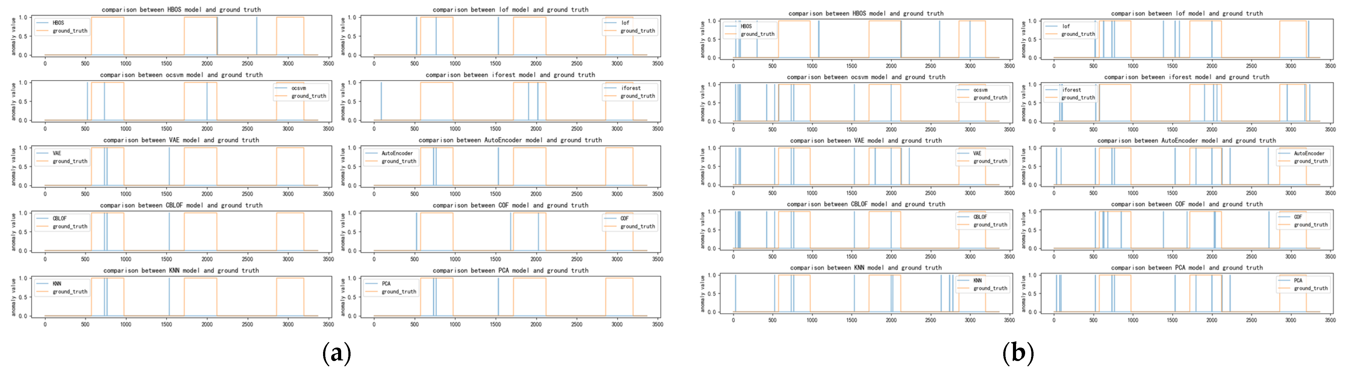
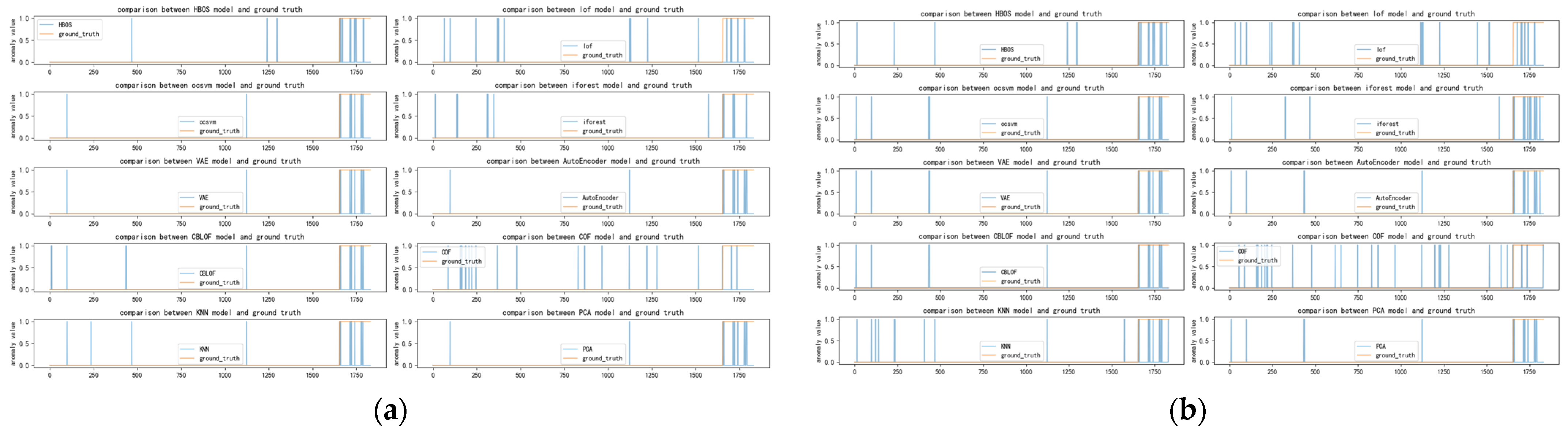
Figure A1.
(a) Distribution of anomalies with a time window of two for ad-cpc dataset; (b) Distribution of anomalies with a time window of ten for ad-cpc dataset.
Figure A1.
(a) Distribution of anomalies with a time window of two for ad-cpc dataset; (b) Distribution of anomalies with a time window of ten for ad-cpc dataset.
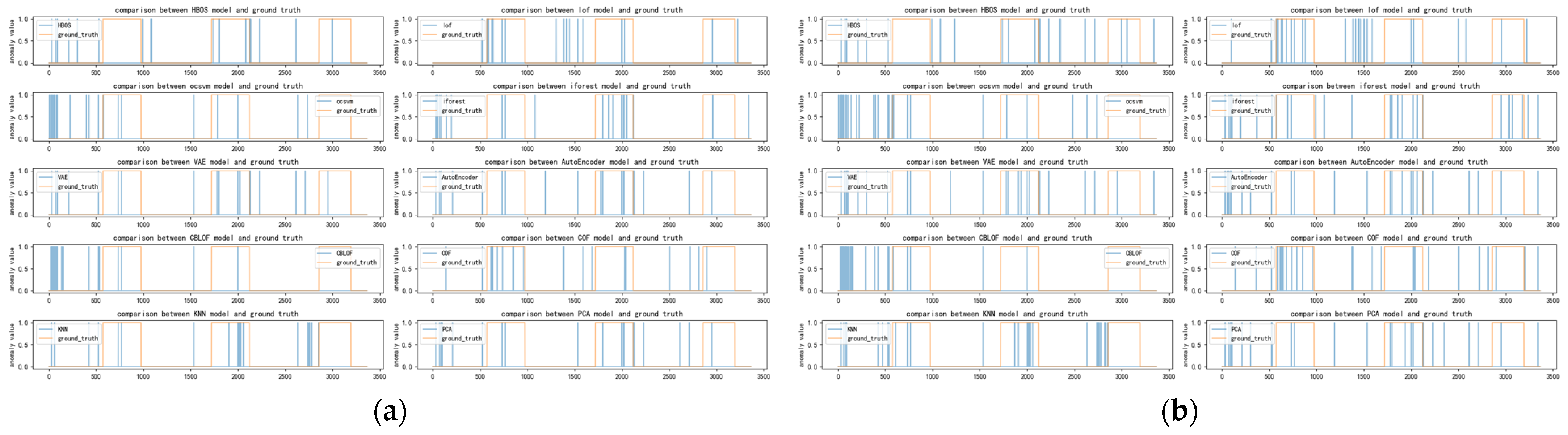
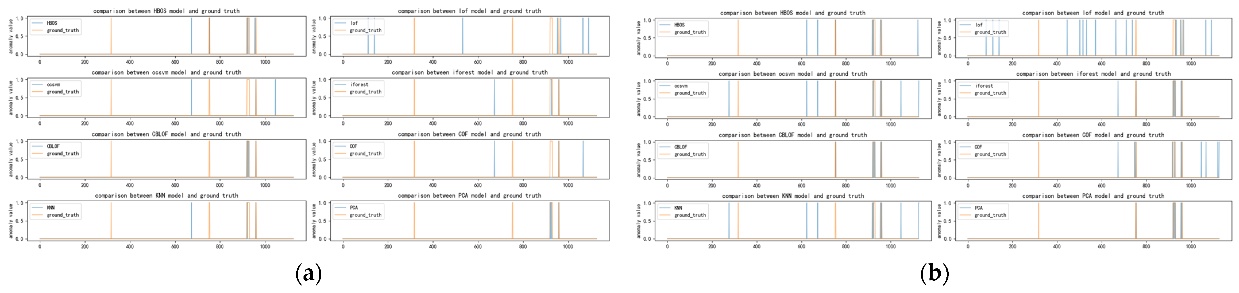
Figure A2.
(a) Distribution of anomalies with a time window of 20 for ad-cpc dataset; (b) Distribution of anomalies with a time window of 30 for ad-cpc dataset.
Figure A2.
(a) Distribution of anomalies with a time window of 20 for ad-cpc dataset; (b) Distribution of anomalies with a time window of 30 for ad-cpc dataset.
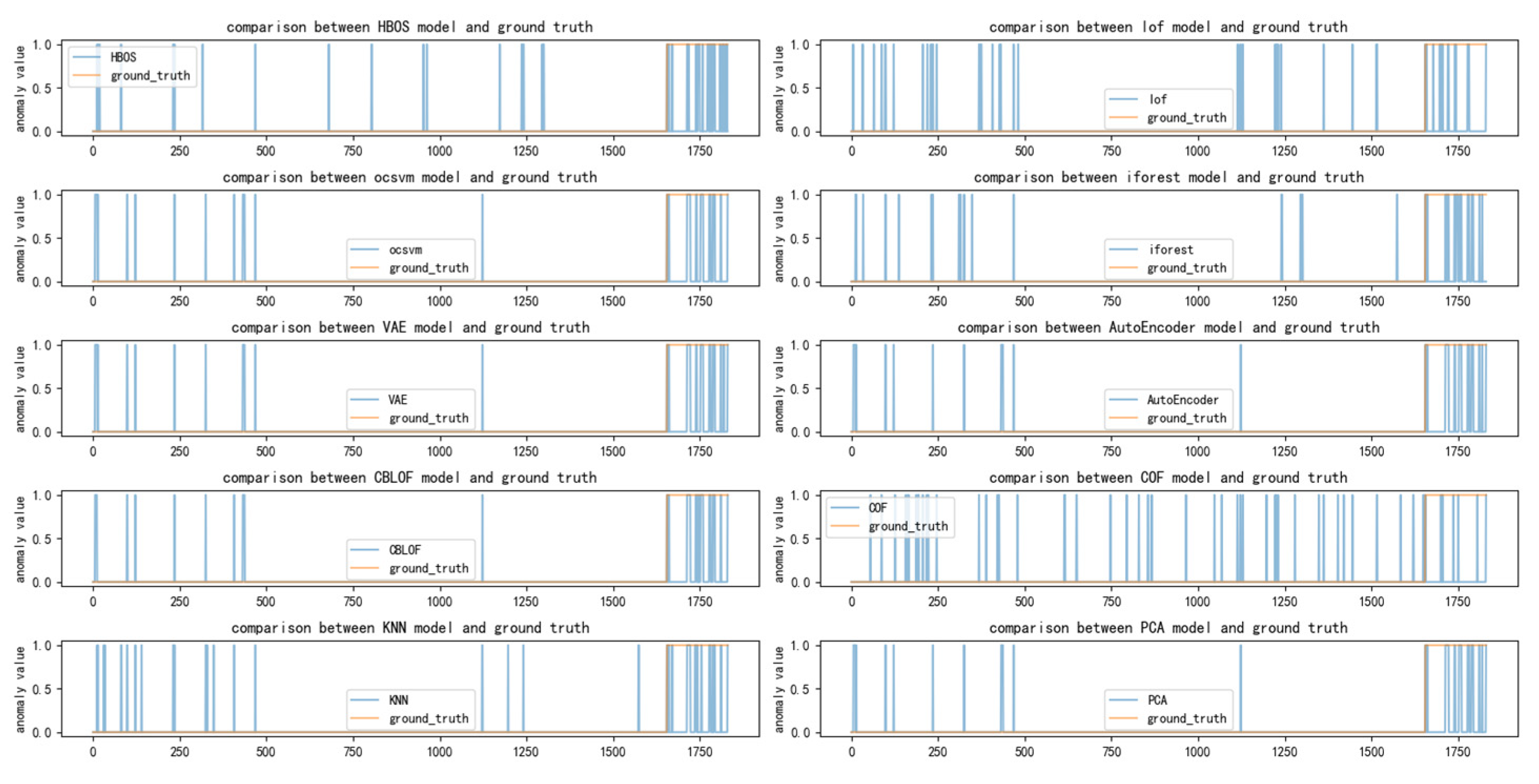
Figure A3.
(a) Distribution of anomalies with a time window of 40 for ad-cpc dataset; (b) Distribution of anomalies with a time window of 50 for ad-cpc dataset.
Figure A3.
(a) Distribution of anomalies with a time window of 40 for ad-cpc dataset; (b) Distribution of anomalies with a time window of 50 for ad-cpc dataset.
Figure A4.
Distribution of anomalies with a time window of 60 for ad-cpc dataset.
Figure A4.
Distribution of anomalies with a time window of 60 for ad-cpc dataset.
Table A1.
Algorithm selection result under different time windows for ad-cpc dataset.
Table A1.
Algorithm selection result under different time windows for ad-cpc dataset.
| Size of Time Windows | Detector of Choice | Time Widow Combination | Detector of Choice |
|---|
| 2 | LOF, COF | 2-10 | LOF, COF, |
| 10 | LOF, COF, | 2-20 | LOF, COF, |
| 20 | LOF, COF, IFOREST, KNN | 2-30 | LOF, COF |
| 30 | LOF, COF, KNN PCA | 2-40 | LOF, COF, KNN |
| 40 | LOF, COF, KNN | 2-50 | LOF, COF, KNN |
| 50 | LOF, COF, KNN | 2-60 | LOF, COF, KNN |
| 60 | LOF, COF, KNN | | |
The ap-cpc dataset exhibits similar characteristics to the occu dataset, featuring a higher number of anomalies, albeit with short durations. The eight base detectors applied to the speed dataset produce comparable detection results. With a small time window, each detector primarily identifies a single anomaly. As the time window expands, the number of correct detections of anomalies increases proportionally with the number of false detections. In contrast, our preferred method is less susceptible to variations in the time window, particularly when the time window is large, showing minimal changes. The experimental findings obtained from the ap-cpc dataset align with those of the occu dataset, reinforcing the consistency of the conclusions.
Figure A5,
Figure A6,
Figure A7 and
Figure A8 depict the classification of anomalous labels under different time windows in the speed dataset.
Table A2 presents the detectors selected by our algorithm with comparable performance under different time windows and the preferred detectors when combining multiple time windows.
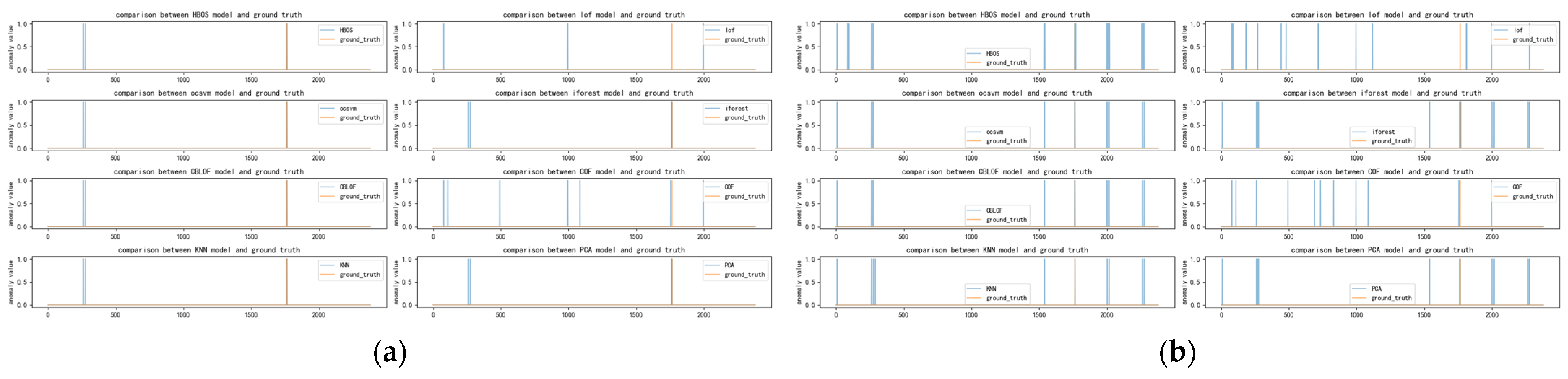
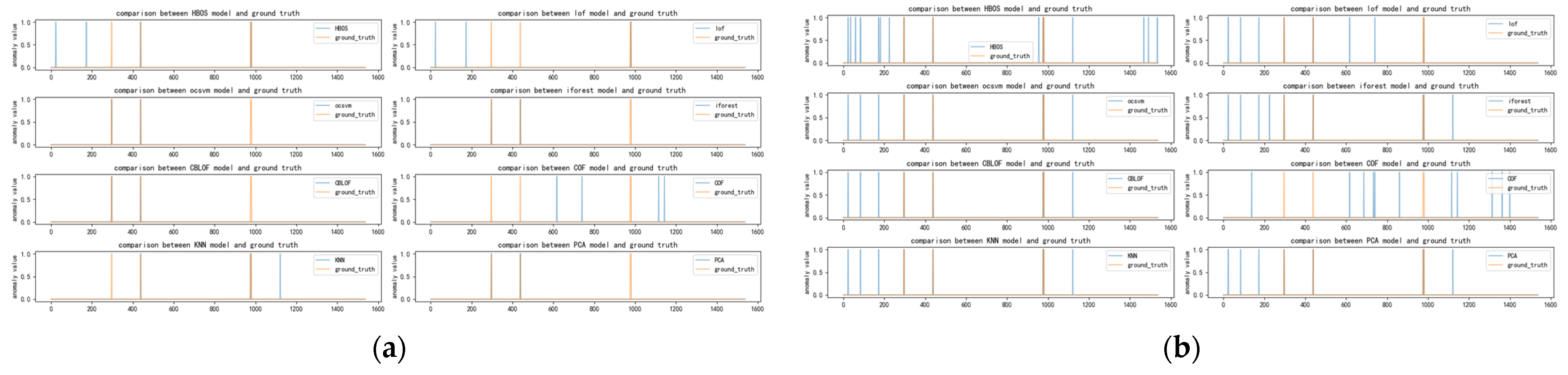
Figure A5.
(a) Distribution of anomalies with a time window of two for speed dataset; (b) Distribution of anomalies with a time window of ten for speed dataset.
Figure A5.
(a) Distribution of anomalies with a time window of two for speed dataset; (b) Distribution of anomalies with a time window of ten for speed dataset.
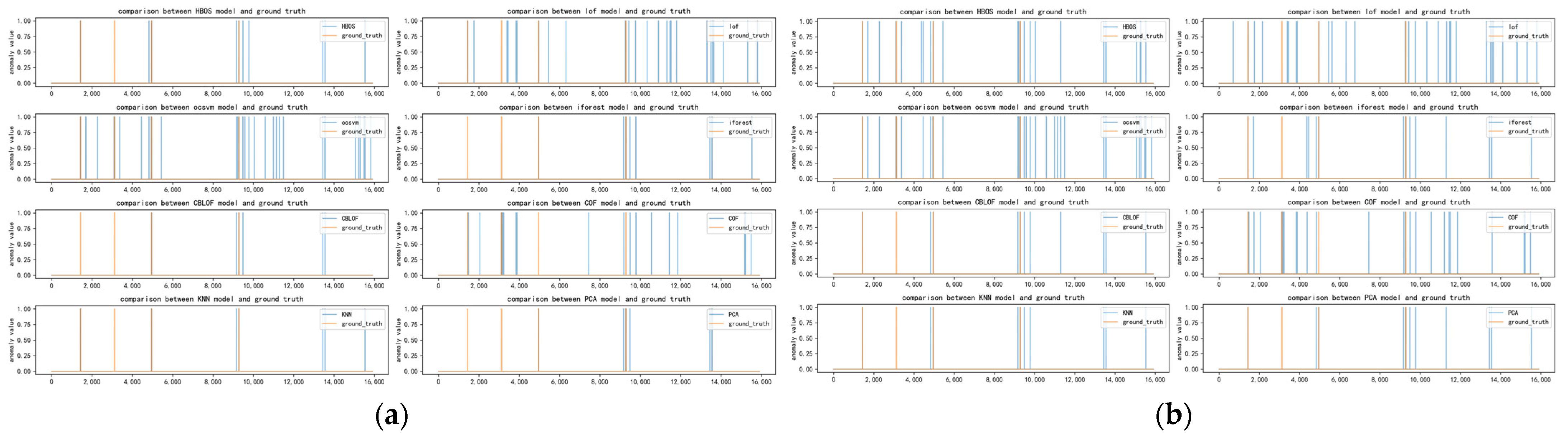
Figure A6.
(a) Distribution of anomalies with a time window of 20 for speed dataset; (b) Distribution of anomalies with a time window of 30 for speed dataset.
Figure A6.
(a) Distribution of anomalies with a time window of 20 for speed dataset; (b) Distribution of anomalies with a time window of 30 for speed dataset.
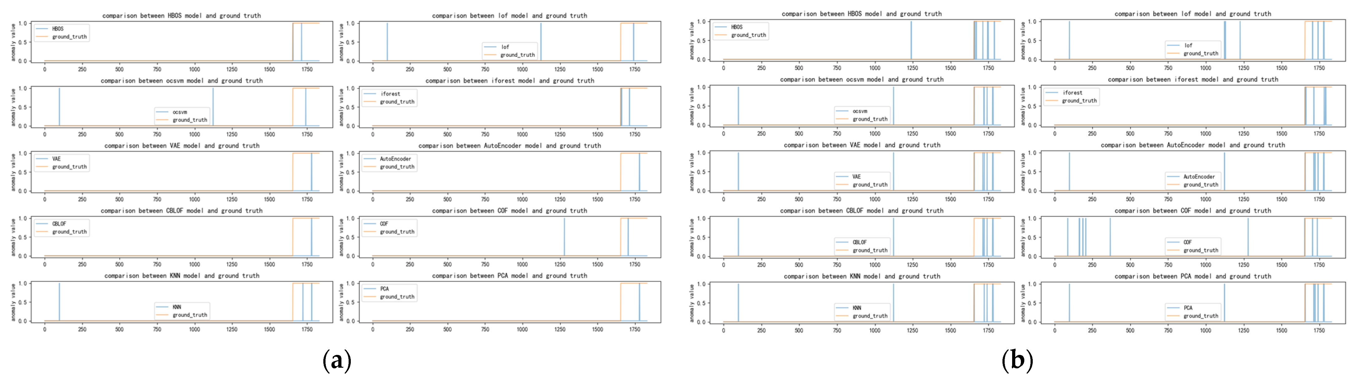
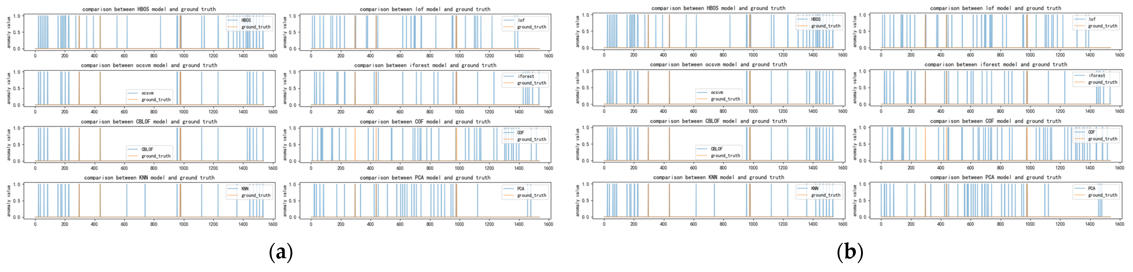
Figure A7.
(a) Distribution of anomalies with a time window of 40 for speed dataset; (b) Distribution of anomalies with a time window of 50 for speed dataset.
Figure A7.
(a) Distribution of anomalies with a time window of 40 for speed dataset; (b) Distribution of anomalies with a time window of 50 for speed dataset.
Figure A8.
Distribution of anomalies with a time window of 60 for speed dataset.
Figure A8.
Distribution of anomalies with a time window of 60 for speed dataset.
Table A2.
Algorithm selection result under different time windows for speed dataset.
Table A2.
Algorithm selection result under different time windows for speed dataset.
| Size of Time Windows | Detector of Choice | Time Widow Combination | Detector of Choice |
|---|
| 2 | HBOS, OCSVM, IFOREST, CBLOF, COF, KNN, PCA | 2-10 | HBOS, IFOREST, CBLOF, PCA |
| 10 | HBOS, IFOREST, CBLOF, PCA | 2-20 | HBOS, IFOREST, CBLOF, PCA |
| 20 | HBOS, IFOREST, CBLOF, PCA | 2-30 | HBOS, IFOREST, CBLOF, PCA |
| 30 | HBOS, IFOREST, CBLOF, PCA | 2-40 | HBOS, IFOREST, CBLOF, PCA |
| 40 | HBOS, IFOREST, CBLOF, KNN, PCA | 2-50 | HBOS, IFOREST, CBLOF, PCA |
| 50 | HBOS, IFOREST, CBLOF, KNN, PCA | 2-60 | HBOS, IFOREST, CBLOF, PCA |
| 60 | HBOS, OCSVM, IFOREST, CBLOF, KNN, PCA | | |
The experimental findings on the speed dataset exhibit remarkable similarities to the occu dataset. As depicted in
Table A2, it is evident that our selection method is not as effective on this particular dataset, despite successfully selecting the four detectors with the best performance.
Figure A9,
Figure A10,
Figure A11 and
Figure A12 depict the classification of anomalous labels under different time windows in the twitter dataset.
Table A3 presents the detectors selected by our algorithm with comparable performance under different time windows and the preferred detectors when combining multiple time windows.
Figure A9.
(a) Distribution of anomalies with a time window of two for twitter dataset; (b) Distribution of anomalies with a time window of ten for twitter dataset.
Figure A9.
(a) Distribution of anomalies with a time window of two for twitter dataset; (b) Distribution of anomalies with a time window of ten for twitter dataset.
Figure A10.
(a) Distribution of anomalies with a time window of 20 for twitter dataset; (b) Distribution of anomalies with a time window of 30 for twitter dataset.
Figure A10.
(a) Distribution of anomalies with a time window of 20 for twitter dataset; (b) Distribution of anomalies with a time window of 30 for twitter dataset.
Figure A11.
(a) Distribution of anomalies with a time window of 40 for twitter dataset; (b) Distribution of anomalies with a time window of 50 for twitter dataset.
Figure A11.
(a) Distribution of anomalies with a time window of 40 for twitter dataset; (b) Distribution of anomalies with a time window of 50 for twitter dataset.
Figure A12.
Distribution of anomalies with a time window of 60 for twitter dataset.
Figure A12.
Distribution of anomalies with a time window of 60 for twitter dataset.
Table A3.
Algorithm selection result under different time windows for twitter dataset.
Table A3.
Algorithm selection result under different time windows for twitter dataset.
| Size of Time Windows | Detector of Choice | Time Widow Combination | Detector of Choice |
|---|
| 2 | HBOS, OCSVM, IFOREST, CBLOF, KNN, PCA | 2-10 | HBOS, OCSVM, IFOREST, CBLOF, PCA |
| 10 | HBOS, OCSVM, IFOREST, CBLOF, PCA | 2-20 | HBOS, OCSVM, IFOREST, CBLOF, PCA |
| 20 | HBOS, OCSVM, IFOREST, CBLOF, PCA | 2-30 | HBOS, OCSVM, CBLOF |
| 30 | HBOS, OCSVM, CBLOF | 2-40 | HBOS, OCSVM, CBLOF |
| 40 | HBOS, OCSVM, CBLOF | 2-50 | HBOS, OCSVM, CBLOF |
| 50 | HBOS, OCSVM, CBLOF, KNN | 2-60 | HBOS, OCSVM, CBLOF |
| 60 | HBOS, OCSVM, CBLOF, KNN | | |
The twitter dataset, sourced from the NAB data source, exhibits anomaly characteristics that are essentially the same as those of the occu, speed, and other datasets, as depicted in
Figure A9,
Figure A10,
Figure A11 and
Figure A12. These figures clearly illustrate the anomaly detection results of each detector. Notably, OCSVM, LOF, and COF display prominent false alarm rates, while HBOS, CBLOF, IFOREST, and PCA exhibit more similar results. However, our method ultimately selects OCSVM, HBOS, and CBLOF, which may appear puzzling at first glance.
Upon closer inspection, it becomes evident that the twitter dataset contains a significantly larger amount of data compared to the other datasets. Although it might seem that OCSVM should have more overlap with LOF, COF, and other detectors based on the graphs, in reality, the overlap is not as substantial as it appears, possibly due to the effects of shrinkage. The concentration of true anomalies emerges as the crucial factor in selecting an anomaly detector. However, this concentration is also a side effect of using a large time window for discrete anomalies.
Figure A13,
Figure A14,
Figure A15 and
Figure A16 depict the classification of anomalous labels under different time windows in the vowels dataset.
Table A4 presents the detectors selected by our algorithm with comparable performance under different time windows and the preferred detectors when combining multiple time windows.
Figure A13.
(a) Distribution of anomalies with a time window of two for vowels dataset; (b) Distribution of anomalies with a time window of ten for vowels dataset.
Figure A13.
(a) Distribution of anomalies with a time window of two for vowels dataset; (b) Distribution of anomalies with a time window of ten for vowels dataset.
Figure A14.
(a) Distribution of anomalies with a time window of 20 for twitter dataset; (b) Distribution of anomalies with a time window of 30 for vowels dataset.
Figure A14.
(a) Distribution of anomalies with a time window of 20 for twitter dataset; (b) Distribution of anomalies with a time window of 30 for vowels dataset.
Figure A15.
(a) Distribution of anomalies with a time window of 40 for vowels dataset; (b) Distribution of anomalies with a time window of 50 for vowels dataset.
Figure A15.
(a) Distribution of anomalies with a time window of 40 for vowels dataset; (b) Distribution of anomalies with a time window of 50 for vowels dataset.
Figure A16.
Distribution of anomalies with a time window of 60 for vowels dataset.
Figure A16.
Distribution of anomalies with a time window of 60 for vowels dataset.
Table A4.
Algorithm selection result under different time windows for vowels dataset.
Table A4.
Algorithm selection result under different time windows for vowels dataset.
| Size of Time Windows | Detector of Choice | Time Widow Combination | Detector of Choice |
|---|
| 2 | LOF, IFOREST, KNN | 2-10 | IFOREST, KNN |
| 10 | IFOREST, CBLOF, KNN | 2-20 | LOF, IFOREST, CBLOF, KNN |
| 20 | LOF, OCSVM, CBLOF, COF, KNN | 2-30 | LOF, CBLOF, KNN |
| 30 | LOF, CBLOF, KNN | 2-40 | LOF, CBLOF, COF, KNN |
| 40 | LOF, CBLOF, COF, KNN | 2-50 | LOF, CBLOF, KNN |
| 50 | LOF, CBLOF, KNN | 2-60 | LOF, CBLOF, KNN |
| 60 | LOF, OCSVM, CBLOF, COF, KNN | | |
The vowels dataset is a multidimensional dataset that shares similarities with the cardio dataset. As the time window increases, the figures indicate that the results of each detector begin to concentrate in different regions. Detectors with scattered anomaly results are eliminated, while those exhibiting concentration in a particular region, regardless of correct or incorrect anomalies, are selected. The different time windows also influence the final detector selection. Although the selection results tend to stabilize with LOF, CBLOF, and KNN, there are occasional instances where other detectors are chosen. It is evident that our method is not yet fully stable on this dataset, as observed from the fluctuating selection outcomes.


