Breaking the ImageNet Pretraining Paradigm: A General Framework for Training Using Only Remote Sensing Scene Images

Abstract

Remote sensing scene classification (RSSC) is a very crucial subtask of remote sensing image understanding. With the rapid development of convolutional neural networks (CNNs) in the field of natural images, great progress has been made in RSSC. Compared with natural images, labeled remote sensing images are more difficult to acquire, and typical RSSC datasets are consequently smaller than natural image datasets. Due to the small scale of these labeled datasets, training a network using only remote sensing scene datasets is very difficult. Most current approaches rely on a paradigm consisting of ImageNet pretraining followed by model fine-tuning on RSSC datasets. However, there are considerable dissimilarities between remote sensing images and natural images, and as a result, the current paradigm may present some problems for new studies. In this paper, to break free of this paradigm, we propose a general framework for scene classification (GFSC) that can help to train various network architectures on limited labeled remote sensing scene images. Extensive experiments show that ImageNet pretraining is not only unnecessary but may be one of the causes of the limited performance of RSSC models. Our study provides a solution that not only replaces the ImageNet pretraining paradigm but also further improves the baseline for RSSC. Our proposed framework can help various CNNs achieve state-of-the-art performance using only remote sensing images and endow the trained models with a stronger ability to extract discriminative features from complex remote sensing images.

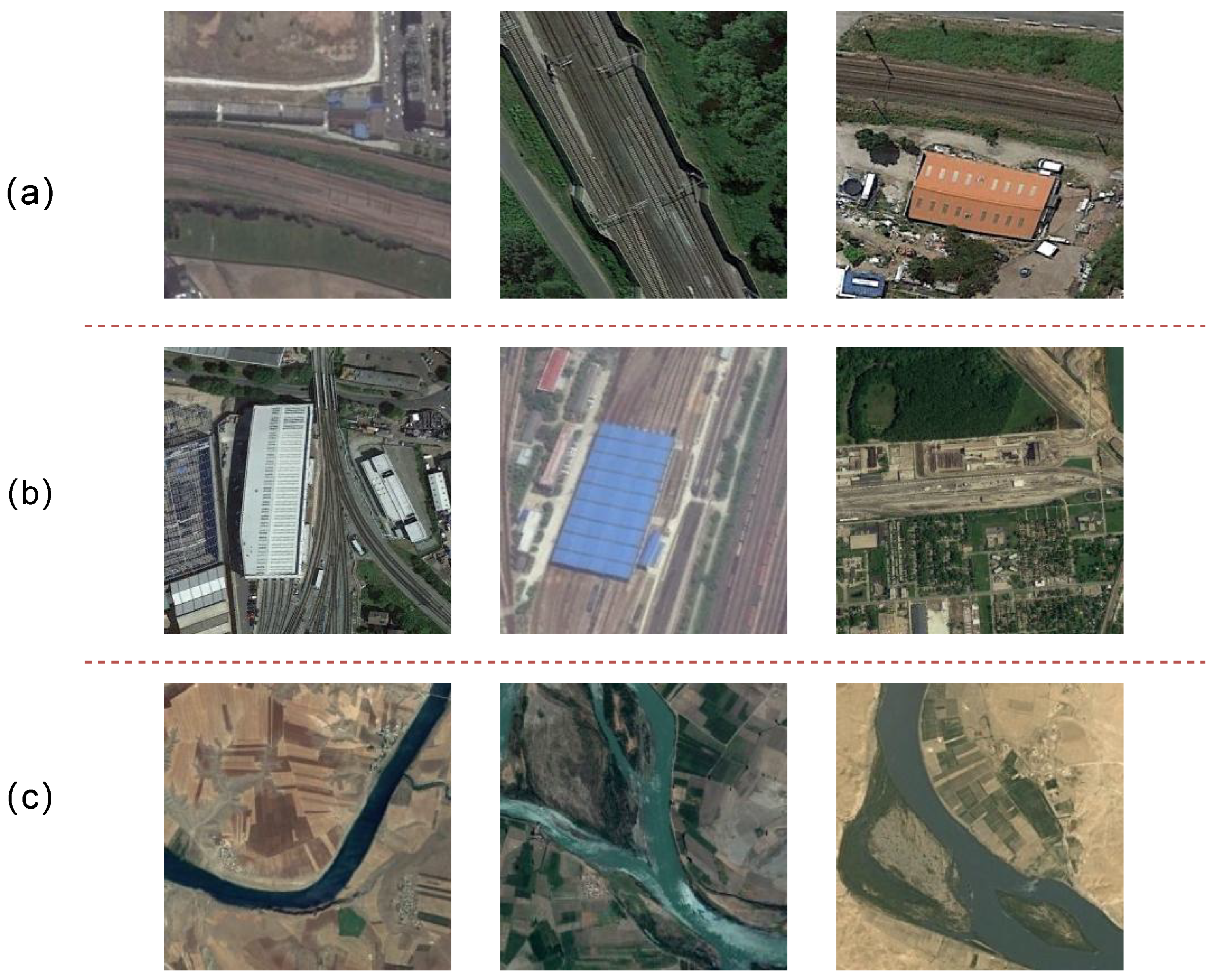
1. Introduction

The goal of remote sensing scene classification (RSSC) is to classify each patch segmented from remote sensing images to a meaningful land cover type [1,2,3,4,5]. RSSC can play a critical role in tasks such as urban planning [6] and pollution detection [7], as well as many downstream tasks such as change detection [8] and remote sensing image segmentation and object detection [9,10]. Although much progress has been achieved in RSSC, it is still a very challenging task. As shown in Figure 1, remote sensing scenes include large variations in object/scene scales and the coexistence of multiple ground objects [11]. Furthermore, remote sensing scenes exhibit high intraclass diversity and interclass similarity.

Many convolutional neural network (CNN)-based methods have been proposed to improve the classification accuracy of RSSC [12,13,14,15]. By virtue of the enormous data volumes of natural image datasets and the representation capabilities of CNNs, RSSC performance has been continuously improved. Cheng et al. [16] proposed discriminative CNNs (DCNNs) to boost performance on RSSC tasks. Lu et al. [17] proposed a feature aggregation CNN (FACNN) to learn scene representations directly from remote sensing scene datasets. Based on feature fusion, Xue et al. [18] proposed the multi-structure deep feature fusion (MSDFF) framework. However, although many CNN-based methods have achieved good performance for RSSC, the related studies have mostly followed a paradigm consisting of ImageNet pretraining followed by model fine-tuning on RSSC datasets. To the best of our knowledge, there are still relatively few studies that have focused on improving classification accuracy using only remote sensing images without ImageNet pretraining. However, this topic is critical for further development in this domain.

As shown in Figure 1, there are significant differences between remote sensing images and natural images in terms of image intensity values, wavebands, resolutions, object scales, etc. As shown in

Table 1. Comparison of RSSC datasets and natural image datasets.

Dataset	Classes	Total Images	Images/Class
Natural Image Datasets:
ImageNet (2012) [19]	1000	1,431,167	∼1000
MNIST [20]	10	60,000	6000
CIFAR-10 [21]	10	60,000	6000
RSSC Datasets:
NWPU-RESISC45 [22]	45	31,500	700
AID [23]	30	10,000	200–420
PatternNet [24]	38	30,400	800
UC-Merced [25]	21	2100	100

, the available labeled remote sensing image datasets contain much fewer images than natural image datasets. Therefore, if a model is trained using only remote sensing images, a degradation in accuracy will result due to the relative lack of data, as demonstrated in Figure 2. This gap in performance with and without ImageNet pretraining may lead to the following problems: (1) most of the widely used models are pretrained on ImageNet, but some models are not open-access, such as ResNet-9 and WRN-9, as well as some self-defined models; (2) when the network structure is modified or a new network structure is designed, pretraining on ImageNet is required to achieve good results, but such pretraining requires many GPU hours; (3) since fine-tuning does not change the weights significantly, the feature extraction performance is partially limited by the features learned from ImageNet and cannot be specifically adapted to remote sensing images; and (4) the quality of the pretrained model has a significant impact on the results, especially as the number of available training techniques and new structures increases, making it difficult to evaluate multiple different networks for the same task. These issues lead us to consider the following questions: Is ImageNet pretraining necessary? Can we train CNNs using only remote sensing images?

Researchers have long been accustomed to improving performance based on backbone networks pretrained on ImageNet, but ImageNet pretraining may, in fact, limit the performance of methods based on it. To explore possible solutions to address the decrease in accuracy caused by model training without ImageNet pretraining, we propose a general framework to help train various CNNs using only remote sensing images. Accordingly, we answer the previous questions as follows: ImageNet pretraining is not necessary, and state-of-the-art results can be achieved using only remote sensing images. The proposed framework comprises three steps, as shown in Figure 3: (1) self-supervised learning for weight initialization, (2) learning specific data augmentation strategies, and (3) training under regularization strategy. Our experiments suggest that our proposed general framework for RSSC (GFSC) allows CNNs to achieve comparable state-of-the-art results when trained only on RSSC datasets. At the same time, the models trained under GFSC can extract more discriminative features than the models using ImageNet pretraining. We note that almost all individual components of our framework have appeared in previous work, although their specific implementations may be different. The superiority of our framework relative to previous work is not explained by any single design choice, but rather by their combination. The main contributions of this paper are as follows:

• We propose a general training framework, GFSC, for training RSSC models without ImageNet pretraining. This framework can achieve results that surpass those of methods based on ImageNet pretraining using only remote sensing images.
• Compared with ImageNet pretraining, GFSC enables the extraction of more discriminative features with less consumption of computational resources.
• Our proposed framework is easy to implement, exhibits good generalizability to different CNN structures, and yields consistent performance improvements.

The rest of this paper is organized as follows. Section 2 reviews the related work of this paper. Then, the proposed GFSC is introduced in Section 3. Experiments conducted to test the proposed method are described in Section 4. Finally, we conclude this article in Section 5.

2. Related Work

In this section, we give a brief review of existing related works on the development of CNN architectures, transfer learning in RSSC, and self-supervised learning of image representations.

2.1. Modern CNN Architectures

Since the emergence of ImageNet [26] and AlexNet [27], CNN-based methods have undergone rapid development. In particular, CNN-based methods have dominated research on image classification and many downstream tasks. GoogLeNet [28] adopts $1\times 1$ convolutional layers to learn nonlinear combinations of the feature map channels and uses a global average pooling (GAP) layer in the place of heavy fully connected layers. By repeatedly stacking $3\times 3$ small convolutional kernels, VGG-Net [19] built very deep networks. Building on the success of these pioneering studies, the authors of ResNet [29] introduced the design of residual learning to ease the degradation problem in stacking more layers and empower networks to increase depth. To improve the performance, a wide residual network (WRN) [30] is proposed as a novel architecture to increase the width of residual networks. Xie et al. [31] proposed the ResNeXt architecture based on aggregated residual transformations. These network architectures are widely used as backbone networks for RSSC tasks.

2.2. Transfer Learning in RSSC

The purpose of transfer learning is to leverage knowledge from the source domain to boost the learning ability in the target domain [32,33,34]. Pretrained models on large-scale datasets have been reported to have better generality than randomly initialized models. Fine-tuning [35,36] is one powerful method for transfer learning. For RSSC tasks, the majority of state-of-the-art approaches rely on a paradigm consisting of pretraining on ImageNet and then fine-tuning on the target dataset. The marginal center loss [37] was proposed to overcome the challenges presented by large intraclass variations. Liu et al. [38] proposed a Siamese CNN that combines identification and verification models based on CNNs. A multisource compensation network (MSCN) [39] has been proposed to address the problems of distribution discrepancy and category incompleteness by using pretrained CNNs. Based on bilinear pooling [40] and hierarchical attention [41], Yu et al. [5] presented a feature fusion framework for RSSC. Most of these advanced approaches do not use the CNN backbone directly but build on it with a lot of careful design.

2.3. Self-Supervised Learning of Image Representations

Self-supervised learning (SSL) is a new paradigm that focuses on designing pretext tasks to learn a good representation [42,43]. SSL learns directly from unlabeled data and does not require labeled data. This will eliminate the requirement for large amounts of labeled data, which can be expensive to acquire. Many training approaches have been proposed for learning image representations via SSL. Chen et al. [44] proposed SimCLR, which is a simple contrastive learning framework for visual representations. He et al. [45] proposed Momentum Contrast (MoCo) for SSL with a contrastive loss. Bootstrap Your Own Latent (BYOL) [46] is designed to use only positive pairs and achieves state-of-the-art results under the linear evaluation protocol on ImageNet.

3. Proposed Method

3.1. Overview of the Proposed Framework

Learning good feature representations from limited data is a very challenging task. To address this challenge, we attempt to make full use of the original data. As mentioned previously, remote sensing images are different from natural images in many respects, so it is important to design specific methods consistent with the characteristics of remote sensing images. Indeed, some methods designed for application to natural images can even compromise the performance on RSSC tasks if they are used inappropriately. To this end, the end-to-end GFSC is proposed to help train CNNs on limited data. Figure 3 illustrates the core idea of our proposed framework, GFSC. The goal of our method is to help various backbones achieve results comparable to those of models with ImageNet pretraining using only RSSC datasets.

As shown in Figure 3, Starting from the overall training process, we consider various elements of the process to address the degradation of RSSC model training without ImageNet pretraining. For the initialization of the weights, we employ SSL to learn the characteristics of the remote sensing images themselves. Data augmentation and regularization strategies are also important when the amount of data is insufficient. For data augmentation, we learn suitable data augmentation strategies specific to RSSC datasets. For regularization, we use Mixup as the regularization strategy.

3.2. SSL for Weight Initialization

Recently, SSL has received considerable attention and has enabled much progress in the field of natural images. Inspired by these studies, we use BYOL for the initialization of the weights.

BYOL is a new algorithm for the SSL of image representations [46]. Its target is to learn a good representation $y_{\theta }$ that can then be used for other downstream tasks. This algorithm is composed of two networks: an online network and a target network. The two networks interact with and learn from each other.

The online network is defined by a set of weights $\theta$ and is composed of three stages: an encoder $y_{\theta }$, a projector $g_{\theta }$, and a predictor $q_{\theta }$. The target network is similarly defined by a set of weights $\xi$ but is composed of only two stages: an encoder $y_{\xi }$ and a projector $g_{\xi }$.

As shown in Figure 4, the target network provides the regression targets to train the online network, and its parameters $\xi$ are exponential moving averages of the online parameters $\theta$. It achieves this goal by minimizing the L2 loss between the two representations $\overline{q_{\theta }}\left(z_{\theta }\right)$ and ${\overline{z}}_{\xi }^{\prime }$. During backpropagation, the target network is subjected to a stop-gradient operation. More specifically, after each training step, the following update is performed:

$$\xi \leftarrow m\xi +(1-m)\theta$$

(1)

where m is a target decay rate such that $m\in [0,1]$, $\theta$ represents online parameters, and $\xi$ are exponential moving averages of the online parameters $\theta$.

Let image x be sampled uniformly from a set of images D, and let $\mathcal{T}$ and ${\mathcal{T}}^{\prime }$ be two distributions of image augmentations. First, by applying image augmentations $t\sim \mathcal{T}$ and $t^{\prime }\sim {\mathcal{T}}^{\prime }$, we can obtain two augmented views v and $v^{\prime }$, respectively. Next, the online network outputs a representation $y_{\theta }$ and a projection $z_{\theta }$ from the first augmented view v, and the target network outputs the target representation $y_{\xi }^{\prime }$ and the target projection $z_{\xi }^{\prime }$ from the second augmented view $v^{\prime }$. Then, we can obtain two representations $q_{\theta }\left(z_{\theta }\right)$ and $z_{\xi }^{\prime }$. Since we need to compute the distance between these two representations, L2 normalization is applied to both $q_{\theta }\left(z_{\theta }\right)$ and $z_{ϵ}^{\prime }$. After L2 normalization, we obtain the two corresponding representations $\overline{q_{\theta }}\left(z_{\theta }\right)$ and ${\overline{z}}_{\xi }^{\prime }$.

The goal of our network is to push the prediction of the online network, $\overline{q_{\theta }}\left(z_{\theta }\right)$, closer to the target network’s projection, ${\overline{z}}_{\xi }^{\prime }$. Thus, the loss function can be defined as follows:

$$L_{\theta ,\xi }\triangleq {\parallel \overline{q_{\theta }}\left(z_{\theta }\right)-{\overline{z}}_{\xi }^{\prime }\parallel }_2^2=2-2·\frac{\langle q_{\theta }\left(z_{\theta }\right),z_{\xi }^{\prime }\rangle }{\parallel q_{\theta }\left(z_{\theta }\right){\parallel }_2·{\parallel z_{\xi }^{\prime }\parallel }_2}$$

(2)

where $\theta$ and $\xi$ denote the parameters of the online and target networks, respectively, $z_{\theta }$ represents the input data, and $L_{\theta ,\xi }$ denotes the loss function.

During the training phase, we can also feed $v^{\prime }$ into the online network and v into the target network to make fuller use of the data, and this loss can be symmetrized, yielding ${\tilde{L}}_{\theta ,\xi }$. In each step of training, we perform stochastic optimization to minimize $L_{\theta ,\xi }^{Total}=L_{\theta ,\xi }+{\tilde{\mathcal{L}}}_{\theta ,\xi }$ with respect to the online network $\theta$ only. It should be noted that the target network $\xi$ is subjected to a stop-gradient operation to prevent network collapse, and we retain only the encoder $f_{\theta }$.

3.3. Learning Specific Data Augmentation Strategies

Data augmentation is an important technique to improve the generalization ability of CNN models, and this technique is especially important in the case of insufficient labeled remote sensing images. Due to the differences between natural images and remote sensing images, it is important to learn data augmentation strategies that are specific to remote sensing images. However, in the absence of sufficient annotated remote sensing images, related data augmentation techniques have received relatively little attention. Considering the GPU hours consumed by searching for candidate policies, in this paper, we adopt an algorithm called Fast AutoAugment (FAA) [47] that can find effective augmentation policies via a relatively efficient search strategy based on density matching.

The whole process is illustrated in Figure 5. First, the training dataset $D_{train}$ is split into K folds, each of which consists of two datasets, $D_M^{\left(k\right)}$ and $D_A^{\left(k\right)}$. For each fold, we train a model based on $D_M^{\left(k\right)}$ and obtain the model parameters ${\theta }^k$. After the parameters ${\theta }^k$ are trained, B bundles of augmentation policies are sampled from sets of predefined data augmentation operators. Then, based on the evaluation results for model ${\theta }^k$, the top N policies in B are selected to obtain $T_{*}^{\left(K\right)}$ on $D_A^{\left(k\right)}$. Finally, the top N policies $T_{*}^{\left(K\right)}$ obtained from each of the K folds are appended to an augmentation list $T_{*}$.

Unlike previous methods such as AutoAugment [48], FAA does not train the model parameters $\theta$ many times, so it can find data augmentation strategies that are suitable for RSSC datasets in less time.

3.4. Mixup Strategy for Regularization

The diversity of the training samples is directly influenced to the generalization power of deep convolutional neural networks [49]. Many studies have demonstrated that constructing virtual samples can effectively improve the generalization ability of deep convolutional networks and prevent network overfitting [50,51].

However, due to the gap between natural images and remote sensing images, a regularization strategy that works on natural images may not be suitable for remote sensing images. Based on preliminary experiments, Mixup [52] is adopted as the regularization strategy in this paper.

Mixup is used in the training phase and not in the testing phase. In each iteration of training phase, we randomly select two samples, $(x_i,y_i)$ and $(x_j,y_j)$. Then, we form a new sample by performing weighted linear interpolation of these two samples:

$$\begin{array}{c}\widehat{x}=\lambda x_i+(1-\lambda )x_j\hfill \\ \widehat{y}=\lambda y_i+(1-\lambda )y_j\hfill \end{array}$$

(3)

where $\lambda$ is a random number in $[0,1]$. $\lambda$ is sampled from the $Beta(\alpha ,\alpha )$ distribution. This manner brings more randomness and makes the model more robust to such generated samples. In Mixup training phrase, we use only the new sample $(\widehat{x},\widehat{y})$.

In each iteration of training phase, a mixed sample $(\widehat{x},\widehat{y})$ is generated by combining two randomly selected training samples in a mini-batch. This strategy can be utilized to efficiently train any network architecture.

In addition to Mixup, we have also tested patch-based regularization strategies, such as CutMix [53]. Compared with objects in natural images, objects in remote sensing images often exist against more complex backgrounds. Consequently, patch-based methods often fail to construct meaningful samples and can even cause the accuracy to degrade.

4. Experiments

In this section, the proposed GFSC is performed on different representative RSSC datasets for evaluation. First, the experimental settings are described in Section 4.1. Second, the effectiveness of SSL is investigated in Section 4.2. Third, several ablation experiments are reported in Section 4.3. Fourth, GFSC is compared with other state-of-the-art methods in Section 4.4. Finally, visualizations are presented, and the effectiveness of the method is analyzed.

4.1. Experimental Settings

4.1.1. Datasets

In this paper, we report experiments conducted on several datasets widely used in RSSC. The details of these datasets can be found in Table 1.

The NWPU-RESISC45 dataset [22] is a publicly available benchmark dataset for RSSC task. It contains 45 types of remote sensing scene images with an overall size of 31,500. Each scene class of this dataset contains 700 images with $256\times 256$ pixels. The common training ratio of this dataset is 10% and 20%. The Aerial Image Dataset (AID) dataset [23] contains 10,000 scene images divided into 30 remote sensing scene classes. Each scene class of the AID dataset contains 200 to 400 images with $600\times 600$ pixels. The common training ratio of this dataset is 20% and 50%.

The UC-Merced dataset [25] contains 2100 scene images divided into 21 land-use classes. Each scene class of this dataset contains 100 images with $256\times 256$ pixels. The common training ratio of this dataset is 50% and 80%.

PatternNet [24] is a large-scale benchmark dataset for remote sensing image retrieval. Different from above datasets, PatternNet is designed specially for the task of remote sensing image retrieval. The images of this dataset were collected from Google Earth imagery or via the Google Maps API for US cities. It contains 38 remote sensing scenes. Each scene class of this dataset contains 800 images with $256\times 256$ pixels.

The NAP (NWPU-RESISC45+AID+PatternNet) dataset is an unlabeled dataset for self-supervised pretraining. It is a combination of the AID, NWPU, and PatternNet datasets. The total number of images in this dataset is 71,900.

The NAP+ dataset is a large-scale unlabeled remote sensing image dataset built on top of the NAP dataset. Since unlabeled data are easier to collect than labeled data, we collected numerous unlabeled remote sensing images from the Google Maps API with the aim of exploring the boundaries of SSL. The total number of images is 200,000 in this dataset.

4.1.2. Implementation Details

All models in the experiments were implemented using the deep learning framework PyTorch. The experiments were performed on a workstation with 32 GB of memory and two 2.6 GHz ten-core CPUs. Two NVIDIA RTX Titan GPUs with 24 GB memory were used for acceleration. In the phase of SSL for pretraining, the images were randomly cropped to a size of $96\times 96$ pixels, the learning rate was 0.6, and the optimizer was LARS [54]. In the fine-tuning stage, the images were resized to $256\times 256$ pixels. Stochastic gradient descent (SGD) was used as optimization method. The learning rates for ImageNet pretraining and SSL-based pretraining were 0.001 and 0.01, respectively. The learning rates were first warmed up for 5 epochs, followed by a cosine leaning rate decay in the rest of epochs [55]. All networks were trained for 100 epochs in order to ensure fair comparisons. In order to have a better convergence of the CNNs, we only used Mixup for the first 80 epochs. To obtain reliable results, we performed each experiment 5 times. The means and standard deviations of the five experiments are reported.

4.2. Effectiveness of SSL

Well-labeled remote sensing data are very expensive to acquire, but unlabeled remote sensing scene images are easy to obtain. Using SSL for model initialization is one of the keys to the success of our proposed framework. In this section, to verify the effectiveness of SSL as a model initialization strategy, we report experiments conducted on several representative backbone networks, including ResNet, ResNeXt, and WRN. The models were pretrained on the ImageNet dataset for 120 epochs and on the NAP and NAP+ datasets using SSL for 300 epochs. To ensure fair comparisons, all methods were fine-tuned on the NWPU dataset for 100 epochs using the default data augmentation strategy on ImageNet. It is important to note that other components of GFSC are not used at this stage.

4.2.1. Influence of the Cropped Image Size on SSL

In SSL, the size to which the images are cropped is an important factor affecting the time and computational effort of training. Because of the large dissimilarities between remote sensing images and natural images, to explore the effects of different image resolutions on the characterization ability of the network, we compare the top-1 accuracies achieved under different random crop sizes in Figure 6. From the results in this figure, it is obvious that SSL is not highly sensitive to the crop size for remote sensing images. If the crop size is increased, it will bring more GPU hours and memory usage. Considering training time and resource consumption, we adopted a crop size of 96 in the subsequent SSL experiments.

4.2.2. Comparison with Random Initialization

We performed experiments on three representative backbone networks and found that using SSL for network initialization yielded significant improvements compared to random initialization. We needed only a very small number of GPU hours for initialization to obtain much better results than those achieved with random initialization. The consistent performance gains obtained on the three backbone networks indicate that our proposed framework is effective for different network designs, reflecting the robustness of our approach to some extent.

4.2.3. Comparison with ImageNet Pretraining

ImageNet is a very large dataset that requires not only a large storage space but also a very large number of GPU hours to initialize a model on it, and in general, it is difficult to train models on this dataset. As shown in

Table 2. Comparisons of random initialization, ImageNet pretraining, and SSL, where T.R. is an abbreviation for training ratio.

Method	Param (M)	Pretraining Details				NWPU-RESISC45
		Total Images	Storage (GB)	Epochs	Pretraining GPU Hours	T.R. = 10%	T.R. = 20%
Random Initialization:
ResNet-50	23.60	—	—	—	—	$65.89\pm 1.25$	$81.44\pm 0.24$
ResNeXt-50	23.07	—	—	—	—	$72.10\pm 0.64$	$82.26\pm 0.28$
WRN-50	66.93	—	—	—	—	$65.78\pm 0.41$	$81.82\pm 0.58$
ImageNet Pretraining:
ResNet-50	23.60	1,431,167	155.38	120	227.52	$89.99\pm 0.11$	$92.95\pm 0.19$
ResNeXt-50	23.07	1,431,167	155.38	120	270.76	$91.04\pm 0.19$	$93.59\pm 0.13$
WRN-50	66.93	1,431,167	155.38	120	338.86	$90.52\pm 0.24$	$93.53\pm 0.18$
SSL on NAP:
ResNet-50	23.60	71,900	4.59	300	4.15	$89.58\pm 0.25$	$92.21\pm 0.12$
ResNeXt-50	23.07	71,900	4.59	300	5.92	$89.98\pm 0.13$	$92.96\pm 0.12$
WRN-50	66.93	71,900	4.59	300	6.19	$90.70\pm 0.15$	$93.41\pm 0.19$
SSL on NAP+:
ResNet-50	23.60	200,000	17.81	300	10.55	$91.55\pm 0.12$	$93.79\pm 0.16$
ResNeXt-50	23.07	200,000	17.81	300	14.55	$92.70\pm 0.19$	$94.48\pm 0.12$
WRN-50	66.93	200,000	17.81	300	14.61	$92.80\pm 0.17$	$94.55\pm 0.13$

, compared to ImageNet pretraining, our framework needs a much smaller amount of storage space and much fewer GPU hours for training to obtain comparable results on the NAP dataset. With SSL on such limited remote sensing images as pretraining, WRN-50 obtains even better results than those achieved with ImageNet pretraining.

4.2.4. Beyond ImageNet Pretraining

Intuitively, training on more data can improve the representational and generalization capabilities of a model. To explore the boundaries of our proposed method, we also conducted experiments on a larger dataset, NAP+. One exciting finding is that we can obtain better results than with ImageNet pretraining while incurring much less consumption of computational resources. Without any modifications to the network, self-supervised training on the NAP+ dataset followed by fine-tuning on the NWPU dataset yields better results than ImageNet pretraining. Taking the ResNet-50, ResNeXt-50, and WRN-50 networks as examples, we achieved improvements of 0.84%, 0.89%, and 1.02%, respectively, compared with ImageNet pretraining at a 20% training ratio on the NWPU dataset. These experimental results reflect that better representations can be learned by using only remote sensing images. The CNN backbones learned in this manner are more specific for the remote sensing images.

4.3. Ablation Study

In addition to the method of weight initialization, two major improvements are introduced in the framework proposed in this paper to help train models on limited remote sensing images: the specific data augmentation strategy search and the regularization strategy. In this section, we explore the effectiveness of these two improvements. We investigated each component of GFSC by designing several controlled experiments on NWPU-RESISC45. For convenient performance comparisons, ResNet-50 initialized via SSL on NAP+ was used to explore the performance of the different components.

4.3.1. Data Augmentation in GFSC

We analyzed the effect of the search for data augmentation strategies with different weight initialization methods. From

Table 3. Ablation study on NWPU-RESISC45 with a training ratio of 20%.

Method	FAA	Mixup	CutMix	Accuracy
ResNet-50 (SSL)	—	—	—	$93.79\pm 0.16$
ResNet-50 (SSL)	—	—	√	$93.60\pm 0.11$
ResNet-50 (SSL)	√	—	—	$93.98\pm 0.17$
ResNet-50 (SSL)	—	√	—	$94.01\pm 0.14$
ResNet-50 (SSL)	√	√	—	$\mathbf{94}.\mathbf{16}\pm \mathbf{0}.\mathbf{08}$

, we find that the proposed data augmentation strategy search is more effective than the default data augmentation strategy on ImageNet. The data augmentation strategy search results in higher probabilities of color transformations and rotation operations, while cropping operations are rarely used. This may be related to the high background complexity of remote sensing images compared to natural images.

4.3.2. Regularization Strategy in GFSC

Table 3 also shows the experimental results obtained with and without the regularization strategy. From the results, it can be seen that the regularization strategy can effectively improve the accuracy. By contrast, CutMix [53] does not work well on remote sensing images; we conjecture that this is because unlike in natural images, the objects in remote sensing images are often not in the middle, so this patch-based method of constructing samples is ineffective.

When both the Mixup regularization strategy and the data augmentation strategy search method are used simultaneously, the accuracy is consistently improved, and better results are achieved.

4.4. Comparison with State-of-the-Art Methods

In this section, the performance achieved with the proposed GFSC is compared with that of several other state-of-the-art methods. To ensure fair comparisons, several methods were chosen, including DCNN [16], EAM [14], MGCAP [56], FACNN [17], CNN-CapsNet [57], DDRL-AM [58], and HABFNet [5]. Most state-of-the-art methods use ImageNet-pretrained CNNs to generate the scene representations for RSSC. It should be emphasized that many of these models are carefully designed, and many are based on a feature fusion approach; in contrast, our approach uses only common CNNs.

Table 4. Comparison of the classification accuracies (%) achieved with our GFSC framework, CNN-based baselines, and state-of-the-art methods.

CNN-Based Methods	NWPU-RESISC45		AID		UC-Merced
	T.R. = 10%	T.R. = 20%	T.R. = 20%	T.R. = 50%	T.R. = 50%	T.R. = 80%
DCNN [16]	$89.22\pm 0.50$	$91.89\pm 0.22$	$90.82\pm 0.16$	$96.89\pm 0.10$	—	$98.93\pm 0.10$
MG-CAP (Bilinear) [56]	$89.42\pm 0.19$	$91.72\pm 0.16$	$92.11\pm 0.15$	$95.14\pm 0.12$	—	$98.60\pm 0.26$
MG-CAP (Sqrt-E) [56]	$90.83\pm 0.12$	$92.95\pm 0.13$	$93.34\pm 0.18$	$96.12\pm 0.12$	—	$99.00\pm 0.10$
CNN-CapsNet [57]	$89.03\pm 0.21$	$92.60\pm 0.11$	$93.79\pm 0.13$	$96.63\pm 0.12$	$97.59\pm 0.16$	$99.05\pm 0.24$
FACNN [17]	—	—	—	$95.15\pm 0.11$	—	$98.81\pm 0.24$
DDRL-AM [58]	$92.17\pm 0.08$	$92.46\pm 0.09$	$92.36\pm 0.10$	$96.25\pm 0.05$	—	$99.05\pm 0.08$
ResNet-50+EAM [14]	$90.87\pm 0.15$	$93.51\pm 0.12$	$93.64\pm 0.25$	$96.62\pm 0.13$	—	$96.62\pm 0.13$
ResNet-101+EAM [14]	$91.91\pm 0.22$	$94.29\pm 0.09$	$94.26\pm 0.11$	$97.06\pm 0.19$	—	$99.21\pm 0.19$
HABFNet [5]	$92.75\pm 0.18$	$94.54\pm 0.06$	$95.48\pm 0.26$	$96.95\pm 0.17$	$98.47\pm 0.47$	$99.29\pm 0.35$
ResNet-50 (ours)	$92.08\pm 0.17$	$94.16\pm 0.08$	$95.59\pm 0.22$	$97.02\pm 0.11$	$98.06\pm 0.32$	$99.03\pm 0.27$
ResNeXt-50 (ours)	$92.94\pm 0.13$	$94.73\pm 0.10$	$95.97\pm 0.15$	$97.39\pm 0.12$	$98.39\pm 0.29$	$99.22\pm 0.16$
WRN-50 (ours)	$93.13\pm 0.08$	$94.82\pm 0.05$	$96.37\pm 0.13$	$97.56\pm 0.09$	$98.57\pm 0.23$	$99.46\pm 0.15$

shows the results obtained on three RSSC datasets. The proposed GFSC achieved accuracies of 94.82%, 97.56%, and 99.46% on the NWPU, AID, and UC-Merced datasets, respectively. In addition to high accuracy, we can see that our method also exhibits small standard deviations, indicating that it is more stable and robust than the other methods. Better results may be achieved if the feature fusion methods are used on the basis of our CNN backbones.

The NWPU-RESISC45 dataset is still a challenging dataset, on which the performance achieved has not yet been saturated. Even for this dataset, WRN-50+GFSC achieved remarkable performance, with overall accuracies of 93.13% and 94.82% for training ratios of 10% and 20%, respectively. We show an example of the category-level classification results in Figure 7.

For the experiments using the AID dataset, the training ratios were set to 20% and 50%. The performance comparisons between our method and the other state-of-the-art methods are shown in Table 4. Our proposed framework achieved consistent improvements with both training ratios. The improvement is more obvious when the amount of data for training is relatively small. Compared with the previous approaches, GFSC enables considerable improvements using only common backbone networks.

The UC-Merced dataset is a small dataset with relatively few training samples. Although the accuracy of previous methods has been saturated on this dataset, our method still achieved some improvement. In particular, with a training ratio of 50% and a training set of only approximately 1000 images, our model still achieved a top-1 accuracy of 98.57%.

4.5. Visualization and Analysis

4.5.1. Image Embedding Visualization

Figure 8 shows t-distributed stochastic neighbor embedding (t-SNE) [59] visualizations of the remote sensing image representations learned by WRN-50 with ImageNet pretraining, WRN-50 with SSL pretraining, and WRN-50 with ImageNet pretraining followed by fine-tuning and WRN-50 trained with GFSC. Specifically, we chose all 10k images from AID, and the image-level representations were then projected into two-dimensional space using t-SNE. It can be clearly seen from the visualization results that SSL allows a model to learn more features of remote sensing images, and the extracted features already have good discriminative properties without fine-tuning. It is also clear that the image representations learned by WRN-50 trained with GFSC (ours) are better semantically separated than those learned by WRN-50 with ImageNet pretraining followed by fine-tuning. The visualization results reflect the ability of our framework to help a network learn more discriminative features.

4.5.2. Class Activation Visualization

To further investigate whether the CNN networks have learned discriminative features in complex context, we employ Grad-CAM [60] to visualize class activation of different networks. Grad-CAM, standing for gradient-weighted class activation mapping, is a technique devised to provide visual explanations from models in computer vision, particularly convolutional neural networks (CNNs). Through Grad-CAM, it is feasible to produce a heatmap for a specific class over the input image, highlighting regions critical for the model’s prediction.

As shown in Figure 9, these selected scene images are sampled from the NWPU-RESISC45 validation set. These samples are very difficult to distinguish and the baseline model cannot classify them correctly. Specifically, we compared the prediction labels and confidence scores obtained using a GFSC-trained network (WRN-50+GFSC) with those of the corresponding baseline model (WRN-50) based on ImageNet pretraining. As Figure 9 shows, the networks trained under GFSC have stronger abilities of feature extraction. It is clear that GFSC-trained network better captures the details representing semantic features in complex contextual scenes. Compared with the baseline model, it not only classifies correctly but also obtains higher confidence in the classification results for some difficult scenes.

5. Discussion

ImageNet pretraining followed by fine-tuning on remote sensing image datasets is a classical paradigm for training RSSC models, and a large amount of work has focused on using pretrained CNNs to continuously improve the performance on RSSC tasks. However, this conventional paradigm presents many problems hindering attempts to achieve further improvements. Limited by the capabilities of feature extractors pretrained on ImageNet, there may be an upper bound on the performance that is achievable based on the original paradigm. In this study, we started by considering various aspects of the overall process of CNN training in an attempt to utilize the data more effectively. We propose a general learning framework, GFSC, that allows models to be trained using only remote sensing images. In the design of the framework, we have considered specific characteristics of the remote sensing images. Our work bridges the gap in model performance achievable with and without ImageNet pretraining. Our framework attempts to force various CNN-based methods targeting remote sensing images to extract more discriminative features. Compared to networks pretrained on ImageNet, the method we propose allows the network to focus more on the characteristics of remote sensing images, achieving better performance. Our experiments indicate that this framework successfully helps different CNN backbones obtain more discriminative feature representations using only remote sensing images, thus achieving state-of-the-art results.

In future work, with the rapid development of SSL, there is still great potential to further improve the performance of RSSC. We will continue to focus on SSL and on extending our approach to other remote sensing interpretation tasks.

References

- Tong, W.; Chen, W.; Han, W.; Li, X.; Wang, L. Channel-attention-based DenseNet network for remote sensing image scene classification. IEEE J. Sel. Top. Appl. Earth Obs. Remote Sens. 2020, 13, 4121–4132. [Google Scholar] [CrossRef]
- Ma, J.; Zhou, W.; Lei, J.; Yu, L. Adjacent bi-hierarchical network for scene parsing of remote sensing images. IEEE Geosci. Remote Sens. Lett. 2023, 20, 1–5. [Google Scholar] [CrossRef]
- Li, J.; Gong, M.; Liu, H.; Zhang, Y.; Zhang, M.; Wu, Y. Multiform Ensemble Self-Supervised Learning for Few-Shot Remote Sensing Scene Classification. IEEE Trans. Geosci. Remote Sens. 2023, 61, 4500416. [Google Scholar] [CrossRef]
- Yang, X.; Yan, W.; Ni, W.; Pu, X.; Zhang, H.; Zhang, M. Object-guided remote sensing image scene classification based on joint use of deep-learning classifier and detector. IEEE J. Sel. Top. Appl. Earth Obs. Remote Sens. 2020, 13, 2673–2684. [Google Scholar] [CrossRef]
- Yu, D.; Guo, H.; Xu, Q.; Lu, J.; Zhao, C.; Lin, Y. Hierarchical Attention and Bilinear Fusion for Remote Sensing Image Scene Classification. IEEE J. Sel. Top. Appl. Earth Obs. Remote Sens. 2020, 13, 6372–6383. [Google Scholar] [CrossRef]
- Van Westen, C.J.; Castellanos, E.; Kuriakose, S.L. Spatial data for landslide susceptibility, hazard, and vulnerability assessment: An overview. Eng. Geol. 2008, 102, 112–131. [Google Scholar] [CrossRef]
- McLinden, C.A.; Fioletov, V.; Shephard, M.W.; Krotkov, N.; Li, C.; Martin, R.V.; Moran, M.D.; Joiner, J. Space-based detection of missing sulfur dioxide sources of global air pollution. Nat. Geosci. 2016, 9, 496–500. [Google Scholar] [CrossRef]
- Singh, A. Review article digital change detection techniques using remotely-sensed data. Int. J. Remote Sens. 1989, 10, 989–1003. [Google Scholar] [CrossRef]
- Zhao, Z.Q.; Zheng, P.; Xu, S.T.; Wu, X. Object detection with deep learning: A review. IEEE Trans. Neural Netw. Learn. Syst. 2019, 30, 3212–3232. [Google Scholar] [CrossRef]
- Shelhamer, E.; Long, J.; Darrell, T. Fully convolutional networks for semantic segmentation. IEEE Trans. Pattern Anal. Mach. Intell. 2017, 39, 640–651. [Google Scholar] [CrossRef]
- Cheng, G.; Xie, X.; Han, J.; Guo, L.; Xia, G.S. Remote Sensing Image Scene Classification Meets Deep Learning: Challenges, Methods, Benchmarks, and Opportunities. arXiv 2020, arXiv:2005.01094. [Google Scholar] [CrossRef]
- Miao, W.; Geng, J.; Jiang, W. Multigranularity Decoupling Network with Pseudolabel Selection for Remote Sensing Image Scene Classification. IEEE Trans. Geosci. Remote Sens. 2023, 61, 1–13. [Google Scholar] [CrossRef]
- Li, F.; Feng, R.; Han, W.; Wang, L. An Augmentation Attention Mechanism for High-Spatial-Resolution Remote Sensing Image Scene Classification. IEEE J. Sel. Top. Appl. Earth Obs. Remote Sens. 2020, 13, 3862–3878. [Google Scholar] [CrossRef]
- Zhao, Z.; Li, J.; Luo, Z.; Li, J.; Chen, C. Remote Sensing Image Scene Classification Based on an Enhanced Attention Module. IEEE Geosci. Remote Sens. Lett. 2020. [Google Scholar] [CrossRef]
- Zhao, Z.; Luo, Z.; Li, J.; Chen, C.; Piao, Y. When Self-Supervised Learning Meets Scene Classification: Remote Sensing Scene Classification Based on a Multitask Learning Framework. Remote Sens. 2020, 12, 3276. [Google Scholar] [CrossRef]
- Cheng, G.; Yang, C.; Yao, X.; Guo, L.; Han, J. When deep learning meets metric learning: Remote sensing image scene classification via learning discriminative CNNs. IEEE Trans. Geosci. Remote Sens. 2018, 56, 2811–2821. [Google Scholar] [CrossRef]
- Lu, X.; Sun, H.; Zheng, X. A feature aggregation convolutional neural network for remote sensing scene classification. IEEE Trans. Geosci. Remote Sens. 2019, 57, 7894–7906. [Google Scholar] [CrossRef]
- Xue, W.; Dai, X.; Liu, L. Remote Sensing Scene Classification Based on Multi-Structure Deep Features Fusion. IEEE Access 2020, 8, 28746–28755. [Google Scholar] [CrossRef]
- Simonyan, K.; Zisserman, A. Very deep convolutional networks for large-scale image recognition. arXiv 2014, arXiv:1409.1556. [Google Scholar]
- LeCun, Y.; Bottou, L.; Bengio, Y.; Haffner, P. Gradient-based learning applied to document recognition. Proc. IEEE 1998, 86, 2278–2324. [Google Scholar] [CrossRef]
- Krizhevsky, A. Learning Multiple Layers of Features from Tiny Images; University of Toronto: Toronto, ON, Canada, 2012. [Google Scholar]
- Cheng, G.; Han, J.; Lu, X. Remote sensing image scene classification: Benchmark and state of the art. Proc. IEEE 2017, 105, 1865–1883. [Google Scholar] [CrossRef]
- Xia, G.S.; Hu, J.; Hu, F.; Shi, B.; Bai, X.; Zhong, Y.; Zhang, L.; Lu, X. AID: A benchmark data set for performance evaluation of aerial scene classification. IEEE Trans. Geosci. Remote Sens. 2017, 55, 3965–3981. [Google Scholar] [CrossRef]
- Zhou, W.; Newsam, S.; Li, C.; Shao, Z. PatternNet: A benchmark dataset for performance evaluation of remote sensing image retrieval. ISPRS J. Photogramm. Remote Sens. 2018, 145, 197–209. [Google Scholar] [CrossRef]
- Yang, Y.; Newsam, S. Bag-of-visual-words and spatial extensions for land-use classification. In Proceedings of the 18th SIGSPATIAL International Conference on Advances in Geographic Information Systems, San Jose, CA, USA, 2–5 November 2010; pp. 270–279. [Google Scholar]
- Deng, J.; Dong, W.; Socher, R.; Li, L.J.; Li, K.; Li, F.-F. Imagenet: A large-scale hierarchical image database. In Proceedings of the 2009 IEEE Conference on Computer Vision and Pattern Recognition, Miami, FL, USA, 20–25 June 2009; pp. 248–255. [Google Scholar]
- Krizhevsky, A.; Sutskever, I.; Hinton, G.E. Imagenet classification with deep convolutional neural networks. In Proceedings of the Advances in Neural Information Processing Systems, Stateline, NV, USA, 3–8 December 2012; pp. 1097–1105. [Google Scholar]
- Szegedy, C.; Liu, W.; Jia, Y.; Sermanet, P.; Reed, S.; Anguelov, D.; Erhan, D.; Vanhoucke, V.; Rabinovich, A. Going deeper with convolutions. In Proceedings of the IEEE Conference on Computer Vision and Pattern Recognition, Boston, MA, USA, 7–12 June 2015; pp. 1–9. [Google Scholar]
- He, K.; Zhang, X.; Ren, S.; Sun, J. Deep residual learning for image recognition. In Proceedings of the IEEE Conference on Computer Vision and Pattern Recognition, Las Vegas, NV, USA, 27–30 June 2016; pp. 770–778. [Google Scholar]
- Zagoruyko, S.; Komodakis, N. Wide residual networks. arXiv 2016, arXiv:1605.07146. [Google Scholar]
- Xie, S.; Girshick, R.; Dollár, P.; Tu, Z.; He, K. Aggregated residual transformations for deep neural networks. In Proceedings of the IEEE Conference on Computer Vision and Pattern Recognition, Honolulu, HI, USA, 21–26 July 2017; pp. 1492–1500. [Google Scholar]
- Torrey, L.; Shavlik, J. Transfer learning. In Handbook of Research on Machine Learning Applications and Trends: Algorithms, Methods, and Techniques; IGI Global: Hershey, PA, USA, 2010; pp. 242–264. [Google Scholar]
- Weiss, K.; Khoshgoftaar, T.M.; Wang, D. A survey of transfer learning. J. Big Data 2016, 3, 9. [Google Scholar] [CrossRef]
- Li, W.; Wang, Z.; Wang, Y.; Wu, J.; Wang, J.; Jia, Y.; Gui, G. Classification of High-Spatial-Resolution Remote Sensing Scenes Method Using Transfer Learning and Deep Convolutional Neural Network. IEEE J. Sel. Top. Appl. Earth Obs. Remote Sens. 2020, 13, 1986–1995. [Google Scholar] [CrossRef]
- Tajbakhsh, N.; Shin, J.Y.; Gurudu, S.R.; Hurst, R.T.; Kendall, C.B.; Gotway, M.B.; Liang, J. Convolutional neural networks for medical image analysis: Full training or fine tuning? IEEE Trans. Med. Imaging 2016, 35, 1299–1312. [Google Scholar] [CrossRef]
- He, K.; Girshick, R.; Dollár, P. Rethinking imagenet pre-training. In Proceedings of the IEEE International Conference on Computer Vision, Seoul, Republic of Korea, 27 October–2 November 2019; pp. 4918–4927. [Google Scholar]
- Wei, T.; Wang, J.; Liu, W.; Chen, H.; Shi, H. Marginal center loss for deep remote sensing image scene classification. IEEE Geosci. Remote Sens. Lett. 2019, 17, 968–972. [Google Scholar] [CrossRef]
- Liu, X.; Zhou, Y.; Zhao, J.; Yao, R.; Liu, B.; Zheng, Y. Siamese convolutional neural networks for remote sensing scene classification. IEEE Geosci. Remote Sens. Lett. 2019, 16, 1200–1204. [Google Scholar] [CrossRef]
- Lu, X.; Gong, T.; Zheng, X. Multisource compensation network for remote sensing cross-domain scene classification. IEEE Trans. Geosci. Remote Sens. 2019, 58, 2504–2515. [Google Scholar] [CrossRef]
- Gao, Y.; Beijbom, O.; Zhang, N.; Darrell, T. Compact bilinear pooling. In Proceedings of the IEEE Conference on Computer Vision and Pattern Recognition, Las Vegas, NV, USA, 27–30 June 2016; pp. 317–326. [Google Scholar]
- Yang, Z.; Yang, D.; Dyer, C.; He, X.; Smola, A.; Hovy, E. Hierarchical attention networks for document classification. In Proceedings of the 2016 Conference of the North American Chapter of the Association for Computational Linguistics: Human Language Technologies, San Diego, CA, USA, 12–17 June 2016; pp. 1480–1489. [Google Scholar]
- Zhai, X.; Oliver, A.; Kolesnikov, A.; Beyer, L. S4l: Self-supervised semi-supervised learning. In Proceedings of the IEEE International Conference on Computer Vision, Seoul, Republic of Korea, 27 October–2 November 2019; pp. 1476–1485. [Google Scholar]
- Doersch, C.; Zisserman, A. Multi-task self-supervised visual learning. In Proceedings of the IEEE International Conference on Computer Vision, Venice, Italy, 22–29 October 2017; pp. 2051–2060. [Google Scholar]
- Chen, T.; Kornblith, S.; Norouzi, M.; Hinton, G. A simple framework for contrastive learning of visual representations. arXiv 2020, arXiv:2002.05709. [Google Scholar]
- He, K.; Fan, H.; Wu, Y.; Xie, S.; Girshick, R. Momentum contrast for unsupervised visual representation learning. In Proceedings of the IEEE/CVF Conference on Computer Vision and Pattern Recognition, Seattle, WA, USA, 13–19 June 2020; pp. 9729–9738. [Google Scholar]
- Grill, J.B.; Strub, F.; Altché, F.; Tallec, C.; Richemond, P.H.; Buchatskaya, E.; Doersch, C.; Pires, B.A.; Guo, Z.D.; Azar, M.G.; et al. Bootstrap your own latent: A new approach to self-supervised learning. arXiv 2020, arXiv:2006.07733. [Google Scholar]
- Lim, S.; Kim, I.; Kim, T.; Kim, C.; Kim, S. Fast autoaugment. In Proceedings of the Advances in Neural Information Processing Systems, Vancouver, BC, Canada, 8–14 December 2019; pp. 6665–6675. [Google Scholar]
- Cubuk, E.D.; Zoph, B.; Mane, D.; Vasudevan, V.; Le, Q.V. Autoaugment: Learning augmentation policies from data. arXiv 2018, arXiv:1805.09501. [Google Scholar]
- Joulin, A.; Grave, E.; Bojanowski, P.; Mikolov, T. Bag of tricks for efficient text classification. arXiv 2016, arXiv:1607.01759. [Google Scholar]
- Huang, S.; Papernot, N.; Goodfellow, I.; Duan, Y.; Abbeel, P. Adversarial attacks on neural network policies. arXiv 2017, arXiv:1702.02284. [Google Scholar]
- Shimmin, C.; Sadowski, P.; Baldi, P.; Weik, E.; Whiteson, D.; Goul, E.; Søgaard, A. Decorrelated jet substructure tagging using adversarial neural networks. Phys. Rev. D 2017, 96, 074034. [Google Scholar] [CrossRef]
- Zhang, H.; Cisse, M.; Dauphin, Y.N.; Lopez-Paz, D. mixup: Beyond empirical risk minimization. arXiv 2017, arXiv:1710.09412. [Google Scholar]
- Yun, S.; Han, D.; Oh, S.J.; Chun, S.; Choe, J.; Yoo, Y. Cutmix: Regularization strategy to train strong classifiers with localizable features. In Proceedings of the IEEE International Conference on Computer Vision, Seoul, Republic of Korea, 27 October–2 November 2019; pp. 6023–6032. [Google Scholar]
- You, Y.; Gitman, I.; Ginsburg, B. Scaling sgd batch size to 32k for imagenet training. arXiv 2017, arXiv:1708.03888. [Google Scholar]
- He, T.; Zhang, Z.; Zhang, H.; Zhang, Z.; Xie, J.; Li, M. Bag of tricks for image classification with convolutional neural networks. In Proceedings of the IEEE Conference on Computer Vision and Pattern Recognition, Long Beach, CA, USA, 15–20 June 2019; pp. 558–567. [Google Scholar]
- Wang, S.; Guan, Y.; Shao, L. Multi-Granularity Canonical Appearance Pooling for Remote Sensing Scene Classification. IEEE Trans. Image Process. 2020, 29, 5396–5407. [Google Scholar] [CrossRef]
- Zhang, W.; Tang, P.; Zhao, L. Remote sensing image scene classification using CNN-CapsNet. Remote Sens. 2019, 11, 494. [Google Scholar] [CrossRef]
- Li, J.; Lin, D.; Wang, Y.; Xu, G.; Zhang, Y.; Ding, C.; Zhou, Y. Deep discriminative representation learning with attention map for scene classification. Remote Sens. 2020, 12, 1366. [Google Scholar] [CrossRef]
- Maaten, L.V.D.; Hinton, G. Visualizing data using t-SNE. J. Mach. Learn. Res. 2008, 9, 2579–2605. [Google Scholar]
- Selvaraju, R.R.; Cogswell, M.; Das, A.; Vedantam, R.; Parikh, D.; Batra, D. Grad-CAM: Visual explanations from deep networks via gradient-based localization. In Proceedings of the IEEE International Conference on Computer Vision, Venice, Italy, 22–29 October 2017; pp. 618–626. [Google Scholar]