Article

Landslide Susceptibility Evaluation of Bayesian Optimized CNN Gengma Seismic Zone Considering InSAR Deformation

Faculty of Land and Resources Engineering, Kunming University of Science and Technology, Kunming 650093, China
*
Author to whom correspondence should be addressed.
Appl. Sci. 2023, 13(20), 11388; https://doi.org/10.3390/app132011388
Submission received: 1 September 2023 / Revised: 12 October 2023 / Accepted: 14 October 2023 / Published: 17 October 2023

Abstract

:
Landslides are one of the most common geological disasters in China, characterized by suddenness and uncertainty. Traditional methods are not sufficient for the accurate identification, early warning, and forecasting of landslide disasters. As high-resolution remote sensing satellites and interferometric synthetic aperture radar (InSAR) surface deformation monitoring technology have been leaping forward, the traditional methods of landslide monitoring data sources are limited, and there have been few effective methods to excavate the characteristics of the spatial distribution of landslide hazards and their triggering factors, etc. In this study, an area extending 10 km from the VII isobar of the Gengma earthquake was taken as the study area, and 13 evaluation factors were screened out by integrating the factors of InSAR surface deformation, topography, and geological environment. Landslide susceptibility was evaluated through the Bayesian optimized convolutional neural network (BO-CNN), and the Bayesian optimized random forests (BO-RF) and particle swarm optimization support vector machines (PSO-SVM) models were selected for comparative analyses. The accuracy of the model was evaluated by using three indices, including the ROC curve, the AUC value, and the FR value. Specifically, the ROC curves of PSO-SVM, BO-RF, and BO-CNN were close to the upper-left corner, indicating excellent model performance. Moreover, the AUC values were computed as 0.9388, 0.9529, and 0.9535, respectively, and the FR value of landslides in the high susceptibility area of BO-CNN reached up to 14.9 and exceeded those of PSO-SVM and BO-RF, respectively. Furthermore, the mentioned values of the SVM and BO-RF models were 4.55 and 3.69 higher. The experimental results indicated that, compared with other models, the BO-CNN model used in this study had a better effect on landslide susceptibility evaluation, and the research results are of great significance to the disaster prevention and mitigation measures of local governments.

1. Introduction

From a broader perspective, landslides can be viewed as an important geo-environmental issue and a prominent geomorphological phenomenon influenced by surface Earth processes [1,2]. Natural hazards related to land instability can be reflected in diverse environments and are primarily driven by the disruption of slope equilibrium caused by gravitational forces. Landslides represent a multifaceted phenomenon, including a more extensive range of processes and factors than any other type of natural hazard. In general, landslide hazards tend to manifest in two distinct types of materials: bedrock and unconsolidated sediment. Zhuang, Peng [3], and Zhuang et al. [4] suggested that the initiation and progression of landslides in thick loess terrains exhibit distinctive characteristics and traits specific to the geological strata in question. Zhuang et al. [4] highlighted that over 70% of landslides in the Chinese Loess Plateau are relatively shallow, with depths of less than 10 m and volumes of less than 100,000 cubic meters, primarily initiated by the interaction of various causal factors [5]. The statistical yearbook published on the official website of the National Bureau of China Statistics 2021 suggested that 1659 cases of geologic hazards were reported nationwide in 2020, higher than in 2019, with 4810 landslides, 1797 avalanches, 899 mudslides, and 183 ground collapses. The above result indicates that nearly 63% of the geologic hazards originate from landslides. There is uncertainty about where, when, how, and in what manner landslides will occur, and there is a lack of cognitive ability to recognize these uncertainties. As InSAR technology has been developing rapidly, it has become possible to monitor surface deformation in real time to gain insights into the stability of slopes [6,7,8,9]. In 2005, Wasowski et al. [10] used Persistent Scatterer Interferometry Synthetic Aperture Radar (PS-InSAR) technology to monitor surface deformation in two regions, Umbria and Umbria, Italy, thus accurately localizing the spatial distribution of landslides on land [11]. Cheng et al. [12] combined the results of a field geological survey and remote sensing image interpretation to determine the landslide deformation range in the loess area of northern Shaanxi through differential interference processing. Carlà et al. [13] analyzed and monitored the surface deformation at the landslide site based on the results of GNSS, satellite InSAR, and GBInSAR campaigns in the Northwestern Italian Alps. Ge et al. [14] analyzed and monitored the surface deformation at the landslide site. Moreover, they used qualitative analysis to determine the location of potential hazards, quantitative analysis to examine the magnitude of changes in the hazardous body, and integrated remote sensing dynamic data to facilitate the detection of potentials. Manconi combined Digital Image Correlation with SAR amplitude information from Sentinel 1 and Sentinel 2 to accurately map landslide areas with large deformation [15]. Tzouvaras utilized the advantage of the Sentinel 1 satellite in acquiring the surface deformation and combined it with Coherent Change Detection to accurately detect the areas affected by the landslide hazard. The result suggested that longer-wavelength L-band and P-band SAR images should be selected in areas covered by vegetation [8,16]. Xu et al. [17] proposed establishing a sky-space-earth integrated natural disaster hazard early identification system that comprehensively utilizes a variety of disaster monitoring methods to acquire more accurate landslide hazard information in real time. The system can be used to obtain more accurate information regarding landslide hazards in real time. The deformation rate of the Three Gorges Lotus Root Pond landslide was effectively determined by using time series InSAR technology after an in-depth study by Shi et al. [18] to determine and monitor the landslide situation in the Three Gorges reservoir area and other regions. Liu [19] and Cai et al. [20] processed data from the middle and lower reaches of the Yangtze River and Jiuzhaigou, respectively, based on InSAR technology, and they identified the landslides through surface deformation, optical image data, and field verification. Cong Dai et al. [21] adopted the SBAS-InSAR method to identify 23 active landslides. Zhang et al. [22] used GACOS-assisted interferometric image stacking (InSAR Stacking) to monitor landslides in the Jinsha River Basin and validated the reliability of the mentioned method. Li et al. [23] identified 20 landslide hazards in the Minjiang River valley section of Maoxian County using two timing methods, Sentinel-1A/1B and SBAS-InSAR, and confirmed the accuracy of the above findings through a field trip. Zhou et al. [24] used high-resolution imagery and increased track shape variables to identify landslides in Dongchuan District, such that they obtained geohazard data for the area. He et al. [25] identified landslides in the Alpine Valley area by employing five InSAR methods. Their results indicated that SBAS-InSAR technology can effectively identify landslides in the Alpine Valley area. Zhuo et al. [26] proposed an optimized InSAR-based procedure to map large landslides in loess hilly regions, which detects and maps a total of 50 potential loess landslides based on tropospheric delay correction through quadtree segmentation and automatic selection of interferograms based on minimum error boundaries. The above research suggested that the emergence of InSAR technology significantly increases the uncertainty of landslides, which can effectively help the government detect, recognize, predict, and prevent landslides in time while revealing an extremely important role of surface deformation in landslide monitoring. Furthermore, it lays a scientific basis for the experiments in this study.
Landslide susceptibility is mainly derived by using the following methods. Based on geo-environmental factors of landslide occurrence, the degree of landslide influence on the evaluation factors is statistically analyzed, the relative probability value of landslide occurrence in each unit is calculated through the model, and the degree of susceptibility to the region is classified. The landslide susceptibility model primarily includes two categories: statistical model and machine learning. Statistical models comprise an information quantity model (I), logistic regression (LR), multiple linear regression (MLR), weight of evidence (WOE), index of entropy (IOE), frequency ratio (FR), certainty factor (CF), and other models [27,28,29,30,31]. Machine learning consists of models such as random forest (RF), support vector machine (SVM), artificial neural network (ANN), convolutional neural network (CNN), deep learning, and so forth [32,33,34,35,36,37,38]. With the development of computers, landslide susceptibility based on machine learning has been extensively employed. For instance, Behnia Pouran et al. [39] adopted random forest to predict landslide susceptibility probability maps. Their results indicated that random forests possess high performance in modeling landslide susceptibility. Phong Tran Van et al. [40] adopted 217 landslide datasets from the Muong Lay area in Vietnam to evaluate landslide susceptibility using SVM, ANN, and LR. Their result indicated that the SVM model possesses a good prediction accuracy. Wang et al. [41] optimized the hyperparameters of the random forest model by using the Bayesian algorithm and then selected the optimal hyperparameters for landslide susceptibility. Specifically, the method improves the model’s accuracy by 4%. Zhang et al. [42] compared the prediction performance of LR, 5-CV-SVM, GA-SVM, and PSO-SVM for landslide susceptibility in the Tibetan Plateau region, and the result indicated that PSO-SVM exhibits better performance in landslide susceptibility evaluation. The above machine learning has achieved certain results, whereas the phenomenon of insufficient accuracy and model overfitting may occur under the complex network structure and considerable sample data. Accordingly, some scholars have combined convolutional neural network and GIS landslide susceptibility research to reduce the overfitting phenomenon of the model by virtue of its powerful feature extraction ability and linear regression fitting ability and they have further increased the prediction accuracy of the landslide susceptibility model. Based on the landslides in Wanzhou District, Chongqing, China, which is located in the Three Gorges Reservoir area, Wu et al. [43] evaluated landslide susceptibility by using the oversampling technique combined with CNN, and the accuracy of the model reached up to 89.50%.
In brief, the existing studies only selected the factors of topography, meteorology, hydrology, and geological environment as evaluation factors without considering the InSAR deformation information for landslide susceptibility evaluation model construction, which affects its evaluation accuracy to some extent. For this reason, we took the Gengma seismic zone as the study area, employed the InSAR deformation rate and other conventional factors as the evaluation factors simultaneously, and adopted the Pearson correlation coefficient to exclude the covariance factor. Subsequently, we adopted the BO algorithm for hyper-parameter optimization based on the CNN model to establish a landslide susceptibility evaluation model based on Bayesian optimization of a convolutional neural network (BO-CNN), which can improve the prediction accuracy of the model. Lastly, we used the BO-RF and PSO-SVM models for comparative analysis to verify the accuracy of the constructed model.

2. Principles and Methods

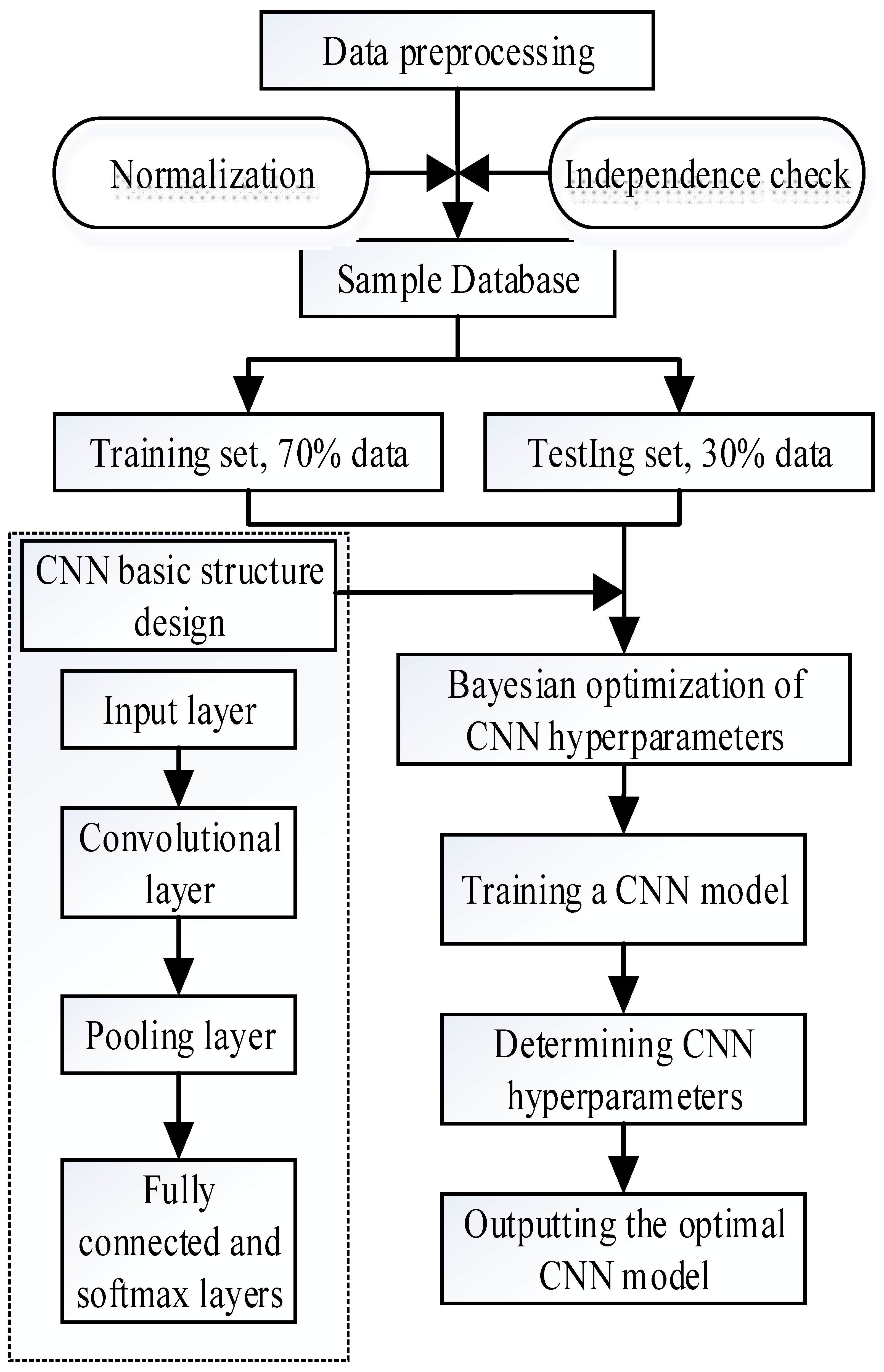
2.1. Convolutional Neural Networks for Bayesian Optimization

Convolutional Neural Networks are an important component of deep learning, originating from the research of Hunel and Wiesel in 1962 and evolving on that basis to become the benchmark for deep learning today [44]. From a theoretical perspective, a convolutional neural network can be a good description of complex nonlinear relationships, and it is a feedforward neural network with better fault tolerance. Convolutional neural networks primarily comprise an input layer, a convolutional layer, a pooling layer, an activation layer, and a fully connected layer [43]. Based on the convolutional layer, a simple linear expression is formed by stacking the operational layers of convolution, pooling, and upsampling, and the fully connected layer is activated by employing the Softmax function to realize the binary classification problem [45,46].
Bayesian optimization (BO) is capable of quickly and accurately finding the optimal solution of the model hyperparameters through multiple iterations and further optimizing the model, such that BO takes on critical significance in parameter combination optimization. It is adopted to deal with the complex mapping relationship between the model fitting parameters and the objective function [41], which satisfies Equation (1):
Z * = arg max z Z f ( z )
where Z* denotes the global optimum of f(z).
Landslide susceptibility is used to predict the possibility of a landslide occurring in a certain place based on multiple environmental factors. Thus, the landslide susceptibility model should be constructed with powerful feature extraction, probability prediction, and a linear regression fitting function. In this study, we adopted the deep learning method for model construction, in which the CNN possesses a better function in model construction, which can be subjected to the highly nonlinear landslide prediction to reduce the overfitting phenomenon of the model. Moreover, there are many types of factors for the occurrence of landslides, and the direct processing of the original factor data will bring considerable inconvenience to the model operation, which will waste more computing power and lead to a reduction in the accuracy of the prediction model. For this reason, in this study, by grading the factors and using the Pearson correlation coefficient for the initial screening of landslide factors, we obtained the dataset after screening, normalized the dataset to obtain the feature vectors, adopted the convolution kernel to extract the feature vectors, and then employed the BO algorithm to search for optimization of the hyperparameters of the CNN. Lastly, we obtained the prediction results by computing the fully connected layer. As shown in Figure 1

2.2. Random Forests

In 2001, Breiman L. and Cutler A. introduced Random Forest for the first time with decision trees, sampling, pruning techniques, stochastic subspaces, and their related statistical principles [47]. This intelligent combinatorial classification algorithm not only possesses good data mining skills but also predicts complex problems more accurately. RF is a model that uses multiple decision trees as classifiers to carry out training and prediction. The model’s accuracy is necessary and linked to the selection of model parameters. The manual tuning of the parameters is time-consuming and unsatisfactory. Accordingly, the BO algorithm is selected to perform hyper-parameter tuning to construct the BO RF model.

2.3. Support Vector Machines

The support vector machine classification method was completely proposed at the end of the 20th century SVM classification [48,49]. Due to the nonlinear transformation of the inner product function, the optimal hyperplane satisfying the classification is searched in the high-dimensional feature space. PSO is a computational method that has been used for optimization processing, with the advantages of fast computing speed and easy implementation [50]. In this way, the PSO algorithm can be applied to the support vector machine to find the optimal SVM parameters through the particle swarm, and each particle moves iteratively to find the potentially optimal particle swarm, using the constant updating of the particles to find the overall optimal position and to determine the direction of its movement and speed. To balance the global search and local search of the PSO algorithm, inertia weights are introduced, and the model optimization result is finally obtained.

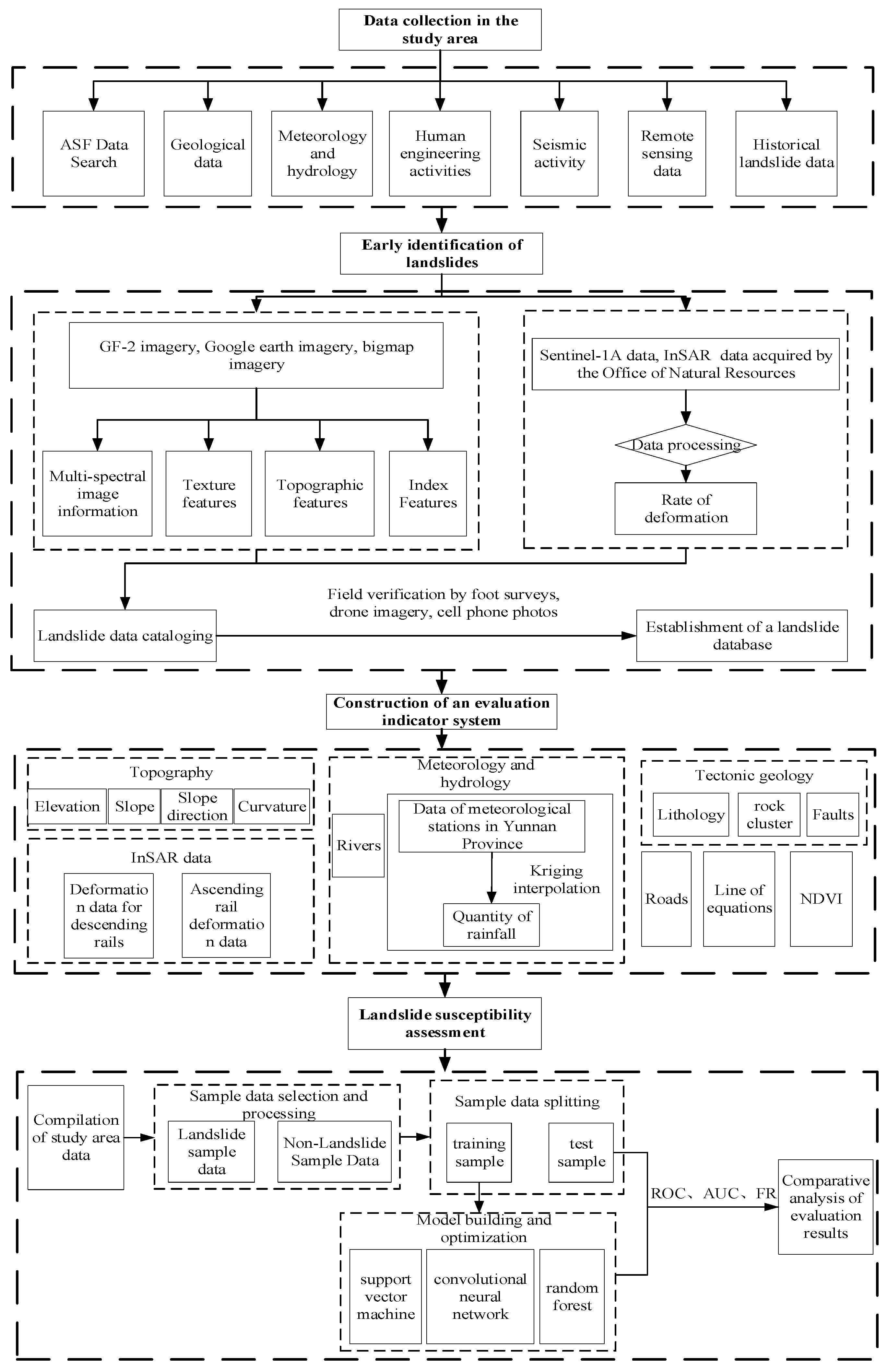
2.4. Technical Routes

In this study, we adopted “3S” technology (“3S” is the collective name for remote sensing (RS), geography information systems (GIS), and global positioning systems (GPS)), InSAR radar technology, and machine learning to study and design the program with the main line of landslide susceptibility evaluation in the study area. Specifically, (1) the data were collected in the study area; (2) landslides were identified in the study area by combining multi-temporal high resolution imagery and InSAR elevation track data; (3) the landslide susceptibility evaluation system was constructed based on the data research and analysis, and the evaluation factors were analyzed and screened by combining the InSAR deformation data, topography and geomorphology, geological formations, hydrological environment, and human engineering activities; (4) the BO-CNN model was constructed, comparison experiments were performed by combining the BO-RF and PSO-SVM models for comparative experiments, we adopted Arcgis software to draw the susceptibility map, the ROC curve AUC value and frequency method were employed to analyze the differences of the models, which can provide theoretical guidance for landslide susceptibility evaluation. The research and technical route of this study are illustrated in Figure 2.

3. Data Preparation and Analysis

3.1. Overview of the Study Area

The study area is located in Gengma, Cangyuan, and Shuangjiang counties in the southwestern part of Lincang City, Yunnan Province, with geographic coordinates between 98°52′ and 99°43′ E longitude and 23°04′ and 24°01′ N latitude (Figure 3). We primarily selected the study area in the region of the 1988 Lancang-Gengma earthquake, and we took the area extending 10 km outside the VII-degree isobar of the Gengma earthquake as the study area. A multitude of landslide geological hazards exist in the study area, and the study placed a major focus on the evaluation and analysis of the landslide geological hazards in the area extending 10 km beyond the VII isoseismic line. The overall terrain of the study area is high on all sides and low in the middle, belonging to the Hengduan Mountain Range with high mountains and valleys. Most of the mountains are north-south; the northeast side of the mountain form is high and steep, with the highest elevation of 2931 m; the southwest is characterized by gullies and ravines, with the lowest elevation of 676 m; the height difference of the entire study area is 2255 m; and most of the terrain slope is 15°~25°. Located in the Indian plate and the Eurasian plate collision zone of the southern extension of the Himalayan rift, frequent earthquakes, the geological and tectonic landscape is more complex, and it is located in the southern section of the Hengduan mountain system, located in the low latitude of the Tropic of Cancer. Moreover, the sun’s altitude angle is large, the range of change is small, and the intersection of the northern tropics and subtropical south of the combination of the Indian Ocean is mainly subjected to the impact of the warm and humid climate and the southwestern monsoon, as well as the formation of the dry and wet seasons. Thus, the vast majority of valleys and slopes are located in the soft rock slope zone, providing favorable topographic conditions for the occurrence of landslides [51].

3.2. Landslide Cataloging

Landslide cataloging data are the prerequisite for landslide susceptibility evaluation, and the completeness and accuracy of the data is of great significance to landslide susceptibility evaluation. In this study, based on the topography, geological structure, and landslide ledger data of the study area, the landslide dataset was established through field validation by synthesizing a variety of new technological methods, such as InSAR deformation rate, high-resolution satellite remote sensing, and unmanned aerial vehicle (UAV) remote sensing. A total of 122 geologic landslides were identified (Figure 4), of which 70 landslides, accounting for 57.38% of the total number of landslides, had significant deformations.

3.3. Data Sources

The DEM used in the experiment is ASTER GDEM V2 data product with a resolution of 30 m. The optical image data used included Gaofen-2 (GF-2) with a resolution of 1 m and Google imagery. Landsat 8 data were used to obtain the Normalized Vegetation Index (NDVI), and the Sentinel-1A data with a resolution of 5 m × 20 m and polarization mode of VV were adopted to obtain the surface deformation information of the study area. Detailed data sources are listed in Table 1.

3.4. Selection of Evaluation Factors

Environmental conditions (e.g., strong neotectonic movements, the development of fracture tectonics, structural fragility of geotechnical bodies, differential climate, and high seismic activity) can lead to geologic hazards (e.g., landslides, avalanches, and mudslides). The main factors in geotechnical proximity conditions cover landslides, vegetation cover, and the influence of human activities. Elevation is presented in Figure 5a. Slope (Figure 5b) is one of the important factors influencing landslides and an important parameter for assessing landslide susceptibility [52], which reflects the degree of inclination of the surface and can be used to measure the efficiency of material flow and energy transfer at the surface. Slope orientation (Figure 5c) takes on greater significance in mountain ecology [53]. Different slope orientations cause differences in temperature, humidity, rainfall, sunshine hours, and solar radiation intensity, which lead to differences in surface cover, which in turn causes differences in the effects of physical weathering and chemical differentiation, affecting the occurrence of landslides. Curvature (Figure 5d) is a factor that measures the change in distortion of the terrain surface, which is used to characterize the change in surface curvature in the vertical direction and to better reflect the complexity of the ground surface [54]. The curvature is calculated as Equation (2).
K v = p 2 r + 2 p q s + q 2 t ( p 2 + q 2 ) ( 1 + p 2 + q 2 ) 3 2
where p is the rate of change in elevation in the x-direction; q is the rate of change in elevation in the y-direction; r is the rate of change in elevation in the x-direction; s is the rate of change in elevation in the x-direction and y-direction; t is the rate of change in elevation in the y-direction.
A large amount of precipitation (Figure 5e) will cause severe damage in the valley; precipitation will destroy the structure and material in the valley, and it may also change the landscape of the valley and cause changes in the vegetation and water, which may ultimately result in collapse, landslides, and mudslides in the valley. Vegetation is an important factor affecting the occurrence of landslides, which prevents soil erosion while improving the stability of slopes, regulating the climate, and reducing the wind speed, thus playing the role of fixing slopes and preventing the loss of soil by scouring. In this study, we used the NDVI (Figure 5f) as the surface vegetation cover status. NDVI satisfies Equation (3).
N D V I = ρ N I R ρ R E D ρ N I R + ρ R E D
where ρNIR is the reflectance in the mid-infrared band; ρRED is the reflectance in the near-infrared band.
The stability of mountain slopes is greatly affected by the large-scale construction of roads (Figure 5g), which leads to more landslides on mountain slopes. Erosion, hollowing out, and wave impacts by rivers (Figure 5h) will cause the rock layers at the bottom of valleys to be pushed away, resulting in cliffs at the bottom of valleys and creating a favorable environment for landslides to develop. Stratigraphic lithology (Figure 5i) is the material basis for the occurrence of landslides. Fractures (Figure 5j) play a significant role in the nurturing of landslides, and they are critical to the stability and security of the earth. Earthquakes (Figure 5k) can cause sudden loss of equilibrium in geotechnical bodies, collapse, and landslides. They can also cause slopes to be in a state of limiting equilibrium or to form landslide hazards and dangerous rock bodies. Thus, geologic hazards can easily be induced or aggravated in the vicinity of zones of strong seismic activity. As fractures continue to expand, they will severely destabilize the rock and soil on the upper and lower walls, and the entire surface, leading to more landslides. In the application of geohazard deformation monitoring, the displacement condition and spatial distribution of the deformation zone can be recognized by the InSAR deformation rate (Figure 5l,m).
Thirteen factors, including elevation, slope, slope direction, curvature, average annual rainfall, vegetation normalization index, stratigraphic lithology, distance from rupture, isokinetic line, distance from river, distance from road, deformation rate of descending rail, and deformation rate of ascending rail are selected as the evaluation factors of landslide susceptibility. The continuity data in the 13 evaluation factors are graded and processed. The discrete data are graded in accordance with the actual determination of the state, and the distribution map is shown in Figure 5.

3.5. Independence Test

Considering the possible correlation between the indicator factors, it is necessary to select the indicator factors through multiple covariance analysis. In this study, by obtaining the landslide data and the evaluation factors in the study area, we tested the evaluation factors for mutual independence using the band set statistical tool in ArcGIS software and obtained their correlation coefficients (ρ = covariance/standard deviation) to ensure the accuracy of the evaluation model of landslide susceptibility. ρ < 0.3 represents the uncorrelation between the factors, 0.3 ≤ ρ < 0.5 represents low correlation, 0.5 ≤ ρ < 0.8 represents medium correlation, and ρ ≥ 0.8 represents high correlation.
As depicted in Table 2, the correlation coefficients were all less than 0.3, which indicates that the evaluation factors are independent of each other, and all 13 evaluation factors can be included in the evaluation model.

3.6. Evaluation Factor Analysis

In this study, we selected 30 m × 30 m resolution raster cells for evaluation, totaling 3,931,814 rasters in the study area. The matrix arrangement of raster cells enabled them to store, retrieve, and recall information easily, such that it has been extensively noticed and emphasized by academics [55]. Frequency Ratio (FR) refers to a variable statistical analysis technique used to measure the probabilistic relationship of multiple influencing factors, which can better identify the key factors for landslides and can more accurately predict the trend of landslide development. The FR method can more accurately identify the correlation between the factors, in which the value of the FR value is dependent on the characteristics of multiple influencing factors. FR is calculated as Equation (4). When the FR value exceeds 1, the correlation between the factors is strong; when the FR value is less than 1, the correlation between the factors is weak [56].
F R ( X i j ) = ( N i j / N ) / ( S i j / S )
where i is the serial number of the evaluation factor; j is the serial number of the secondary classification; Nij denotes the number of landslide rasters occurring in the ith evaluation factor j class; N represents the total number of rasters of landslides in the study area; Sij No. is the number of rasters in the interval of the ith evaluation factor j class; S expresses the total number of rasters in the study area.
As depicted in Table 3, the points of landslide distribution in the mid-mountain region were significantly higher than those in the low-mountain region, and the FR value in the low-mountain region was larger than that in the mid-mountain region, with a value of 1.35. According to the elevation of this class classification, the landslide development significantly contributed to the low-mountain region. The FR value showed a positive correlation with the slope, and the FR value increased with the increase in the slope. FR values exceeded 1 in southeast, south, southwest, and west slopes, with the southeast and southwest slopes contributing the most to landslide occurrence, with FR values of 1.40 and 1.78, respectively. The FR values exceeded 1 in the Kv ≤ 0 region of the study area, with a value of 1.05, which suggested that Kv ≤ 0 can have an effect on landslide occurrence. The average annual rainfall in the regions of <1200 mm, 1200–1300 mm, 1400–1500 mm and >1600 mm had FR values over 1. The landslide FR tended to decline with the increase in NDVI, and the landslide frequency ratios of NDVI in the area of 0–0.6 exceeded 1, with a higher FR in the area of 0–0.3 with a FR value of 2.54. The area was mostly comprised of water bodies, bare land, cultivated land, and construction land, and human activities were relatively concentrated, which can exert a more pronounced effect on the slope and can be prone to landslides.
With the increase in distance from the road and the river, the FR value tended to decrease gradually. In the distance from the road and the river (0–200 m), the FR value was the largest at 3.24 and 2.87, respectively. Due to the influence of human engineering activities on both sides of the river, the stability of the slope was destroyed, making the region prone to landslides. The FR values of P1d, C1pz, and Eγδπ lithologies in the study area all exceeded 1, which indicated that these lithologies can play a certain role in landslide breeding. Specifically, the Eγδπ lithology had the most significant influence, with an FR value of 7.10, and the formation was old tertiary quartz amphibole porphyritic. There was an obvious statistical relationship between the distance from the fracture and landslides; with the distance from the fracture becoming farther, the FR value tended to be smaller. When the distance from the fracture was 300 m, the FR value reached the largest, which was about 1.19, which indicated that the closer the distance from the fracture, the more prone it was to landslides. The study area was mainly distributed in the (−5,5] mm/y area, accounting for 47.10%, and the FR value exceeded 1 in the regions of less than −50 mm/y, (5,10] mm/y, and greater than 10 mm/y, among which the FR value of <−50 mm/y area was the largest, with a value of 12.50. The reason for the above result is that the area of the settlement zone occupies a very small area, whereas the landslides are partially distributed in its area, resulting in a large FR value.

4. Analysis of Evaluation Results

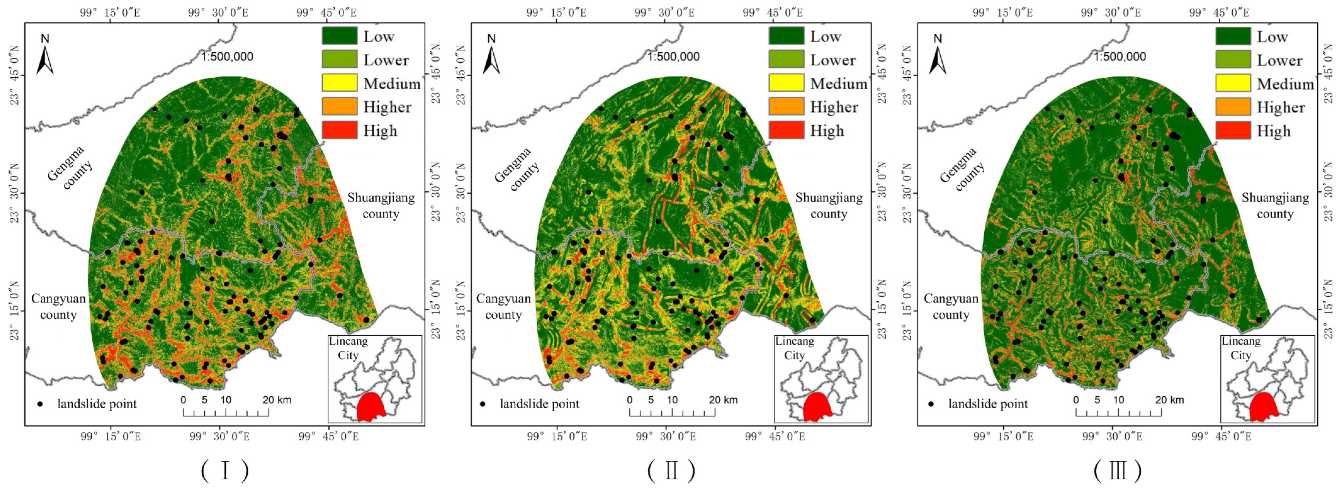
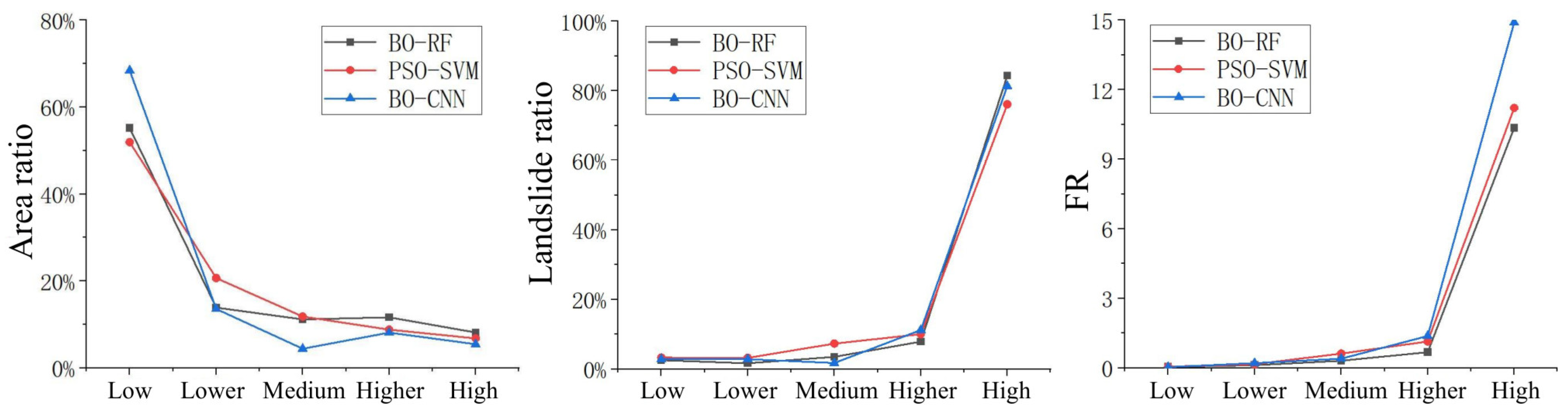
4.1. Results of the Vulnerability Evaluation

After grading the evaluation factors, the graded information values corresponding to the 13 evaluation factors and the superimposed total information values are obtained. Since the evaluation factors have different scales, distribution spaces, and values, the evaluation factors are normalized to unify the data to facilitate better data processing by the model. The commonly used method for normalization is min-max, which is calculated by the formula:
X* = (XXmin)/(XmaxXmin),
where Xmax and Xmin represent the maximum and minimum values of the dataset. In this study, 13 evaluation factors are selected to establish a sample dataset, which includes landslide samples and non-landslide samples. A binary classification model was constructed to assign a value of “0” to the non-landslide unit and a value of “1” to the landslide unit. The sample data were divided into training dataset and test dataset according to 7:3. The training dataset was used for modeling operations, and the test dataset was used for model accuracy testing.
In this study, we used python3.8 software to train the random forest model, import the samples into the software, divide the training dataset, and test the dataset by using the random forest classifier, the training dataset for modeling, to optimize the model before modeling, and search for the optimal hyper-parameter values by using the Bayesian optimization algorithm, which mainly focuses on the hyper-parameters such as n_estimators, max_depths, n_estimators, max_depths, min_samples_splits, and max_features to obtain their optimal parameter values. The values of hyperparameters through 64 iterations are max_depth = 18, min_samples_split = 3, min_samples_leaf = 1, and max_features = 1. The parameters are inputted into the model, and the modeling operation is conducted to obtain the landslide susceptibility results.
The accuracy of SVM, on the other hand, depends entirely on the chosen kernel function, and these variables contain linear function, radial basis function (RBF), sigmoid, and polynomial. Due to the better stability and robustness of the RBF radial basis function, the RBF radial basis function is chosen as the kernel function of the prediction model in this study. Parameter selection is the most critical in the support vector machine model, and the parameter selection is directly related to the prediction performance of the model. In this study, an intelligent optimization search was conducted by PSO, which can find the potentially optimal particle swarm through each particle movement iteration and the overall optimal position by using the continuous updating of the particles and determining the direction of its movement and speed. Furthermore, it can balance the global and local searches of the PSO algorithm, introduce inertia weight, and finally obtain the model optimization results. As shown in Table 4, when initializing the particle swarm optimization calculation, the number of particle swarms in it is adjusted to 50, and the highest evolution frequency in it is adjusted to 200. At the same time, the local search ability factor c1 is adjusted to 1.3, the global search ability factor c2 is adjusted to 1.5, and the inertia weight ω is adjusted to 0.6. Furthermore, the initial coefficient wV is adjusted to 1, and the initial coefficient wP is adjusted to 1. After the iteration, the SVM parameter optimization results are obtained as follows: penalty factor C = 1 and kernel parameter gamma = 0.02. Substituting the parameters into the model operation, the landslide susceptibility results are obtained.
In this study, all the landslide evaluation factors are combined together, and each pixel can be regarded as a one-dimensional feature vector. These vectors together constitute a one-dimensional array of the study area. Using the sample data, a ratio of 7:3 was randomly selected to form the training set and test set for model training and construct a one-dimensional convolutional neural network based on keras. Firstly, the one-dimensional sample data consisting of 13 evaluation factors were input into the model. Then, a size 3 convolutional layer was constructed, and 32, 64, and 128 kernel 3 filters were selected for feature extraction, respectively. An average size 2 pooling layer was then defined behind each convolutional layer while keeping the output dimension unchanged to extract the salient features and at the same time reduce the parameters. In accordance with the work of Sigmoid, ReLU, and Leaky ReLU, who used the tanh activation function for comparison experiments, after comparison, we selected the tanh activation function, using the Bayesian optimization algorithm to adjust the model hyper-parameters to optimize the performance of the model, obtaining batch size = 128 and epoch = 200, which were the best results. The result of landslide susceptibility was then obtained by substituting the parameters.
To determine the processing and visualization of the landslide susceptibility prediction results, ArcGIS10.2 software combined with the resultant data obtained from the model was used. The predicted values of the dataset were then converted into raster image elements through the point-to-raster in the conversion tool of the software. Following this, the landslide susceptibility evaluation value of the whole study area was graded by using the natural segment point method of the software and divided into five susceptibility grade intervals: low susceptibility zone, lower susceptibility zone, medium susceptibility zone, higher susceptibility zone, and high susceptibility zone. The landslide susceptibility maps of the PSO-SVM, BO-RF, and BO-CNN models are shown as (I), (II), and (III) in Figure 6, respectively. By observing the landslide susceptibility maps predicted by the three models, all of them have similar spatial distributions, with high susceptibility zones mainly distributed in the southwestern part of the study area and low susceptibility zones mainly distributed in the northwestern part of the study area.

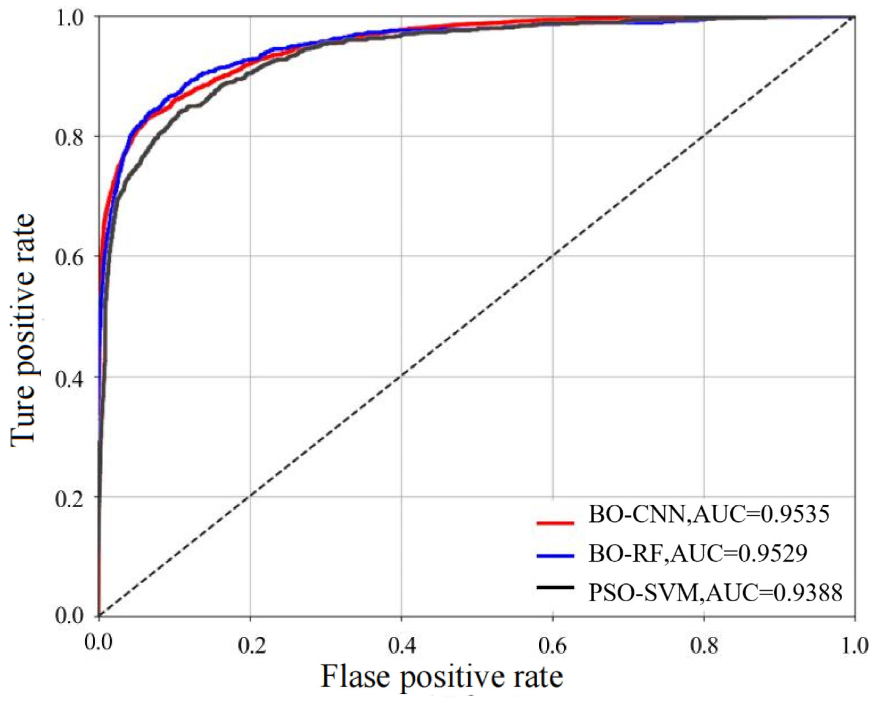
4.2. Evaluation Accuracy Analysis

To comprehensively evaluate the performance of the model in this study area, we conducted an additional validation analysis by using the receiver operating characteristics (ROC) curve and the area under the curve (AUC) value based on the approach by Aleksova et al. [57]. We used the AUC value as an indicator of the probabilistic model’s quality, signifying its reliability in predicting the occurrence or non-occurrence of events. In general, when the AUC value was lower than 0.5, the model had no prediction ability; when the AUC value was 0.5–0.7, the model possessed lower prediction ability; when the AUC value was 0.7–0.9, the model possessed higher prediction ability; when the AUC values exceeded 0.9, the model had very high prediction ability. The ROC curve is plotted with the true positive rate as the horizontal coordinate and the true negative rate as the vertical coordinate, which satisfy Equations (6) and (7).
T P R = T P T P + F R ,
F P R = F P T N + F P ,
where TPR denotes the true positive rate; FPR represents the false positive rate; TP is the number of true positives; FP is the number of false positives; FR expresses the number of false negatives; and TN is the number of true negatives.
The ROC curve and AUC value for this study were computed by using Python statistical software, which is depicted in Figure 7. Our calculations indicated that the ROC curves drawn by the PSO-SVM, BO-RF, and BO-CNN models were all close to the inflection point at the upper left corner, which indicated that all three models can effectively evaluate the landslide susceptibility. The AUC values of PSO-SVM, BO RF, and BO-CNN models also reached 0.9388, 0.9529, and 0.9535, which suggested a commendable level of accuracy for the employed model.
Through reclassification in the Spatial Analyst tool in ArcGIS 10.2 software, the raster image elements and the number of landslides in the geologic landslide susceptibility zones of the study area were counted, and the results of landslide hazard susceptibility in the study area were analyzed using the FR method. As depicted in Figure 8, the prediction results of the PSO-SVM, BO-RF, and BO-CNN models were classified into five categories of susceptibility zones, namely, high, high, medium, low, and low, using the natural breakpoint method. The area of landslide susceptibility in the low susceptibility zones of the BO-CNN model accounted for 68.43% of the total area, and the area of the low susceptibility zones was larger than that of BO-RF and PSO-SVM, while the area of the high susceptibility zones accounted for 5.46% of the total area and the area of high susceptibility zones accounted for 5.46% of the total area. Furthermore, the area of the high susceptibility zone was smaller than that of BO-RF and PSO-SVM; the distribution of landslides in each susceptibility zone was relatively the same in each model, and the proportion of landslides in the high susceptibility zones reached 76.10%, 84.39%, and 81.37%, respectively. The frequency ratios of BO-CNN in the high susceptibility zones and higher susceptibility zones exceeded 1, and those in the middle susceptibility zones, lower susceptibility zones, and lower susceptibility zones were less than 1, with the value of the frequency ratio in the high susceptibility zone being the highest. The frequency ratio of BO-CNN in the high susceptibility zone and the higher susceptibility zone exceeded 1. The frequency ratio of BO-CNN in the middle susceptibility zone, lower susceptibility zone, and low susceptibility zone was less than 1, in which the frequency ratio of the high susceptibility zone was the highest, with a value of 14.90, higher than that of BO-RF and PSO-SVM, whose frequency ratios in the high susceptibility zone were 10.35 and 11.21, respectively. The latter suggested that the BO-CNN model possesses high accuracy in the prediction of landslide susceptibility.

5. Discussion

Geological hazards are a dynamic process from conception through development to stabilization (cessation). With the passage of time, the situation of geological hazards may change, possibly greatly, or produce new geological hazards. Specifically, the old geological hazards have been effectively managed to stabilize, or neglected to manage, protect, and gradually deteriorate. Thus, long-term deformation observation should be performed, monitoring its movement situation, to carry out governance or prevention and effectively reduce the losses caused by this type of disaster.
Since the landslide process is dynamic, we combined the geological background of a pregnant disaster, high-resolution optical remote sensing images, SAR satellite images, and other technical means to identify landslides in the study area for constructing the landslide susceptibility evaluation model. We also adopted on-site surveys and unmanned aerial vehicle (UAV) technology to investigate the situation of landslides and geologic hazards in the study area, which laid the foundation for the evaluation of the susceptibility of landslides. The InSAR deformation rate and other conventional factors served as evaluation factors at the same time, and the Pearson correlation coefficient was adopted to exclude the covariance factor to construct the CNN landslide susceptibility evaluation model with powerful feature extraction, probability prediction, and linear regression fitting functions. Next, we used the BO algorithm to seek the optimization of the hyper-parameters of the CNN to establish the BO-CNN landslide susceptibility model, which increased the stability of the model and thus improved the model accuracy.
Despite the improvement in the model’s accuracy and robustness, this study also has limitations. Firstly, we only adopted the raster unit for evaluation instead of other units for evaluation and comparative analysis, and the research based on other evaluation units should be further strengthened. Secondly, when we built the landslide susceptibility model, due to the many internal and external factors for the evolution of landslides, the selected evaluation index factors had certain limitations; therefore, in subsequent research, the experiment should be optimized in the selection of evaluation factors to build a more comprehensive and accurate prediction model.

6. Conclusions

In this study, the aim was to address the problems of limited data sources for traditional landslide monitoring methods and the lack of effective methods to excavate the spatial distribution characteristics of landslide disasters and their triggering factors. We presented a landslide susceptibility evaluation method by considering InSAR deformation. The presented method uses historical landslide data, high-resolution satellite remote sensing, unmanned aircraft remote sensing, and surface deformation information of the study area by inverting the InSAR technology, combining engineering geology principles and landslide interpretation signs for the early identification of regional landslides. Moreover, we established 122 landslide databases after field verification. After screening, we selected 13 evaluation factors (i.e., elevation, slope, slope direction, curvature, average annual rainfall, vegetation normalization index, stratigraphic lithology, distance from faults, line of equations, distance from rivers, distance from roads, and rate of descending and ascending deformation), and we developed an evaluation index system by using the above-mentioned factors to build a dataset of landslides in the study area. Next, we evaluated the susceptibility of landslides in the study area by using the BO-CNN model from the perspective of disaster prevention and mitigation.
We tested the screened evaluation factors for independence. The 13 evaluation factors were independent of each other, which can ensure the accuracy of the susceptibility model. We analyzed the relationship between landslides and indicator factors based on the frequency ratio method by grading all evaluation factors. The results indicated that the categories of the impact factors identified by using the frequency-ratio model included the elevation of low mountains, slope gradient of sharp, steep and dangerous slopes, slope direction of south-east and south-west slopes, topographic curvature less than or equal to 0, average annual rainfall of less than 1300 mm, 1400–1500 mm and more than 1600 mm, NDVI 0–0.6, distance from roads 0–400 m, distance from rivers 0–400 m and 600–800 m, the stratigraphic lithology of P, C, Eγδπ, the distance from the fault of 0–300 m and more than 1200 m, the isoseismic line of Ⅶ and Ⅶ outside (10 km), the rate of deformation of the descending rail of more than −5 mm/y, and the rate of deformation of the ascending rail of less than −50 mm/y and more than 5 mm/y, which can indirectly or directly contribute to the occurrence of landslides.
We implemented PSO-SVM, BO-RF, and BO-CNN landslide susceptibility models by using the Python programming language, and we carried out susceptibility evaluation. To determine the accuracy of the models, we selected ROC and AUC as the model accuracy indicators in this study. The calculation results indicated that the ROC curves of the three models were close to the upper left corner, and the AUC values of the three models reached 0.9388, 0.9529, and 0.9535, respectively. Specifically, the BO-CNN model obtained the most effective ROC curve and AUC value. We analyzed the distribution of susceptible zones in the study area, and we adopted the three models and the FR to validate the feasibility of the models with the percentage of the number of landslides in the susceptible zones predicted. The experimental results revealed that the proportion of landslides in the high susceptibility zone of PSO-SVM, BO-RF, and BO-CNN reached 76.10%, 84.39%, and 81.37%, respectively, which indicated that the landslides in the study area were primarily distributed in the high susceptibility zone in line with the actual situation. Furthermore, the FR value of landslides in the high susceptibility zone of BO-CNN reached up to 14.9, and the FR value was pronouncedly higher than 1, which can validate a stronger correlation. The combination of the two situations suggested that the BO-CNN model can be used for landslide susceptibility evaluation with high accuracy.

Author Contributions

Conceptualization, Y.D. and Y.L.; methodology, Y.D.; software, Y.D.; validation, X.Z. (Xincheng Zhou) and Y.D.; formal analysis, Y.D.; investigation, Y.D. and X.Z. (Xincheng Zhou); resources, X.Z. (Xiaoqing Zuo); data curation, Y.D. and X.Z. (Xincheng Zhou); writing—original draft preparation, Y.D.; writing—review and editing, Y.D., X.Z. (Xiaoqing Zuo) and Y.L.; visualization, Y.D.; supervision, X.Z. (Xiaoqing Zuo); project administration, X.Z. (Xiaoqing Zuo); funding acquisition, X.Z. (Xiaoqing Zuo). All authors have read and agreed to the published version of the manuscript.

Funding

This research was funded by The National Natural Science Foundation of China, grant number 42161067.

Data Availability Statement

Not applicable.

Acknowledgments

The authors sincerely thank the anonymous reviewers for their valuable and constructive comments.

Conflicts of Interest

The authors declare no conflict of interest.

References

  1. Lukić, T.; Leščešen, I.; Sakulski, D.; Basarin, B.; Jordaan, A. Rainfall erosivity as an indicator of sliding occurrence along the southern slopes of the Bačka loess plateau: A case study of the Kula settlement, Vojvodina (North Serbia). Carpathian J. Earth Environ. Sci. 2016, 11, 303–318. [Google Scholar]
  2. Lukić, T.; Bjelajac, D.; Fitzsimmons, K.E.; Marković, S.B.; Basarin, B.; Mlađan, D.; Micić, T.; Schaetzl, R.J.; Gavrilov, M.B.; Milanović, M.; et al. Factors triggering landslide occurrence on the Zemun loess plateau, Belgrade area, Serbia. Environ. Earth Sci. 2018, 77, 519. [Google Scholar] [CrossRef]
  3. Zhuang, J.; Peng, J. A coupled slope cutting—A prolonged rainfall-induced loess landslide: A 17 October 2011 case study. Bull. Eng. Geol. Environ. 2014, 73, 997–1011. [Google Scholar] [CrossRef]
  4. Zhuang, J.; Peng, J.; Wang, G.; Javed, I.; Wang, Y.; Li, W. Distribution and characteristics of landslide in Loess Plateau: A case study in Shaanxi province. Eng. Geol. 2018, 236, 89–96. [Google Scholar] [CrossRef]
  5. Morar, C.; Lukić, T.; Basarin, B.; Valjarević, A.; Vujičić, M.; Niemets, L.; Telebienieva, I.; Boros, L.; Nagy, G. Shaping Sustainable Urban Environments by Addressing the Hydro-Meteorological Factors in Landslide Occurrence: Ciuperca Hill (Oradea, Romania). Int. J. Environ. Res. Public Health 2021, 18, 5022. [Google Scholar] [CrossRef]
  6. Chi, T.; Su, Y. Integrated System for Remote Sensing Monitoring and Assessment of Major Natural Disasters; China Science and Technology Press: Beijing, China, 1995. [Google Scholar]
  7. Moretto, S.; Bozzano, F.; Esposito, C.; Mazzanti, P.; Rocca, A. Assessment of landslide pre-failure monitoring and forecasting using satellite SAR interferometry. Geosciences 2017, 7, 36. [Google Scholar] [CrossRef]
  8. Tzouvaras, M.; Danezis, C.; Hadjimitsis, D.G. Small scale landslide detection using Sentinel-1 interferometric SAR coherence. Remote Sens. 2020, 12, 1560. [Google Scholar] [CrossRef]
  9. Tzouvaras, M. Statistical Time-Series Analysis of Interferometric Coherence from Sentinel-1 Sensors for Landslide Detection and Early Warning. Sensors 2021, 21, 6799. [Google Scholar] [CrossRef]
  10. Wasowski, J.; Bovenga, F.; Casarano, D.; Nutricato, R.; Refice, A. Application of PSI techniques to landslide investigations in the Caramanico area (Italy): Lessons learnt. In Proceedings of the Fringe 2005 Workshop; Application of PSI Techniques to Landslide Investigations in the Caramanico Area (Italy), Frascati, Italy, 28 November–2 December 2005; Volume 610. [Google Scholar]
  11. Guzzetti, F.; Reichenbach, P.; Ardizzone, F.; Cardinali, M.; Galli, M. Estimating the quality of landslide susceptibility models. Geomorphology 2006, 81, 166–184. [Google Scholar] [CrossRef]
  12. Cheng, T.; San, X.; Dong, W. A study of landslide distribution in loess area with InSAR. Hydrogeol. Eng. Geol. 2008, 25, 98–101. [Google Scholar]
  13. Carlà, T.; Tofani, V.; Lombardi, L.; Raspini, F.; Bianchini, S.; Bertolo, D.; Thuegaz, P.; Casagli, N. Combination of GNSS, satellite InSAR, and GBInSAR remote sensing monitoring to improve the understanding of a large landslide in high alpine environment. Geomorphology 2019, 335, 62–75. [Google Scholar] [CrossRef]
  14. Ge, D.; Dai, K.; Guo, Z.; Li, Z. Early Identification of serious geological hazards with integrated remote sensing technologies:thoughts and recommendations. J. Wuhan Univ. 2019, 44, 949–956. [Google Scholar]
  15. Manconi, A.; Kourkouli, P.; Caduff, R.; Strozzi, T.; Loew, S. Monitoring Surface Deformation over a Failing Rock Slope with the ESA Sentinels: Insights from Moosfluh Instability, Swiss Alps. Remote Sens. 2018, 10, 672. [Google Scholar] [CrossRef]
  16. Tzouvaras, M.; Danezis, C.; Hadjimitsis, D.G. Differential SAR Interferometry Using Sentinel-1 Imagery-Limitations in Monitoring Fast Moving Landslides: The Case Study of Cyprus. Geosciences 2020, 10, 236. [Google Scholar] [CrossRef]
  17. Xu, Q.; Dong, X.; Li, W. Integrated space-air-ground early detection, Monitoring and warming system for potentianl catastrophic geohazards. J. Wuhan Univ. 2019, 44, 957–966. [Google Scholar]
  18. Shi, X.; Xu, J.; Jiang, H.; Zhang, L.; Liao, M. Slope stability state monitoringandn updating of the outang landslide, Three gorges area with time series InSAR analysis. Earth Sci. 2019, 44, 4284–4292. [Google Scholar]
  19. Liu, B.; Ge, D.; Wang, S.; Li, M.; Zhang, L.; Wang, Y.; Wu, Q. Combining application of TOPS and scanSAR InSAR in large-scale geohazards identification. J. Wuhan Univ. 2020, 45, 1756–1762. [Google Scholar]
  20. Cai, J.H.; Zhang, L.; Dong, J.; Dong, X.; Liao, M.; Xu, Q. Detection and monitoring of post-earthquake landslides in jiuzhaigou using radar remote sensing. J. Wuhan Univ. 2020, 45, 1707–1716. [Google Scholar]
  21. Dai, C.; Li, W.L.; Lu, H.Y.; Yang, F.; Xu, Q.; Jian, J. Active landslides detection in Zhouqu county, gansu province using InSAR technology. J. Wuhan Univ. 2021, 46, 994–1002. [Google Scholar]
  22. Zhang, C.L.; Li, Z.H.; Yu, C.; Song, C.; Xiao, R.; Peng, J. Landslide detection of the jinsha river region using GACOS assisted InSAR stacking. J. Wuhan Univ. 2021, 46, 1649–1657. [Google Scholar]
  23. Li, M.; Zhang, L.; Dong, J.; Cai, J.; Liao, M. Detection and monitoring of potential landslides along Minjiang river valley in maoxian county, sichuan using radar remote sensing. J. Wuhan Univ. 2021, 46, 1529–1537. [Google Scholar]
  24. Zhou, D.; Zuo, X.; Xi, W.; Xiao, B.; Bi, R.; Xin, F. Early identification of landslide hazards in deep-cut alpine canyon using SBAS-InSAR technology. Chin. J. Geol. Hazards Prev. 2022, 33, 16–24. [Google Scholar]
  25. He, J.; Ju, N.; Xie, M.; Wen, Y.; Zuo, M.; Deng, M. Comparison of InSAR technology for identification of hidden dangers of geological hazards in alpine and canyon areas. Earth Sci. 2023, 1–20. [Google Scholar]
  26. Jiang, Z.; Zhao, C.; Yan, M.; Wang, B.; Liu, X. The Early Identification and Spatio-Temporal Characteristics of Loess Landslides with SENTINEL-1A Datasets: A Case of Dingbian County, China. Remote Sens. 2022, 14, 6009. [Google Scholar] [CrossRef]
  27. Zhou, P.; Deng, H.; Zhang, W.J. Landslide susceptibility evaluation based on information value model and machine learning method: A case study of lixian county, sichuan province. Geoscience 2022, 42, 1665–1675. [Google Scholar]
  28. Luo, L.; Pei, X.; Cui, S.; Huang, R.; Zhu, L.; He, Z. Combined selection of susceptibility assessment factors for Jiuzhaigou earthquake-induced landslides. J. Rock Mech. Eng. 2021, 40, 2306–2319. [Google Scholar]
  29. Zhang, Z.; Dang, M.; Xu, S.; Zhang, Y.; Fu, H.; Li, Z. Comparison of landslide susceptibility assessment models in Zhenkang County, Yunnan Province, China. J. Rock Mech. Eng. 2022, 41, 157–171. [Google Scholar]
  30. Li, Y.; Xu, L.; Zhang, L. Study on development patterns and susceptibility evaluation of coseismic landslides within mountainous regions Influenced by strong earthquakes. Earth Sci. 2023, 48, 1960–1976. [Google Scholar]
  31. Boussouf, S.; Fernández, T.; Hart, A.B. Landslide susceptibility mapping using maximum entropy (MaxEnt) and geographically weighted logistic regression (GWLR) models in the Río Aguas catchment (Almería, SE Spain). Nat. Hazards 2023, 117, 207–235. [Google Scholar] [CrossRef]
  32. Huang, W.; Ding, M.; Li, Z.; Zhuang, J.; Yang, J.; Li, X.; Meng, L.; Zhang, H.; Dong, Y. An Efficient User-Friendly Integration Tool for Landslide Susceptibility Mapping Based on Support Vector Machines: SVM-LSM Toolbox. Remote Sens. 2022, 14, 3408. [Google Scholar] [CrossRef]
  33. Huang, W.; Ding, M.; Wang, D.; Jiang, L.; Li, Z. Landslide susceptibility assessment along the Sichuan-Tibet transportation corridor based on layer adaptive weighted convolutional neural network. Earth Sci. 2022, 47, 2015–2030. [Google Scholar]
  34. Huan, Y.; Song, L.; Khan, U.; Zhang, B. Stacking ensemble of machine learning methods for landslide susceptibility mapping in Zhangjiajie City, Hunan Province, China. Environ. Earth Sci. 2022, 82, 35. [Google Scholar] [CrossRef]
  35. Kong, J.; Zhong, J.; Peng, J.; Zhan, J.; Ma, P.; Mu, J.; Wang, J.; Wang, S.; Zheng, J.; Fu, Y. Evaluation of landslide susceptibility in chinese loess plateau based on IV-RF and IV-CNN coupling models. Earth Sci. 2023, 48, 1711–1729. [Google Scholar]
  36. Hidayatul, M.U.; Rohmaneo, M.D. Landslide Susceptibility Spatial Modelling Using Random Forest Algorithm: A Case Study of Malang Regency. IOP Conf. Ser. Earth Environ. Sci. 2023, 1127, 012026. [Google Scholar]
  37. Gui, J.; Alejano, L.; Yao, M.; Zhao, F.; Chen, W. GIS-Based Landslide Susceptibility Modeling: A Comparison between Best-First Decision Tree and Its Two Ensembles ( BagBFT and RFBFT). Remote Sens. 2023, 15, 1007. [Google Scholar] [CrossRef]
  38. Teruyuki, K.; Koki, S.; Satoshi, N.; Takahashi, K. Landslide susceptibility mapping using automatically constructed CNN architectures with pre-slide topographic DEM of deep-seated catastrophic landslides caused by Typhoon Talas. Nat. Hazards 2023, 117, 339–364. [Google Scholar]
  39. Behnia, P.; Blais-Stevens, A. Landslide susceptibility modelling using the quantitative random forest method along the northern portion of the Yukon Alaska Highway Corridor, Canada. Nat. Hazards 2018, 90, 1407–1426. [Google Scholar] [CrossRef]
  40. Phong, T.; Phan, T.; Prakash, I.; Singh, S.K.; Shirzadid, A.; Chapi, K.; Ly, H.-B.; Ho, L.S.; Quoc, N.K.; Pham, B.T. Landslide susceptibility modeling using different artificial intelligence methods: A case study at Muong Lay district, Vietnam. Geocarto Int. 2021, 36, 1685–1708. [Google Scholar] [CrossRef]
  41. Wang, S.; Zhuang, J.; Zheng, J.; Fan, H.; Kong, J.; Zhan, J. Application of Bayesian Hyperparameter Optimized Random Forest and XGBoost Model for Landslide Susceptibility Mapping. Front. Earth Sci. 2021, 9, 712240. [Google Scholar] [CrossRef]
  42. Zhang, Y.; Xu, P.; Liu, J.; He, J.; Yang, H.; Zeng, Y.; He, Y.; Yang, C. Comparison of LR, 5-CV SVM, GA SVM, and PSO SVM for landslide susceptibility assessment in Tibetan Plateau area, China. J. Mt. Sci. 2023, 20, 979–995. [Google Scholar] [CrossRef]
  43. Wu, X.; Yang, J.; Niu, R. A Landslide susceptibility assessment method using SMOTE and convolutional neural network. J. Wuhan Univ. 2020, 45, 1223–1232. [Google Scholar]
  44. Hubel, D.H.; Wiesel, T.N. Receptive fields, binocular interaction and functional architecture in the cat’s visual cortex. J. Physiol. 1962, 160, 106. [Google Scholar] [CrossRef] [PubMed]
  45. Lorenzo, N.; Kushanav, B.; Raj, S.M.; Monserrat, O.; Catani, F. Rapid Mapping of Landslides on SAR Data by Attention U-Net. Remote Sens. 2022, 14, 1449. [Google Scholar]
  46. Ghorbanzadeh, O.; Meena, R.S.; Blaschke, T.; Aryal, J. UAV-Based Slope Failure Detection Using Deep-Learning Convolutional Neural Networks. Remote Sens. 2019, 11, 2046. [Google Scholar] [CrossRef]
  47. Breiman, L. Random forests. Mach. Learn. 2001, 45, 5–32. [Google Scholar] [CrossRef]
  48. Vapnik, V.; Lerner, A. Pattern recognition using generalized portrait method. Autom. Remote Control 1963, 24, 774–780. [Google Scholar]
  49. Vapnik, V. The Nature of Statistical Learning Theory; Springer: Berlin/Heidelberg, Germany, 2000. [Google Scholar]
  50. Sunil, S.; Anik, S.; Bishnu, R.; Raju, B.; Dhruv, B.; Barnali, K. Correction to: Integrating the Particle Swarm Optimization (PSO) with machine learning methods for improving the accuracy of the landslide susceptibility model. Earth Sci. Inform. 2022, 15, 2663–2664. [Google Scholar]
  51. Zou, S.; Duan, H. Study on the distribution pattern of geologic hazards in Gengma County, Yunnan Province. Sichuan J. Geol. 2016, 36 (Suppl. S1), 38–41, 46. [Google Scholar]
  52. Gorokhovich, Y.; Machado, E.A.; Melgar, L.I.G.; Ghahremani, M. Improving landslide hazard and risk mapping in Guatemala using terrain aspect. Nat Hazards 2016, 81, 869–886. [Google Scholar] [CrossRef]
  53. Qi, W.; Yang, X.; Li, Z.; Li, Y.; Yang, F. Study on the correlation between topographic features and distribution of land use types in Jinggang Mountain. Remote Sens. Inf. 2018, 33, 64–71. [Google Scholar]
  54. Yang, Y.; Li, Z.; Liu, M. Analysis of topographic differences of yongshou county based on different resolutions of DEM. Res. Soil Water Conserv. 2018, 25, 131–136. [Google Scholar]
  55. Xiao, B.; Zhao, J.; Li, D.; Zhao, Z.; Zhou, D.; Xi, W.; Li, Y. Combined SBAS-InSAR and PSO-RF Algorithm for Evaluating the Susceptibility Prediction of Landslide in Complex Mountainous Area: A Case Study of Ludian County, China. Sensors 2022, 22, 8041. [Google Scholar] [CrossRef] [PubMed]
  56. Guo, Z.; Yin, K.; Huang, F.; Guo, Z.; Guo, F.; Lai, P. Evaluation of landslide susceptibility based on landslide classification and weighted frequency ratio model. J. Rock Mech. Eng. 2019, 38, 287–300. [Google Scholar]
  57. Aleksova, B.; Lukić, T.; Milevski, I.; Spalević, V.; Marković, S.B. Modelling Water Erosion and Mass Movements (Wet) by Using GIS-Based Multi-Hazard Susceptibility Assessment Approaches: A Case Study—Kratovska Reka Catchment (North Macedonia). Atmosphere 2023, 14, 1139. [Google Scholar] [CrossRef]
Figure 1. An overview of convolutional neural network with Bayesian optimization used in this research.
Applsci 13 11388 g001
Figure 2. Research technologies routes and research workflow.
Applsci 13 11388 g002
Figure 3. Geographic location of the study area.
Applsci 13 11388 g003
Figure 4. Drone aerial view of landslides.
Applsci 13 11388 g004
Figure 5. Distribution of evaluation factors.
Applsci 13 11388 g005
Figure 6. Landslide susceptibility map. (I): PSO-SVM (II): BO-RF (III): BO-CNN.
Applsci 13 11388 g006
Figure 7. ROC curve and AUC value.
Applsci 13 11388 g007
Figure 8. Distribution of landslides by determined susceptibility classes.
Applsci 13 11388 g008
Table 1. Data sources.
Data CategoriesData ScaleData Time PhaseData Sources
DEM30 m2021ASTER GDEM V2
Slope, slope direction, curvature30 m2021Elevation data acquisition
GF-2 remote sensing imagery1.0 m2020, 2021Yunnan Remote Sensing Center
Google remote sensing imagery--2018–2021Google Earth
Quantity of rainfall30 m2016–2020Yunnan Provincial Bureau of Statistics
Rivers and roads--2020Data from the Third National Land Survey
Stratigraphic lithology and faults1:50,0002015Natural Resources Bureau (NRB)
NDVI30 m2020Landsat 8 data
Sentinel-1A data5 m × 20 m2018.7–2021.5European Space Agency (ESA)
Table 2. Matrix of correlation coefficients of evaluation factors.
EFabcdefghijklm
a1.00
b0.041.00
c0.000.021.00
d0.020.040.021.00
e0.03−0.02−0.040.001.00
f0.130.15−0.200.05−0.031.00
g0.150.090.020.01−0.170.141.00
h0.20−0.010.040.01−0.110.060.121.00
i−0.10−0.14−0.04−0.010.09−0.16−0.12−0.011.00
j−0.04−0.060.010.000.13−0.040.00−0.050.131.00
k0.100.11−0.020.01−0.200.150.12−0.01−0.090.011.00
l−0.110.040.04−0.010.01−0.09−0.02−0.120.020.01−0.031.00
m0.010.03−0.040.010.010.02−0.020.01−0.010.000.010.031.00
Notes: EF: evaluation factors; a: Elevation; b: Slope; c: Slope direction; d: Curvature; e: Quantity of rainfall; f: NDVI; g: Distance from road; h: Distance from river; i: Stratigraphic lithology; j: Distance from faults; k: Line of equations; l: Rate of deformation of the descending rail; m: Rate of deformation of the ascending rail.
Table 3. Evaluation factor grading FR values.
Evaluation FactorsClassificationTypeNijSijSij/SNij/NFR
Elevationlow mountainscontinuous147,862523.76%5.07%1.35
middle mountains3,783,95297396.24%94.93%0.99
Slopeflatcontinuous179,82514.57%0.10%0.02
moderate903,2789522.97%9.27%0.40
incline1,543,19234039.25%33.17%0.85
steep1,018,12833425.89%32.59%1.26
rapid245,0351846.23%17.95%2.88
dangerous42,356711.08%6.93%6.43
Slope directionElsecontinuous10,21500.26%0.00%0.00
north487,4981512.40%1.46%0.12
northeastern485,06911412.34%11.12%0.90
east500,80111712.74%11.41%0.90
southeast509,36718612.96%18.15%1.40
south482,21712312.26%12.00%0.98
southwestern517,23724013.16%23.41%1.78
western479,56112112.20%11.80%0.97
northwest459,8493911.70%3.80%0.33
Curvature≤0continuous2,365,22364760.16%63.12%1.05
>01,566,59137839.84%36.88%0.93
Quantity of rainfall<1200 mmcontinuous396,16522310.08%21.76%2.16
1200~1300 mm853,04324221.70%23.61%1.09
1300~1400 mm962,23911424.47%11.12%0.45
1400~1500 mm806,60523020.51%22.44%1.09
1500~1600 mm692,58311517.61%11.22%0.64
>1600 mm221,179615.63%5.95%1.06
NDVI0~0.30continuous170,3701134.33%11.02%2.54
0.30~0.601,357,29253534.52%52.20%1.51
0.60~0.801,219,98823831.03%23.22%0.75
0.80~0.90471,9446812.00%6.63%0.55
0.90~1.00712,2207118.11%6.93%0.38
Distance from road0~200 mdiscrete407,33234410.36%33.56%3.24
200~400 m333,9671128.49%10.93%1.29
400~600 m298,890777.60%7.51%0.99
600~800 m271,858506.91%4.88%0.71
800~1000 m249,179376.34%3.61%0.57
>1000 m2,370,58840560.29%39.51%0.66
Distance from river0~200 mdiscrete392,2322939.98%28.59%2.87
200~400 m367,3961269.34%12.29%1.32
400~600 m352,797458.97%4.39%0.49
600~800 m333,9751258.49%12.20%1.44
800~1000 m313,162567.96%5.46%0.69
>1000 m2,172,25238055.25%37.07%0.67
Stratigraphic lithologyPt1-2Ldiscrete456,6933611.62%3.51%0.30
T3sc364,912789.28%7.61%0.82
P1d969,09427024.65%26.34%1.07
J2h453,5056211.53%6.05%0.52
D1w254,016606.46%5.85%0.91
C1pz831,43636821.15%35.90%1.70
φω420300.11%0.00%0.00
Qh58,52201.49%0.00%0.00
N1n249,953156.36%1.46%0.23
Eγδπ62,6481161.59%11.32%7.10
O1lj35,96800.91%0.00%0.00
Pz1ln190,864204.85%1.95%0.40
Distance from faults0~300 mdiscrete517,92516113.17%15.71%1.19
300~600 m472,81011012.03%10.73%0.89
600~900 m416,2876610.59%6.44%0.61
900~1200 m362,051819.21%7.90%0.86
>1200 m2,162,74160755.01%59.22%1.08
Line of equationscontinuous284,748647.24%6.24%0.86
560,9749614.27%9.37%0.66
1,456,77040737.05%39.71%1.07
Ⅶ outside (10 km)1,629,32245841.44%44.68%1.08
Rate of deformation of the descending rail<−50 mm/ycontinuous53,11721.35%0.20%0.14
(−50,−30] mm/y98,02622.49%0.20%0.08
(−30,−10] mm/y632,1926816.08%6.63%0.41
(−10,−5] mm/y558,98910614.22%10.34%0.73
(−5,5] mm/y1,376,99141935.02%40.88%1.17
(5,10] mm/y489,34920012.45%19.51%1.57
>10 mm/y723,15022818.39%22.24%1.21
Rate of deformation of the ascending rail<−50 mm/ycontinuous153450.04%0.49%12.50
(−50,−30] mm/y28,60940.73%0.39%0.54
(−30,−10] mm/y489,54810612.45%10.34%0.83
(−10,−5] mm/y528,80611013.45%10.73%0.80
(−5,5] mm/y1,851,89147547.10%46.34%0.98
(5,10] mm/y563,18820414.32%19.90%1.39
>10 mm/y468,23812611.91%12.29%1.03
Table 4. PSO-SVM parameters.
ParametersNoteParametersNote
kernelRBFc11.3
C1c21.5
gamma0.02ω0.6
number of PSO50wV1
frequency200wP1
Disclaimer/Publisher’s Note: The statements, opinions and data contained in all publications are solely those of the individual author(s) and contributor(s) and not of MDPI and/or the editor(s). MDPI and/or the editor(s) disclaim responsibility for any injury to people or property resulting from any ideas, methods, instructions or products referred to in the content.

