YOLOv7-3D: A Monocular 3D Traffic Object Detection Method from a Roadside Perspective

Abstract

Current autonomous driving systems predominantly focus on 3D object perception from the vehicle’s perspective. However, the single-camera 3D object detection algorithm in the roadside monitoring scenario provides stereo perception of traffic objects, offering more accurate collection and analysis of traffic information to ensure reliable support for urban traffic safety. In this paper, we propose the YOLOv7-3D algorithm specifically designed for single-camera 3D object detection from a roadside viewpoint. Our approach utilizes various information, including 2D bounding boxes, projected corner keypoints, and offset vectors relative to the center of the 2D bounding boxes, to enhance the accuracy of 3D object bounding box detection. Additionally, we introduce a 5-layer feature pyramid network (FPN) structure and a multi-scale spatial attention mechanism to improve feature saliency for objects of different scales, thereby enhancing the detection accuracy of the network. Experimental results demonstrate that our YOLOv7-3D network achieved significantly higher detection accuracy on the Rope3D dataset while reducing computational complexity by 60%.

1. Introduction

With the continuous development and intelligence of urban transportation, the safety and efficiency of autonomous driving have become a focal point for researchers [1,2,3,4]. Visual traffic monitoring systems, as an essential component of traffic management and safety, have broad application prospects. These systems [5,6,7,8] utilize cameras and other sensor devices to capture real-time traffic scenes and analyze and process images or videos using computer vision algorithms to extract traffic information and key data. Visual traffic monitoring systems consist of functions such as vehicle detection, vehicle tracking, license plate recognition, and behavior analysis, which are used to extract traffic information and features. Furthermore, they enable functions such as vehicle count, traffic flow monitoring, congestion detection, and traffic accident warning through the utilization of traffic information and features [9,10]. Visual traffic monitoring systems have extensive applications in traffic management, urban planning, and traffic safety. They can assist traffic management departments in better monitoring and managing traffic flow, improving road utilization efficiency, reducing traffic congestion and the probability of accidents, and providing a safer and more convenient traffic environment for urban residents.

Traditional traffic monitoring systems primarily rely on 2D image processing [11,12,13], which can only provide limited information, thereby limiting the accurate recognition and stereo perception capabilities of traffic targets. To address this issue, in recent years, researchers have started to incorporate 3D object detection techniques from the computer vision field into roadside monitoring viewpoints to provide more comprehensive and accurate traffic object information [14,15]. Single-camera 3D traffic object detection, as one of the methods, estimates the three-dimensional positions and orientations of traffic objects based on the texture and contextual information in the images, in the case of a single camera.

There are several advantages to using single-camera 3D object detection in roadside traffic monitoring systems:

(1)

Spatial perception: By using 3D detection, the system can accurately perceive the precise position, size, and orientation information of vehicles, enabling accurate perception of vehicles in three-dimensional space. This helps to better understand vehicle motion behavior and spatial layout.

(2)

Distance estimation: 3D detection provides distance estimation between vehicles and monitoring cameras. This is crucial for evaluating key parameters such as distance, speed, and acceleration between vehicles and cameras. Such information is vital for traffic flow statistics, behavior analysis, and accident warning applications.

(3)

Enhanced safety: Through 3D detection, the monitoring system can more accurately identify the position and motion status of vehicles, providing more reliable traffic information. This helps in the timely detection of traffic violations, abnormal driving behaviors, and accident risks, enabling appropriate warnings and measures to be taken and improving road safety.

(4)

Cost-effectiveness: Compared to multi-sensor fusion solutions, monocular vision systems have lower costs. They only require a single camera to capture image information without the need for additional sensor devices, thereby reducing installation and maintenance costs.

However, the use of a monocular 3D object detection method requires precise camera intrinsic and extrinsic parameters during the model training and deployment process, and the dataset annotation process is more cumbersome. However, these limitations cannot overshadow the advantages of this algorithm.

Moreover, single-camera 3D object detection faces several challenges and difficulties. Firstly, cameras in roadside monitoring systems have different installation heights, pitch angles, and complex road environments. Due to the limitations of a single-camera viewpoint, the camera can only provide a limited field of view, leading to situations where targets are occluded, or there are variations in the viewpoint, thereby increasing the complexity of object detection. Secondly, due to the lack of accurate depth information in images, relying solely on 2D images for object detection makes it difficult to obtain the true size and shape of objects, affecting precise localization and pose estimation. Additionally, environmental factors such as lighting changes and weather conditions can also affect the accuracy of single-camera 3D object detection. Furthermore, real-time performance is also highly demanded for traffic object detection algorithms. For example, Adib Hosseiny et al. [16] achieved accelerated deployment of the YOLOv7-tiny algorithm on FPGAs using high-level synthesis (HLS) tools. This method significantly reduced the usage of digital signal processing (DSP) units and flip-flops, achieving remarkable real-time application latency.

To address the challenges of single-camera 3D object detection, this paper thoroughly investigates and explores intelligent transportation systems and object detection. We propose a novel algorithm based on single-camera vision to address the issue of poor accuracy and precision in object detection. The algorithm utilizes information such as the 2D bounding box of the traffic object, projected corner keypoints, and offset vectors relative to the center of the 2D bounding box to assist in detecting 3D object bounding boxes. Additionally, we introduce a 4-layer feature pyramid network (FPN) structure and a multi-scale spatial attention mechanism to enhance the saliency of features for objects at different scales and improve detection accuracy.

Through experimental evaluations on roadside monitoring datasets [14], our method achieves significant performance results in single-camera 3D traffic object detection. In conclusion, single-camera 3D traffic object detection from a roadside monitoring viewpoint has significant research and application value. By overcoming the limitations and challenges of a single-camera viewpoint, our algorithm can achieve more accurate and reliable traffic object detection, providing a more reliable guarantee for urban traffic safety and efficiency. In the future, we will further optimize algorithm performance and explore integration with other traffic monitoring systems to achieve more intelligent and efficient traffic management and control.

2. Related Work

There are two categories of single-camera 3D object detection methods: pseudo-LIDAR/depth-based methods and methods that do not introduce additional information.

Pseudo-LIDAR/Depth-based methods: Due to the lack of depth information in monocular vision, the accuracy of these methods is significantly lower compared to methods that incorporate LIDAR and image fusion. Therefore, some pseudo-LIDAR/depth-based methods introduce additional depth estimation modules and/or point cloud assistance [17,18,19,20]. These methods convert image pixels into pseudo-LIDAR point clouds using existing depth estimation techniques, allowing them to leverage LIDAR-based methods for object detection. Ref. [21] introduces a method to generate pseudo-LIDAR data from visual depth estimation, effectively improving the accuracy of 3D object detection in autonomous driving scenarios requiring simulated LIDAR sensors. Mono3D-PLiDAR [22] proposes a novel method that utilizes urban maps to enhance long-range 3D object detection performance. In order to improve the performance of monocular 3D target detection, refs. [23,24,25] use the method of converting 2D images to pseudo-LIDAR point clouds. The other method is DA-3Ddet [26], which adjusts features from the unreliable image-based pseudo-LIDAR domain to the reliable LIDAR domain to improve monocular 3D object detection performance.

Methods without introducing additional information: M3D-RPN uses an anchor-based approach, utilizing a series of predefined 3D bounding box positions called “anchors” and estimating offsets relative to these anchors. One of these methods is M3D-RPN [27], which employs a 3D region proposal network and geometric constraints from both 2D and 3D perspectives to directly regress the 3D position and size of the objects. MonoDLE [28] proposes the use of 3D projected center coordinates to aid in estimating coarse center-aware 3D geometric information. MonoCon [29], an extension of MonoDLE, incorporates a 2D auxiliary learning module for projected objects and introduces Attentive Normalization to all heads. MonoFlex [30] combines the idea of predicting object depth using height ratios with uncertainty theory to construct an ensemble learning approach for estimating the object center position. Arsalan Mousavian et al. [31,32] propose a hybrid approach combining deep learning and geometry to accurately estimate 3D bounding boxes for objects in images. Refs. [33,34,35,36] focus on improving object detection in the context of monocular images. They aim to enhance the accuracy and efficiency of detecting 3D objects using deep learning techniques. RTM-3D [37] and MonoGRNet [14] adopt keypoint-based methods aiming to directly regress keypoints and optimize the estimation of 3D bounding box size and position from the keypoints’ image locations.

However, it is worth noting that existing single-camera 3D detection methods are primarily designed for autonomous driving scenarios and have not been optimized for roadside monitoring scenes. Therefore, this paper proposes the YOLOv7-3D algorithm, which can simultaneously predict the 2D and 3D bounding boxes of traffic objects.

3. Proposed Method

First, we provide a task description of monocular 3D traffic object detection from a roadside viewpoint. Then, we present detailed descriptions of the model architecture and the design of the loss function in this paper.

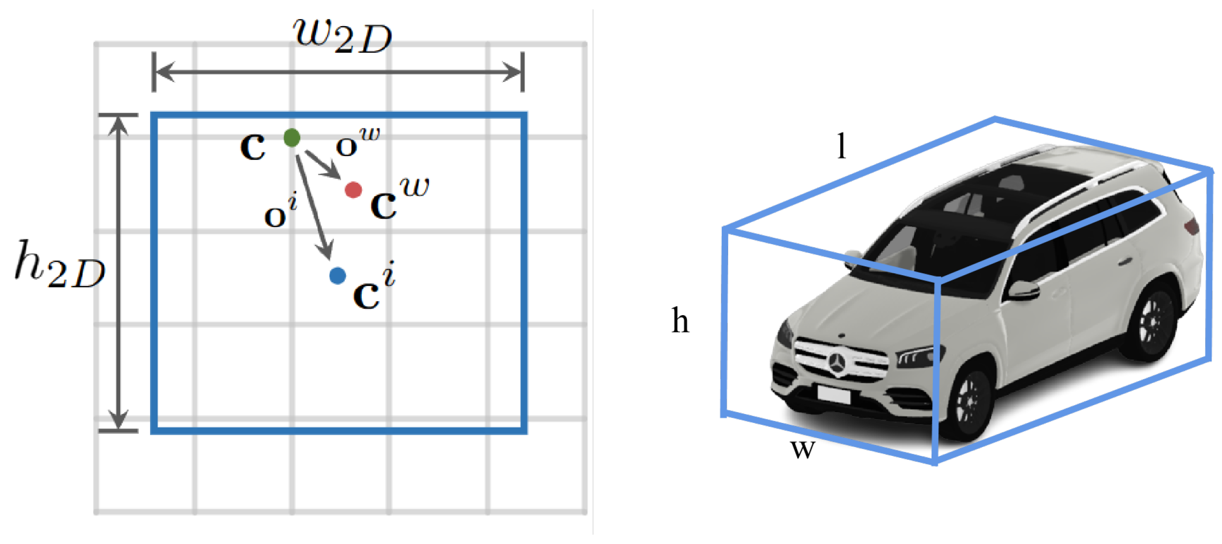
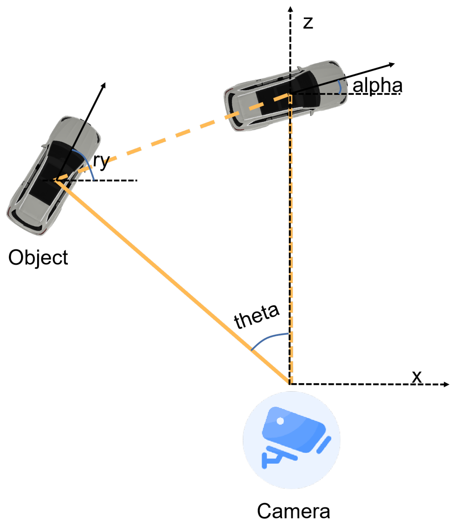
3.1. Task Description

In this work, we aim to detect 3D bounding boxes of vehicle objects in RGB images using the YOLOv7-3D model. Given an input image $I\in {\mathbb{R}}^{H\times W\times 3}$, camera intrinsic parameters $K\in {\mathbb{R}}^{3\times 3}$, and camera extrinsic parameters $P\in {\mathbb{R}}^{3\times 4}$, the output of the YOLOv7-3D model provides 3D bounding boxes for the traffic objects in the image, which can be represented as $B=\{B_1,B_2,\dots ,B_n\}$, where each bounding box $B_i$ consists of seven degrees of freedom:

$$B_i=\left(x_i,y_i,z_i,l_i,w_i,h_i,{\theta }_i\right)$$

(1)

Here, $(x,y,z)$ represents the position of the center point of each 3D bounding box in meters. $(l,w,h)$ denote the length, width, and height of the cuboid, respectively, in meters. $\theta$ represents the global orientation of each traffic object in space, which is the angle between the object’s heading direction and the x-axis of the camera coordinate system, in the range of $[-\pi ,\pi ]$.

The camera intrinsic parameters $K\in {\mathbb{R}}^{3\times 3}$ include parameters such as focal lengths, optical centers, and pixel sizes, which describe the optical characteristics and imaging process inside the camera. $f_u$ and $f_v$ are the focal lengths, while $c_u$ and $c_v$ represent the pixel coordinates of the optical center.

$$K=\left[\begin{array}{ccc}{f}_u& 0& c_u\\ 0& f_v& c_v\\ 0& 0& 1\end{array}\right]$$

(2)

The camera extrinsic parameters describe the camera’s position and orientation in the world coordinate system. It consists of the translation vector $T\in {\mathbb{R}}^{3\times 1}$ and the rotation matrix $R\in {\mathbb{R}}^{3\times 3}$, which map points in the camera coordinate system to the world coordinate system.

For a 3D point $X={[x,y,z]}^T$, it can be projected onto the image plane as $Y={[u,v,1]}^T$ using the camera projection matrix:

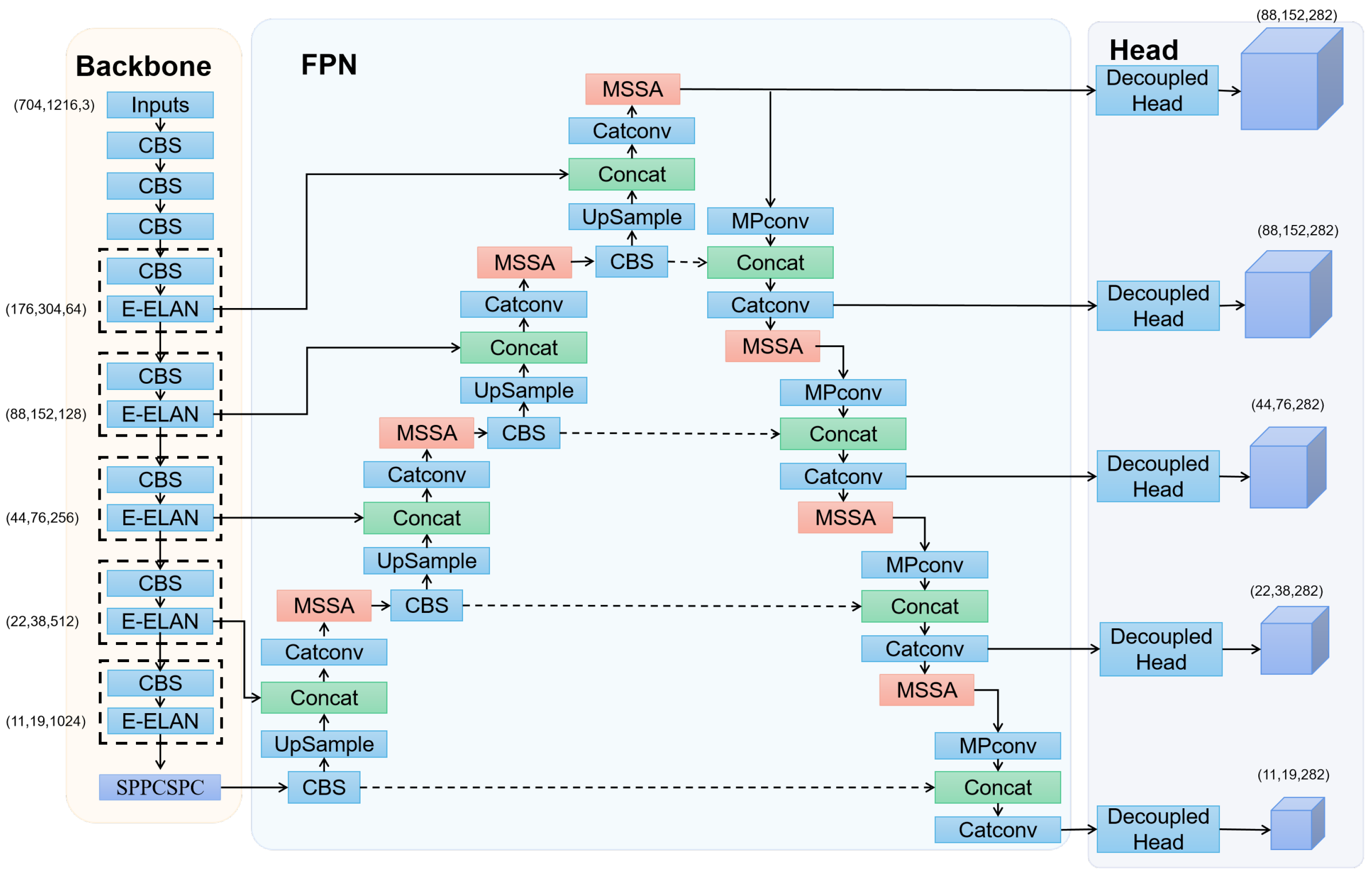
3.2. Model Structure

In terms of the model structure, YOLOv7-3D can be divided into three parts: the backbone feature extraction network, the multi-scale feature pyramid, and the multi-branch decoupled detection head. Due to the significant scale differences among various traffic objects in the Rope3D dataset, this paper proposes a 5-layer FPN structure and a multi-scale spatial attention mechanism (MSSA) to improve feature saliency and detection accuracy for different-scale objects. The overall network architecture of the model is shown in Figure 1.

In this work, the model does not directly predict the seven degrees of freedom of the targets $(x,y,z,l,w,h,\theta )$. Instead, it predicts nine degrees of freedom for the targets $(x_c,y_c,{\phi }_z,{\sigma }_z,l,w,h,sin\left(\theta \right),cos\left(\theta \right))$. Here, $x_c$ and $y_c$ represent the projected points of the center of the 3D bounding box on the 2D image. ${\phi }_z$ and ${\sigma }_z$ represent the depth value and the logarithmic variance of the depth value, respectively. The introduction of these parameters aims to quantify the uncertainty in the predictions by considering the variance. l, w, and h represent the length, width, and height of the 3D bounding box, respectively, while $sin\left(\theta \right)$ and $cos\left(\theta \right)$ are values required to compute the heading angle. The schematic diagram of degrees of freedom is shown in Figure 2.

3.2.1. Multi-Scale Feature Pyramids

The backbone network is primarily responsible for extracting features from the image and is structured as shown in the diagram. It consists of CBS convolutional layers, E-ELAN convolutional modules, MP-Conv convolutional modules, and SPPCSPC modules. The CBS convolutional layer comprises a convolutional layer, batch normalization layer (BN), and SiLU activation function, which are used to extract features at different scales. The E-ELAN convolutional module is an efficient aggregation network that modifies the calculation block while preserving the original transition layer structure. It enhances the network’s learning capacity without disrupting the original gradient paths through arithmetic techniques and allows the calculation blocks of different feature groups to learn more diverse features. The MP-Conv convolutional module combines the results of downsampling using max pooling and convolutional blocks, reducing computational complexity while increasing the receptive field and effectively propagating global information backward. The SPPCSPC module includes a spatial pyramid pooling layer that adapts to different resolutions using max pooling at four different scale sizes, distinguishing objects of different sizes.

In this paper, an additional layer, $P_6\in {\mathbb{R}}^{11\times 19\times 1024}$, is added to the original backbone feature network to detect large objects such as buses. Additionally, a larger-scale feature $P_2\in {\mathbb{R}}^{176\times 304\times 64}$ is utilized to detect smaller vehicle targets at a greater distance from the camera. Moreover, the channel numbers in the backbone feature extraction network are halved to avoid an excessive increase in parameters and computational complexity caused by increasing the depth of the model.

3.2.2. Multi-Scale Spatial Attention Mechanism

$$Y=K·\left[R\right|T]·X$$

(3)

FPN (Feature Pyramid Network) is a feature pyramid network used for multi-scale object detection. It constructs multi-scale feature maps by adding extra lateral connections in the Backbone network. These lateral connections extract features from different levels of the Backbone feature maps and merge them into the feature maps of the previous layer. This way, FPN can obtain rich semantic information at different scales and provide feature maps with different resolutions. This is crucial for detecting objects of different scales, as objects may have varying sizes and proportions. In this paper, the original 3-layer FPN structure in the YOLOv7 algorithm is modified to a 5-layer structure to accommodate more scale variations of the targets. As shown in the diagram, the upsampling structure of the FPN feature pyramid consists of CBS, UpSample, Concat, CatConv, and the multi-scale spatial attention mechanism.

Attention mechanisms are widely used to improve the performance of deep learning models by selectively focusing on relevant information and suppressing irrelevant or noisy information [38,39,40]. However, these attention mechanisms overlook the scale information of feature maps. This paper proposes a Multi-Scale Spatial Attention mechanism (MSSA), which adaptively adjusts the weights of features from P2 to P6. It increases the weights of scale features that are more beneficial for the recognition task while suppressing the weights of other scale features. Spatially, the model can focus on image textures and contextual information that are advantageous for the recognition task. The structure of MSSA is shown in the Figure 3. MSSA performs average pooling on the input 2D feature map $G\in {\mathbb{R}}^{C\times (H\times W)}$, with pooling kernel sizes of $K^h$ and $K^w$, and strides of $S^h$ and $S^w$ along the horizontal and vertical directions, respectively. This process generates condensed features $W_{\mathit{avg}}^c$ and $H_{\mathit{avg}}^c$. Subsequently, the features from these two condensed layers are aggregated:

(1) First, concatenate the compacted features. Since the dimensions of features $W_{\mathit{avg}}^c$ and $H_{\mathit{avg}}^c$ do not match, the width and height dimensions of feature $H_{\mathit{avg}}^c$ need to be transposed before concatenating it with $H_{\mathit{avg}}^c$ to obtain the feature map M.

(2) Second, set a hyperparameter r such that M is passed through a 2D convolution to obtain the feature map $M^1$, where the number of channels changes from c to $\frac{c}{r}$ In this paper, r is set, and the number of channels in $M^1$ should not be less than 8. Then, insert a BN layer and a SiLU activation function to obtain the feature map $M^2$. At this stage, $M^2$ incorporates both the feature compaction of the input feature G along the x-axis and y-axis, allowing spatial information of the input feature G to interact.

The mixed spatial information in $M^2$ is then divided, transposed, and passed through another 2D convolution to restore the channel number to c, resulting in $W^{\prime }$ and $H^{\prime }$. These two feature maps represent the spatial weights. Finally, element-wise multiplication is performed between $W^{\prime }$, $H^{\prime }$, and the corresponding elements of matrix G to obtain $G^{\prime }$. This process combines the spatial weights in the input feature map, where the spatial weights beneficial for the recognition task are increased. In the diagram, ⊙ represents element-wise multiplication between matrices. Thus, the spatial information S and channel information C are adaptively adjusted. This process can be represented as:

$$\begin{array}{cc}\hfill G^{\prime }& =\sigma (f\otimes (\left[AvgPoolW\right(\mathbf{G});AvgPoolH(\mathbf{G}\left)\right]\left)\right)\hfill \\ \hfill & =\sigma \left(f\otimes \left(\left[W_{\mathit{avg}}^c;H_{avg}^c\right]\right)\right)\hfill \end{array}$$

(4)

where $\sigma$ represents the sigmoid function, ⊗ represents the convolution process, and f is a convolution kernel.

Next, the feature map $G^{\prime }$ is adaptively average-pooled at scale L to obtain a compacted feature of size 2 × 1 × 1w. Then, an MLP is used to adjust the compacted feature, and a sigmoid function is applied to obtain the activated weights. Finally, the weights are added to the original feature map $G^{\prime }$ to obtain the feature map $G^{″}$. This process adapts the weights at scale L. It can be represented as:

$$\begin{array}{cc}\hfill G^{″}& =\sigma (f\otimes \left(\left[AvgPoolL\left({\mathbf{G}}^{\prime }\right)\right]\right))\hfill \\ \hfill & =\sigma (f\otimes \left(\left[W_{\mathit{avg}}^l\right]\right))\hfill \end{array}$$

(5)

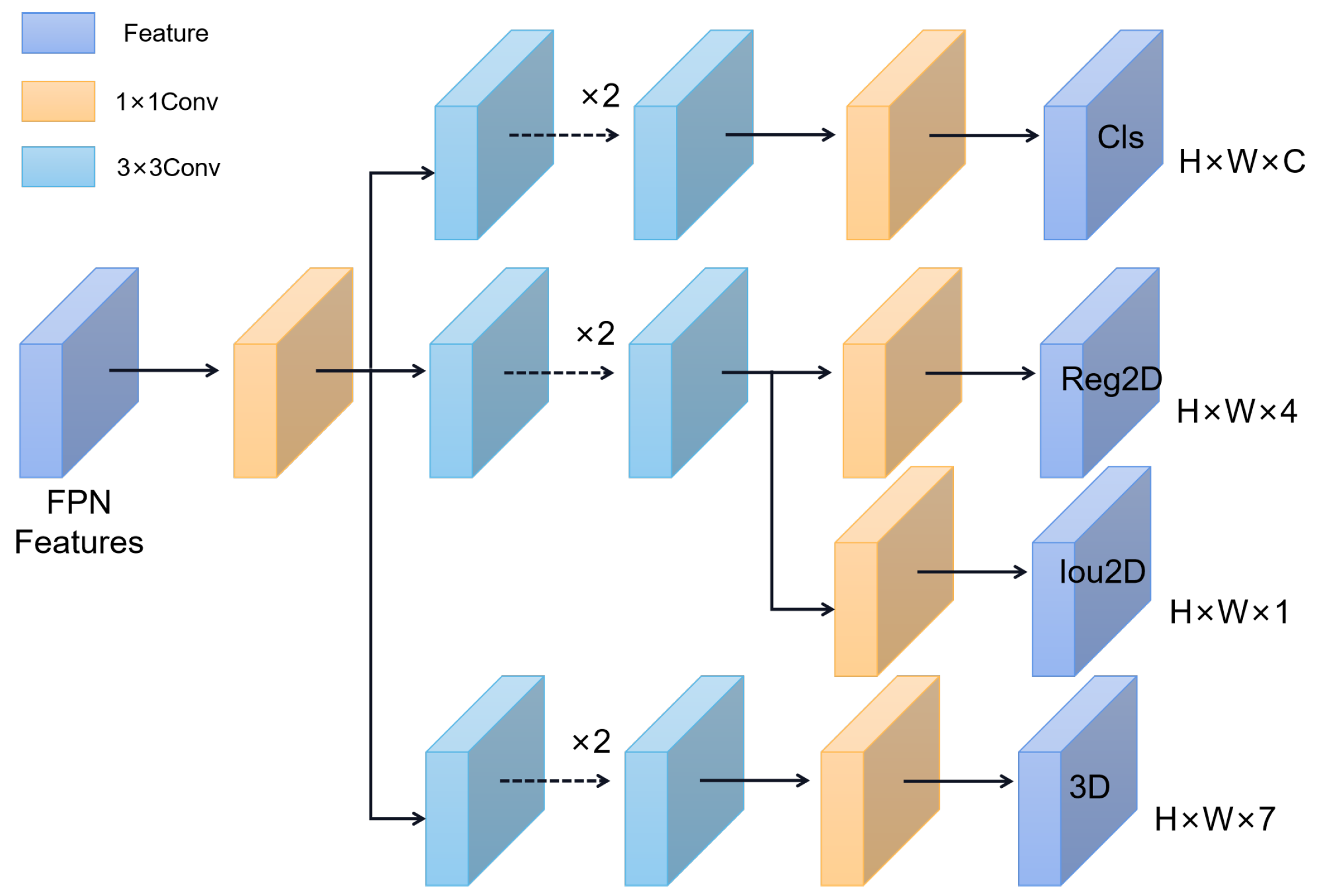
3.2.3. Multi-Branch Decoupling Detection Head

In object detection, the conflict between classification and regression tasks is a common problem. Therefore, the decoupling of classification and localization heads has been widely applied in both one-stage and two-stage detectors. However, despite the evolution of the YOLO series in terms of backbone and feature pyramid, its detection head remains coupled, as shown in Figure 4. In this paper, a multi-branch decoupled detection head is used in the detection stage. The model’s output includes predictions for 2D bounding box regression, object classification, projection of the 3D box’s center point $(x_c,y_c)$ onto the 2D image, depth value and logarithmic variance $({\phi }_z,{\sigma }_z)$ of the depth value, scale of the 3D box in terms of length, width, and height $(l,w,h)$, and the values required to compute the heading angle $sin\left(\theta \right)$ and $cos\left(\theta \right)$. The decoupled detection head consists of the following branches:

(1)

Reg2D(h, w, 4): Used to determine the regression parameters for each feature point, allowing adjustment of the predicted bounding boxes.

(2)

Obj(h, w, 1): Used to determine whether each feature point contains an object.

(3)

Cls(h, w, num classes): Used to determine the object class for each feature point.

(4)

CenterReg3D(h, w, 2): Used to determine the regression parameters for the 2D projection of the 3D object’s center point on the image.

(5)

Depth(h, w, 2): Used to determine the depth value and logarithmic variance for the 3D object.

(6)

Dim(h, w, 3): Used to determine the 3D dimensions (length, width, height) of the object.

(7)

Theta(h, w, 2): Used to determine the viewing angle of the 3D object.

Figure 4. Schematic diagram of Decoupled Head.

Figure 4. Schematic diagram of Decoupled Head.

Finally, the seven prediction results are stacked together. The results obtained for each feature layer are of size Out(h, w, 13 + 1 + num classes). The first four parameters are used to determine the 2D regression parameters for each feature point, allowing adjustment of the predicted bounding boxes. The fifth parameter is used to determine whether each feature point contains an object. Parameters six to thirteen are used to obtain the 9 degrees of freedom for the object in 3D space. Finally, the last num class parameters are used to determine the object class for each feature point.

3.3. Loss Function

In this work, the model does not directly predict the seven degrees of freedom of the object $(x,y,z,l,w,h,\theta )$ but predicts nine degrees of freedom $(x_c,y_c,{\phi }_z,{\sigma }_z,l,w,h,sin\left(\theta \right),cos\left(\theta \right))$. Here, $(x_c,y_c)$ represent the projected 2D coordinates of the center point of the 3D bounding box on the image. $({\phi }_z,{\sigma }_z)$ denote the depth compensation value and the logarithmic variance of the depth value. The introduction of ${\sigma }_z$ aims to quantify the uncertainty of the predictions by considering the variance. $(l,w,h)$ represent the length, width, and height of the 3D bounding box. $(sin(\theta ),cos(\theta \left)\right)$ are used to compute the heading angle.

Classification loss function: The paper introduces Focal Loss to address the issue of class imbalance in the Rope3D dataset. Focal Loss reduces the weight assigned to easily classified samples and increases the weight assigned to hard samples in order to focus more on challenging samples. This helps improve the performance of the model in scenarios with class imbalance:

$$L_{cls}=-{\alpha }_t{(1-P_t)}^{\gamma }log\left(P_t\right)$$

(6)

where $P_t$ is the predicted probability by the model, indicating the probability of the sample belonging to the target class. ${\alpha }_t$ is the balance factor used to adjust the weights of positive and negative samples. In general, it is defined as the ratio of the number of positive samples to the total number of samples. $\gamma$ is the focusing parameter used to adjust the weight difference between easily classified samples and hard samples. A larger value of $\gamma$ will make the model pay more attention to hard samples.

2D box regression loss function: For the prediction of the 2D bounding box, this paper uses the CIoU (Complete Intersection over Union) loss.

$$L_{IOU}=1-IOU+\frac{{\rho }^2\left(b,b^{*}\right)}{c^2}+\alpha v$$

(7)

where IOU represents the traditional Intersection over Union, ${\rho }^2(b,b^{*})$ denotes the Euclidean distance between the center points of the predicted box and the ground truth box. $\alpha$ is a balance factor used to adjust the weights of the position and shape losses, and v represents the position and shape loss. The specific formula is as follows:

$$\begin{array}{c}\alpha =\frac{v}{1-IOU+v}\\ v=\frac{4}{{\pi }^2}{\left(arctan\frac{w^{*}}{h^{*}}-arctan\frac{w}{h}\right)}^2\end{array}$$

(8)

Projection center point loss function: For the projection of the 3D object center point onto the 2D image, this paper uses L1 loss for direct regression. Unlike previous methods, this paper modifies the prediction of the center point to be an offset relative to the center point of the 2D bounding box rather than an offset relative to the entire image. Here, P represents the ground truth projected point coordinates, and $P^{*}$ represents the predicted projected point coordinates.

$$L_{center}={\left|\left|P-P^{*}\right|\right|}_1$$

(9)

Dimension-aware loss function: For the prediction of the 3D bounding box dimensions, this paper employs a dimension-aware L1 loss function that is suitable for size estimation. The loss function is defined as follows:

$$L_{dim}=\Vert \frac{\left(\mathbf{s}-{\mathbf{s}}^{*}\right)}{\mathbf{s}}{\Vert }_1$$

(10)

Here, $\Vert ·{\Vert }_1$ denotes the L1 norm. Previous algorithms used a baseline L1 loss, i.e., $L_{dim}^{\prime }=\Vert \mathbf{s}-{\mathbf{s}}^{*}{\Vert }_1$. It is worth noting that, compared to the baseline L1 loss $L_{dim}^{\prime }$, the dimension-aware loss used in this paper incorporates dynamic compensation generation. By re-computing $L_{dim}^{\prime }$, compensation weights $w_{dim}=L_{dim}^{\prime }/L_{dim}$ are generated to make the average value of the final loss function $L_{dim}$ equal to the standard loss. In this way, the proposed loss can be seen as a redistribution of the standard L1 loss.

Viewpoint loss function: Instead of directly predicting the object’s yaw angle (the global orientation angle of the object in the camera coordinate system, ranging from $-\pi$ to $\pi$), this paper chooses to regress the observation angle $\theta$ for each object. The observation angle $\theta$ represents the angle between the object’s direction and the camera axis, with the camera origin as the center and the line connecting the camera origin to the object’s center as the radius, after rotating the object around the camera’s y-axis to align with the camera’s z-axis. The transformation relationship between these two angles is shown in Figure 5. In addition, each is encoded as a vector. Using the target position, the yaw angle can be obtained: Furthermore, each $\theta$ is encoded as a vector ${\left[sin\left(\theta \right),cos\left(\theta \right)\right]}^T$. By using $\theta$ and the object’s position, the yaw angle $ry$ can be obtained:

$$\begin{array}{cc}\hfill ry+\frac{\pi }{2}-\theta & =\alpha +\frac{\pi }{2}\hfill \\ \hfill \alpha & =ry-\theta \hfill \end{array}$$

(11)

The final viewpoint loss function computes the loss using SmoothL1Loss on the normalized ${\left[sin\left(\theta \right),cos\left(\theta \right)\right]}^T$.

Depth loss function: In 3D object detection, depth estimation is a task with uncertainty since the depth of an object in real-world scenarios can be influenced by various factors such as viewpoint, occlusion, and image noise. This paper utilizes the Laplacian Aleatoric Uncertainty Loss to predict the depth of 3D objects, quantifying the uncertainty of the predictions by introducing a variance term. This loss reduces the weight of depth predictions with higher variance (i.e., greater uncertainty), thereby increasing the accuracy and reliability of depth predictions with lower uncertainty.

$$L_{depth}=\frac{1}{\left|\mathbb{P}\right|}\sum _{(x_c,y_c)\in \mathbb{P}}\frac{\sqrt{2}}{{\sigma }_z}\left|z-z^{*}\right|+log\left({\sigma }_z\right)$$

(12)

Here, $\mathbb{P}$ represents the set of real 2D bounding box centers, $({\phi }_z,{\sigma }_z)$ denotes the depth offset and logarithmic variance, z is the true depth value of the object, and $z^{*}$ is the predicted depth value of the object. The predicted depth value $z^{*}$ is obtained by reversing the sigmoid transformation of the model’s predicted depth offset ${\phi }_z$ back to the original linear range:

$$z^{*}=\frac{1}{sigmoid\left({\phi }_z\right)+ϵ}-1$$

(13)

By combining the projected points of the center on the feature map $(x_c,y_c)$, the inverse matrix of the camera intrinsic parameters $K^{-1}\in {\mathbb{R}}^{3\times 3}$, the 3D center position of the object in meters can be calculated as:

$${\left[\begin{array}{c}x\hfill \\ y\hfill \\ z\hfill \end{array}\right]}_{3D}=K_{3\times 3}^{-1}{\left[\begin{array}{c}z{x}_c\\ z{y}_c\\ z\end{array}\right]}_{2D}$$

(14)

Once the seven degrees of freedom for the 3D bounding box are obtained, the coordinates of the eight corners of the 3D box on the 2D image can be calculated as:

$$B=R_{\theta }\left[\begin{array}{c}\pm h/2\\ \pm w/2\\ \pm l/2\end{array}\right]+\left[\begin{array}{c}x\hfill \\ y\hfill \\ z\hfill \end{array}\right]$$

(15)

Here, $R_{\theta }$ is the rotation matrix for the yaw angle, ${[h,w,l]}^T$ represents the object’s 3D dimensions, and ${[x,y,z]}^T$ represents the object’s center coordinates.The overall loss is the sum of all the individual loss terms, with each loss term having a balancing weight parameter.

4. Experiments

In this section, the paper describes the details of model training and the effectiveness of data augmentation, conducts ablation experiments, and analyzes the experimental results. Additionally, in the last subsection, a quantitative comparison is made between YOLOv7-3D and some state-of-the-art monocular 3D object detection algorithms. The paper employed 4 NVIDIA GeForce RTX 3090 GPUs for training the model with a batch size of 4 and a total of 300 epochs. The SGD optimizer with betas $(0.9,0.009)$, an initial learning rate of 0.01, and a weight decay of 0.0005 was used.

4.1. Dataset

This paper uses the Rope3D dataset, which is based on roadside surveillance perspectives. This dataset has collected a total of 50,009 image frames under different times (day, night, dusk/dawn), different weather conditions (sunny, cloudy, rainy), different densities (crowded, normal, sparse), and different distributions of traffic elements, etc. It has the characteristics of being large-scale and multi-view. Some of its samples are shown in Figure 6. The dataset includes 13 object categories with their corresponding labels, 2D attributes (occlusion, truncation), and 7 degrees of freedom for 3D bounding boxes: position (x, y, z), dimensions (width W, length L, height H), and orientation (heading angle $\theta$). Additionally, the Rope3D dataset presents greater detection challenges due to significant occlusion, as shown in Figure 6. 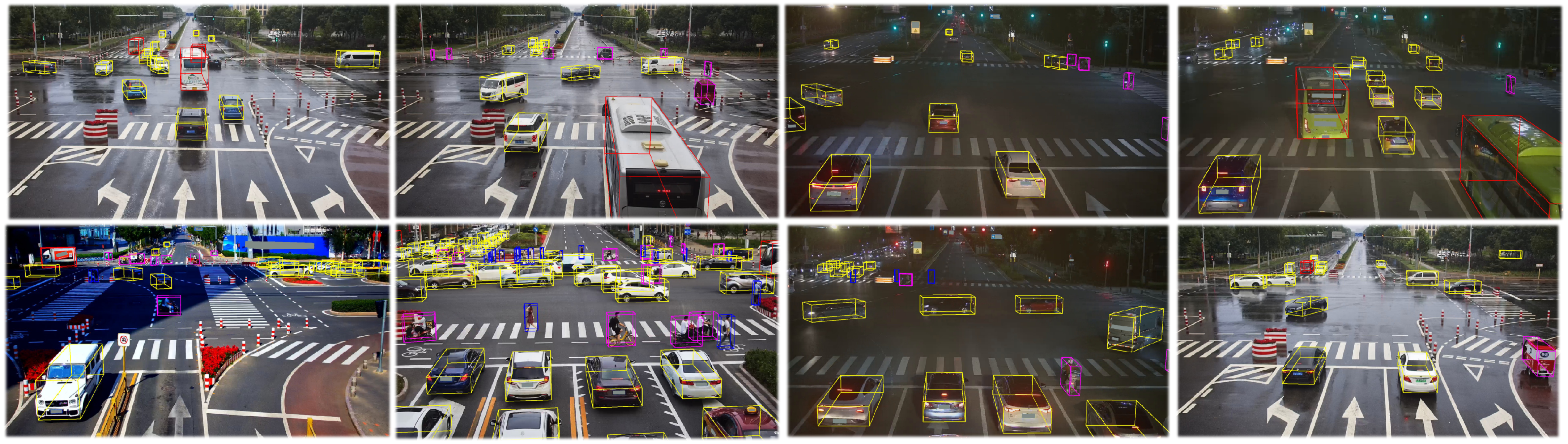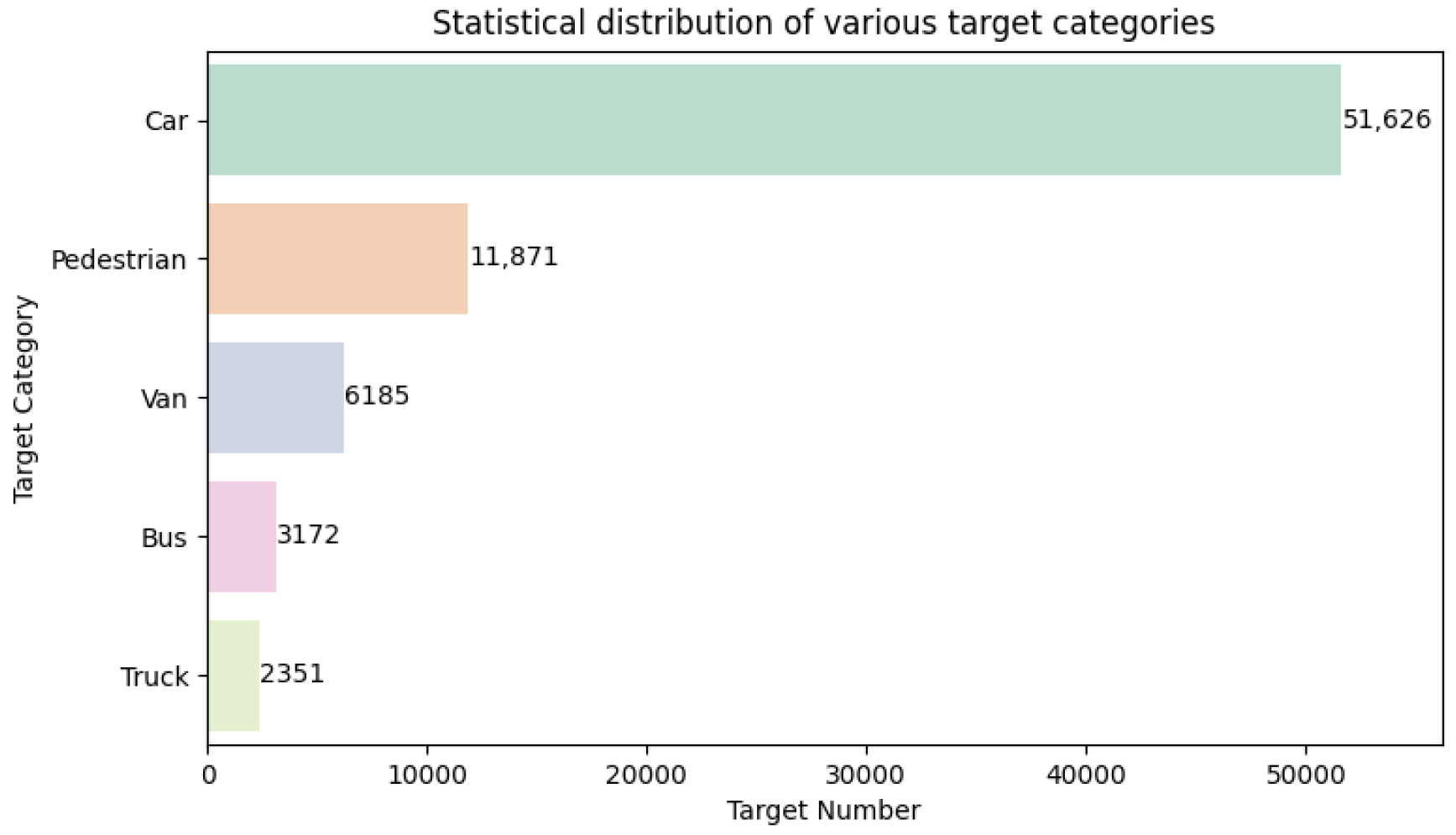Over half of the objects are partially or fully occluded, whereas the occlusion percentage in the KITTI dataset [41] ranges from 5% to 30%. This highlights the increased difficulty of detection in the Rope3D dataset.

Additionally, this paper conducted a statistical analysis of the distribution of different object categories in the training and validation sets of the Rope3D dataset, as shown in Figure 7. It was found that there is a significant class imbalance in the dataset. To address this issue and improve the classification accuracy, the study introduced the Focal Loss technique.

Furthermore, this study employed the K-means++ algorithm to cluster the sizes of the target objects in the Rope3D dataset into several clusters, with each cluster’s centroid size serving as the prior box size. As shown in Figure 8, there is a significant variation in size within each cluster and distinct scale differences and boundaries between clusters. This observation reflects the substantial diversity in object scales within the dataset. Therefore, this study designed a 5-layer Feature Pyramid Network (FPN) architecture and a multi-scale spatial attention mechanism.

4.2. Real-Time Data Augmentation

Data augmentation is a common technique in 2D object detection to increase training data diversity and enrich the model’s robustness and generalization capabilities. In this paper, the commonly used 2D data augmentation methods were adapted to 3D object detection. Random scaling, translation, horizontal flipping, color transformations, and brightness adjustments were implemented for 3D objects. The scaling range was set from 0.75 to 2. The results, as shown in Figure 9, present the 2D bounding boxes in green, the 3D bounding boxes in white, black dots representing the center of the 2D boxes, red dots representing the center of the 3D boxes, and green dots representing the center of the bottom face of the 3D boxes. The gaps resulting from scaling were filled with gray pixels.

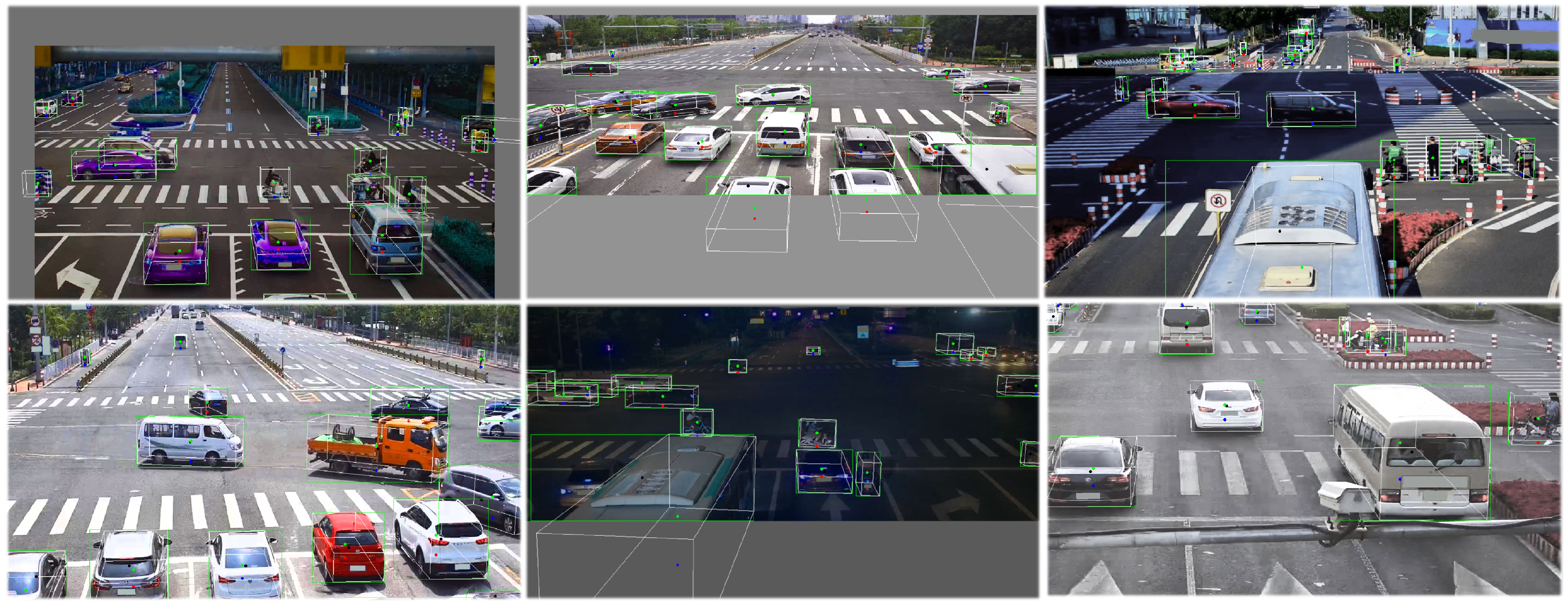
4.3. Experiments and Analysis

In the experiments, this paper primarily compared its approach with the following monocular visual 3D object detection algorithms: (1) KM3D, which employed ResNet34 as the backbone network. (2) Kinematic3D, a video-based monocular 3D object detector utilizing DenseNet121 as the backbone network. (3) MonoDLE, a center-point-based single-stage detector based on CenterNet, employing DLA34 as the backbone network.

In the experimental setup, “Ours Base” represents the improved baseline model of YOLOv7 capable of simultaneously detecting 2D and 3D objects. “Ours +5Head” indicates the model with five detection heads built upon the base model. “Ours +MSSA” signifies the YOLOv7-3D model incorporating the multi-scale spatial attention mechanism on top of the previous model.

The comparison of the experimental and ablation study results is shown in

Table 1. The comparison of the experimental and ablation study.

Method	Backbone	AP3D/IoU = 0.5								Params (M)	GFlops
		Car	Van	Bus	Truck	Cyclist	Motorcyclist	Tricyclist	Pedestrian
KM3D	ResNet34	8.97	7.77	3.97	4.94	11.81	11.35	10.39	12.61	26.881	422.276
Kinematic3D	DenseNet121	11.42	10.65	4.02	4.83	11.35	15.08	11.24	14.43	25.913	296.441
MonoDLE	DLA34	12.84	11.21	4.19	5.25	13.23	16.58	11.72	14.75	20.310	264.898
Ours Base	CSPDarknet	11.75	10.98	1.86	4.50	14.24	17.46	11.03	13.19	37.626	222.563
Ours+5Head	CSPDarknet	12.25	10.73	1.78	3.68	15.45	18.73	11.66	14.83	42.235	87.625
Ours + MSSA	CSPDarknet	13.02	11.33	2.44	4.53	15.69	19.13	11.77	14.81	42.957	88.453

. The analysis of experimental results reveals that KM3D achieved lower average precision across all categories. It performed relatively well in the Cyclist and Motorcyclist categories but poorly in the Bus and Truck categories. Kinematic3D, on the other hand, obtained higher average precision compared to KM3D across all categories. It performed well in the Cyclist, Motorcyclist, and Pedestrian categories but poorly in the Van and Bus categories. MonoDLE achieved higher average precision than KM3D and Kinematic3D across all categories. It performed well in the Cyclist, Motorcyclist, and Pedestrian categories. Ours Base showed poor performance in the Car, Van, and Bus categories but relatively good performance in the Cyclist, Motorcyclist, and Pedestrian categories. Adding five detection heads to the Base model resulted in higher average precision across all categories compared to Ours Base. It performed well in the Cyclist, Motorcyclist, and Pedestrian categories. Finally, incorporating MSSA resulted in the highest average precision across all categories. It performed best in the Cyclist, Motorcyclist, and Pedestrian categories. Overall, based on the given experimental data, the Ours + MSSA method achieved the best average precision across multiple categories. Additionally, categories such as Bus achieved lower precision compared to the aforementioned methods due to the imbalance in the dataset, where the Bus and Truck categories have a very small number of instances, resulting in less training exposure for the model to learn other categories effectively.

The model’s parameter count and computational load are crucial metrics for assessing algorithm detection speed. The results indicate that Ours Base has a relatively large parameter count compared to other models. However, by modifying it to incorporate five detection heads and halving the main channel count, the model’s parameters increased from 37M to 42M. Notably, the computational load decreased significantly from 222G to 87G, accompanied by improvements in the supervised accuracy for various categories. In contrast, Ours + MSSA showed only a slight increase in parameter count yet achieved enhanced detection accuracy for different target categories. This suggests that Ours + MSSA improves model performance without introducing a substantial number of redundant parameters and computational burden. Considering accuracy, model parameter count, and computational load comprehensively, Ours + MSSA demonstrates outstanding performance in traffic object detection tasks. The method enhances detection accuracy while maintaining a relatively modest model complexity, showcasing excellent practicality.

4.4. Detection Performance in Different Ranges

To further analyze the performance of the models in different distance ranges, this study employed the Score metric, which encompasses the following components: ACS (Average Center Score): This represents the average score of the object’s center point. It is calculated based on the distance or similarity between the estimated center point and the ground truth center point. ACS is used to evaluate the accuracy of the object detection algorithm in estimating the object’s center point.

$$ACS=\frac{1}{\left|D\right|}\sum _{s\in D}\left(1-min\left(1,\frac{{\Delta }_s^c}{C_s}\right)\right)$$

(16)

D represents the set of true positive samples, $C_s$ is the norm of the ground truth center, and $\Delta {}_s^c$ is the Euclidean distance between the predicted ground center and the ground truth center for sample s. $\left|D\right|$ is the total number of true positive objects. AOS (Average Overlap Score): It represents the average overlap score of the object bounding boxes. It is computed by measuring the overlap between the detected bounding boxes and the ground truth bounding boxes. AOS is used to evaluate the accuracy of object localization.

$$AAS=\frac{1}{\left|D\right|}\sum _{s\in D}\left(1-min\left(1,\frac{{\Delta }_s^A}{A_s}\right)\right)$$

(17)

$\Delta {}_s^{\theta }$ represents the angular difference for sample s, and $cos\left(2\ast \Delta {}_s^{\theta }\right)$ accounts for the fact that during evaluation, no distinction is made between whether the head or tail of an object is facing the camera. ASS (Average Size Score): It represents the average score for object size. It is calculated by measuring the size difference between the detected bounding boxes and the ground truth bounding boxes. $\Delta {}_s^A$ is the absolute area difference, and $A_s$ is the ground truth area. ASS evaluates the accuracy of object size estimation.

$$AOS=\frac{1}{\left|D\right|}\sum _{s\in D}\frac{1+cos\left(2\ast {\Delta }_s^{\theta }\right)}{2}$$

(18)

AGS (Average Four Ground Points Distance and Similarity): This represents the average geometric distance score (relative value) for object shape. It is calculated by measuring the geometric distance between the detected shape and the ground truth shape of the object. $\widehat{s_g}$ and $s_g$ represent the g-th predicted point and the g-th ground truth point for sample s, respectively. K = 4 denotes the total number of ground truth points.

$$AGS=\frac{1}{\left|D\right|}\sum _{s\in D}\left(1-min\left(1,\frac{1}{K}\sum _{g=0}^{K-1}\frac{\left|s_g-\widehat{s_g}\right|}{|\widehat{c}|}\right)\right)$$

(19)

(ACS + AOS + ASS + AGS)/4.0: It represents the overall score, which is the average of the four mentioned scores. This overall score can be used to comprehensively evaluate the performance of the object detection algorithm.

As shown in

Table 2. The comparison results of detection performance in different distance ranges.

Method	Range (m)	Score
		Car	Big Vehicle	Cyclist	Pedestrian
MonoDLE	all	92.8	86.3	88.5	92.2
	0–30	89.8	84.0	87.1	92.0
	30–60	91.7	85.3	88.7	92.7
	60–90	92.7	90.9	88.9	91.9
	90–120	92.89	89.3	86.2	91.3
Ours	all	94.4	89.7	89.1	91.9
	0–30	92.8	86.9	88.5	91.8
	30–60	94.7	92.0	89.3	92.5
	60–90	94.5	91.9	88.6	92.4
	90–120	93.7	90.0	88.8	90.9

, the model achieves high detection accuracy in the mid-range distances, particularly within the range of 30–60 m. However, the detection accuracy is lower in the range of 90–120 m. This can be attributed to two reasons: the region with strong features for learning in the image is too small, and there is a significant reduction in 3D annotations due to occlusion in distant regions. MonoDLE performs well in pedestrian detection, while the proposed algorithm in this paper shows significant improvement in Car, Big Vehicle, and Cyclist categories.

5. Conclusions

The paper proposes a method called YOLOv7-3D for single-camera 3D traffic object detection in roadside monitoring scenarios. Through experiments and evaluations on the Rope3D dataset, our YOLOv7-3D algorithm achieves significant performance results in single-camera 3D traffic object detection. Compared to traditional methods based on 2D image processing, our algorithm accurately captures the position, size, and orientation information of traffic objects, as well as estimates the distance between vehicles and the camera. By overcoming the limitations and challenges of a single-camera perspective, our algorithm enables more accurate and reliable traffic object detection, providing a more reliable guarantee for urban traffic safety and efficiency. Future research directions include further optimizing algorithm performance and exploring integration with other traffic monitoring systems to achieve more intelligent and efficient traffic management and control.

References

- Cui, J.; Qiu, H.; Chen, D.; Stone, P.; Zhu, Y. Coopernaut: End-to-end driving with cooperative perception for networked vehicles. In Proceedings of the IEEE/CVF Conference on Computer Vision and Pattern Recognition, New Orleans, LA, USA, 19–24 July 2022; pp. 17252–17262. [Google Scholar]
- Huang, J.; Huang, G.; Zhu, Z.; Ye, Y.; Du, D. Bevdet: High-performance multi-camera 3d object detection in bird-eye-view. arXiv 2021, arXiv:2112.11790. [Google Scholar]
- Yu, H.; Luo, Y.; Shu, M.; Huo, Y.; Yang, Z.; Shi, Y.; Guo, Z.; Li, H.; Hu, X.; Yuan, J.; et al. Dair-v2x: A large-scale dataset for vehicle-infrastructure cooperative 3d object detection. In Proceedings of the IEEE/CVF Conference on Computer Vision and Pattern Recognition, New Orleans, LA, USA, 19–24 July 2022; pp. 21361–21370. [Google Scholar]
- Xu, R.; Xiang, H.; Tu, Z.; Xia, X.; Yang, M.H.; Ma, J. V2x-vit: Vehicle-to-everything cooperative perception with vision transformer. In European Conference on Computer Vision; Springer: Berlin/Heidelberg, Germany, 2022; pp. 107–124. [Google Scholar]
- Adaimi, G.; Kreiss, S.; Alahi, A. Deep Visual Re-identification with Confidence. Transp. Res. Part C Emerg. Technol. 2021, 126, 103067. [Google Scholar] [CrossRef]
- Ghahremannezhad, H.; Shi, H.; Liu, C. Real-Time Accident Detection in Traffic Surveillance Using Deep Learning. In Proceedings of the 2022 IEEE International Conference on Imaging Systems and Techniques (IST), Kaohsiung, Taiwan, 21–23 June 2022; IEEE: Piscataway, NJ, USA, 2022; pp. 1–6. [Google Scholar]
- Hu, Z.; Lam, W.H.; Wong, S.C.; Chow, A.H.; Ma, W. Turning traffic surveillance cameras into intelligent sensors for traffic density estimation. Complex Intell. Syst. 2023, 1–25. [Google Scholar] [CrossRef]
- Naphade, M.; Wang, S.; Anastasiu, D.C.; Tang, Z.; Chang, M.C.; Yao, Y.; Zheng, L.; Rahman, M.S.; Arya, M.S.; Sharma, A.; et al. The 7th AI City Challenge. In Proceedings of the IEEE/CVF Conference on Computer Vision and Pattern Recognition, Vancouver, BC, Canada, 18–22 June 2023; IEEE: Piscataway, NJ, USA, 2023; pp. 5537–5547. [Google Scholar]
- Fernandez-Sanjurjo, M.; Bosquet, B.; Mucientes, M.; Brea, V.M. Real-Time Visual Detection and Tracking System for Traffic Monitoring; Elsevier: Amsterdam, The Netherlands, 2019; Volume 85, pp. 410–420. [Google Scholar]
- Zhang, C.; Ren, K. LRATD: A Lightweight Real-Time Abnormal Trajectory Detection Approach for Road Traffic Surveillance; Springer: Berlin/Heidelberg, Germany, 2022; Volume 34, pp. 22417–22434. [Google Scholar]
- Ghahremannezhad, H.; Shi, H.; Liu, C. Object Detection in Traffic Videos: A Survey. IEEE Trans. Intell. Transp. Syst. 2023, 24, 6780–6799. [Google Scholar] [CrossRef]
- Bochkovskiy, A.; Wang, C.Y.; Liao, H.Y.M. Yolov4: Optimal speed and accuracy of object detection. arXiv 2020, arXiv:2112.11790. [Google Scholar]
- Wang, C.Y.; Bochkovskiy, A.; Liao, H.Y.M. YOLOv7: Trainable bag-of-freebies sets new state-of-the-art for real-time object detectors. In Proceedings of the IEEE/CVF Conference on Computer Vision and Pattern Recognition, Vancouver, BC, Canada, 18–22 June 2023; pp. 7464–7475. [Google Scholar]
- Ye, X.; Shu, M.; Li, H.; Shi, Y.; Li, Y.; Wang, G.; Tan, X.; Ding, E. Rope3d: The roadside perception dataset for autonomous driving and monocular 3d object detection task. In Proceedings of the IEEE/CVF Conference on Computer Vision and Pattern Recognition, New Orleans, LA, USA, 19–24 July 2022; pp. 21341–21350. [Google Scholar]
- Yang, L.; Yu, K.; Tang, T.; Li, J.; Yuan, K.; Wang, L.; Zhang, X.; Chen, P. BEVHeight: A Robust Framework for Vision-based Roadside 3D Object Detection. In Proceedings of the IEEE/CVF Conference on Computer Vision and Pattern Recognition, Vancouver, BC, Canada, 18–22 June 2023; pp. 21611–21620. [Google Scholar]
- Hosseiny, A.; Jahanirad, H. Hardware acceleration of YOLOv7-tiny using high-level synthesis tools. Real-Time Image Proc. 2023, 20, 75. [Google Scholar] [CrossRef]
- Chen, H.; Huang, Y.; Tian, W.; Gao, Z.; Xiong, L. Monorun: Monocular 3d object detection by reconstruction and uncertainty propagation. In Proceedings of the IEEE/CVF Conference on Computer Vision and Pattern Recognition, Nashville, TN, USA, 20–25 June 2021; pp. 10379–10388. [Google Scholar]
- Ding, M.; Huo, Y.; Yi, H.; Wang, Z.; Shi, J.; Lu, Z.; Luo, P. Learning Depth-Guided Convolutions for Monocular 3D Object Detection. In Proceedings of the 2020 IEEE/CVF Conference on Computer Vision and Pattern Recognition Workshops (CVPRW), Seattle, WA, USA, 14–19 June 2020. [Google Scholar]
- Reading, C.; Harakeh, A.; Chae, J.; Waslander, S.L. Categorical Depth Distribution Network for Monocular 3D Object Detection. In Proceedings of the 2021 IEEE/CVF Conference on Computer Vision and Pattern Recognition (CVPR), Virtual, 19–25 June 2021. [Google Scholar]
- Wang, L.; Du, L.; Ye, X.; Fu, Y.; Guo, G.; Xue, X.; Feng, J.; Zhang, L. Depth-conditioned Dynamic Message Propagation for Monocular 3D Object Detection. In Proceedings of the 2021 IEEE/CVF Conference on Computer Vision and Pattern Recognition (CVPR), Virtual, 19–25 June 2021. [Google Scholar]
- Wang, Y.; Chao, W.L.; Garg, D.; Hariharan, B.; Campbell, M.; Weinberger, K.Q. Pseudo-lidar from visual depth estimation: Bridging the gap in 3D object detection for autonomous driving. In Proceedings of the IEEE/CVF Conference on Computer Vision and Pattern Recognition, Long Beach, CA, USA, 16–20 June 2019; IEEE: Piscataway, NJ, USA, 2019; pp. 8445–8453. [Google Scholar]
- Carrillo, J.; Waslander, S. Urbannet: Leveraging urban maps for long range 3D object detection. In Proceedings of the 2021 IEEE International Intelligent Transportation Systems Conference (ITSC), Indianapolis, IN, USA, 19–22 September 2021; IEEE: Piscataway, NJ, USA, 2021; pp. 3799–3806. [Google Scholar]
- Weng, X.; Kitani, K. Monocular 3D Object Detection with Pseudo-LiDAR Point Cloud. In Proceedings of the 2019 IEEE/CVF International Conference on Computer Vision Workshop (ICCVW), Seoul, Republic of Korea, 27 October–2 November 2019; IEEE: Piscataway, NJ, USA, 2019; pp. 857–866. [Google Scholar]
- Mousavian, A.; Anguelov, D.; Flynn, J.; Kosecka, J. 3D bounding box estimation using deep learning and geometry. In Proceedings of the IEEE conference on Computer Vision and Pattern Recognition, Honolulu, HI, USA, 21–26 July 2017; IEEE: Piscataway, NJ, USA, 2017; pp. 7074–7082. [Google Scholar]
- Ma, X.; Liu, S.; Xia, Z.; Zhang, H.; Zeng, X.; Ouyang, W. Rethinking pseudo-lidar representation. In Computer Vision–ECCV 2020, Proceedings of the 16th European Conference, Glasgow, UK, 23–28 August 2020; Springer: Berlin/Heidelberg, Germany, 2020; pp. 311–327. [Google Scholar]
- Ye, X.; Du, L.; Shi, Y.; Li, Y.; Tan, X.; Feng, J.; Ding, E.; Wen, S. Monocular 3D Object Detection via Feature Domain Adaptation. In Proceedings of the Computer Vision—ECCV 2020, Glasgow, UK, 23–28 August 2020; pp. 17–34. [Google Scholar]
- Brazil, G.; Liu, X. M3D-RPN: Monocular 3D Region Proposal Network for Object Detection. In Proceedings of the 2019 IEEE/CVF International Conference on Computer Vision (ICCV), Seoul, Republic of Korea, 27 October–2 November.
- Ma, X.; Zhang, Y.; Xu, D.; Zhou, D.; Yi, S.; Li, H.; Ouyang, W. Delving into localization errors for monocular 3D object detection. In Proceedings of the IEEE/CVF Conference on Computer Vision and Pattern Recognition, Virtual, 19–25 June 2021; IEEE: Piscataway, NJ, USA, 2021; pp. 4721–4730. [Google Scholar]
- Liu, X.; Xue, N.; Wu, T. Learning Auxiliary Monocular Contexts Helps Monocular 3D Object Detection. AAAI Proc. Aaai Conf. Artif. Intell. 2022, 36, 1810–1818. [Google Scholar] [CrossRef]
- Zhang, Y.; Lu, J.; Zhou, J. Objects are Different: Flexible Monocular 3D Object Detection. In Proceedings of the 2021 IEEE/CVF Conference on Computer Vision and Pattern Recognition (CVPR), Virtual, 19–25 June 2021. [Google Scholar]
- Zhou, X.; Koltun, V.; Krähenbühl, P. Tracking objects as points. In European Conference on Computer Vision; Springer: Berlin/Heidelberg, Germany, 2020; pp. 474–490. [Google Scholar]
- Simonelli, A.; Bulo, S.R.; Porzi, L.; López-Antequera, M.; Kontschieder, P. Disentangling monocular 3D object detection. In Proceedings of the IEEE/CVF International Conference on Computer Vision, Seoul, Republic of Korea, 27 October–2 November 2019; IEEE: Piscataway, NJ, USA, 2019; pp. 1991–1999. [Google Scholar]
- Liu, Z.; Wu, Z.; Tóth, R. Smoke: Single-stage monocular 3D object detection via keypoint estimation. In Proceedings of the IEEE/CVF Conference on Computer Vision and Pattern Recognition Workshops, Seattle, WA, USA, 13–19 June 2020; IEEE: Piscataway, NJ, USA, 2020; pp. 996–997. [Google Scholar]
- Zhou, X.; Karpur, A.; Gan, C.; Luo, L.; Huang, Q. Unsupervised domain adaptation for 3D keypoint estimation via view consistency. In Proceedings of the European Conference on Computer Vision (ECCV); Springer: Berlin/Heidelberg, Germany, 2018; pp. 137–153. [Google Scholar]
- Li, Z.; Chen, Z.; Li, A.; Fang, L.; Jiang, Q.; Liu, X.; Jiang, J. Unsupervised domain adaptation for monocular 3D object detection via self-training. In European Conference on Computer Vision; Springer: Cham, Switzerland, 2022; pp. 245–262. [Google Scholar]
- Adam, M.G.; Piccolrovazzi, M.; Eger, S.; Steinbach, E. Bounding box disparity: 3D metrics for object detection with full degree of freedom. In Proceedings of the 2022 IEEE International Conference on Image Processing (ICIP), Bordeaux, France, 16–19 October 2022; IEEE: Piscataway, NJ, USA, 2022; pp. 1491–1495. [Google Scholar]
- Li, P.; Zhao, H.; Liu, P.; Cao, F. RTM3D: Real-time Monocular 3D Detection from Object Keypoints for Autonomous Driving. In Proceedings of the Computer Vision—ECCV 2020, Glasgow, UK, 23–28 August 2020; pp. 644–660. [Google Scholar]
- Hu, J.; Shen, L.; Albanie, S.; Sun, G.; Wu, E. Squeeze-and-Excitation Networks. In Proceedings of the 2018 IEEE/CVF Conference on Computer Vision and Pattern Recognition (CVPR), Salt Lake City, UT, USA, 18–22 June 2018; pp. 7132–7141. [Google Scholar]
- Woo, S.; Park, J.; Lee, J.Y.; Kweon, I.S. CBAM: Convolutional Block Attention Module. In Proceedings of the Computer Vision—ECCV 2018, Munich, Germany, 8–14 September 2018; pp. 3–19. [Google Scholar]
- Hou, Q.; Zhou, D.; Feng, J. Coordinate Attention for Efficient Mobile Network Design. In Proceedings of the 2021 IEEE/CVF Conference on Computer Vision and Pattern Recognition (CVPR), Nashville, TN, USA, 20–25 June 2021. [Google Scholar]
- Geiger, A.; Lenz, P.; Stiller, C.; Urtasun, R. Vision Meets Robotics: The Kitti Dataset; Sage Publications: London, UK, 2013; Volume 32, pp. 1231–1237. [Google Scholar]