Numerical Study of the Flow and Blockage Ratio of Cylindrical Pier Local Scour

Abstract

A three-dimensional large eddy simulation model is used to simulate the turbulent flow dynamics around a circular pier in live-bed and clear-water scour conditions. The Navier–Stokes equations are transformed into a $\sigma$-coordinate system and solved using a second-order unstructured triangular finite-volume method. We simulate the bed evolution by solving the Exner-Polya equation assisted by a sand-slide model as a correction method. The bedload transport rate is based on the model of Engelund and Fredsœ. The model was validated for live-bed conditions in a wide channel and clear-water conditions in a narrow channel against the experimental data found in the literature. The in-house model NSMP3D can successfully produce both the live-bed and clear-water scouring throughout a stable long-term simulation. The flow model was used to study the effects of the blockage ratio in the flow near the pier in clear-water conditions, particularly the contraction effect at the zone where the scour hole starts to form. The scour depth in the clear water simulations is generally deeper than the live-bed simulations. In clear-water, the results show that the present model is able to qualitatively and quantitatively capture the hydrodynamic and morphodynamic processes near the bed. In comparison to the wide channel situation, the simulations indicate that the scour rate is faster in the narrow channel case.

1. Introduction

Scour erosion refers to an increase in local sediment transport at the base of a submerged structure due to the vortices generated by fluid–structure interactions. According to Raudkivi and Ettema, 1983 [1], scour in rivers can be classified into three categories:

(i)

General scour, which occurs irrespective of the presence of an obstacle.

(ii)

Contraction scour, which occurs as a result of constriction due to lateral groins, spur dikes, or bridge abutments.

(iii)

Local scour, which is only observed at the base of the obstacle and does not lead to sediment transport far from the pier.

Raudkivi and Ettema, 1983 [1], distinguish the first and last types as live-bed scour and clear-water scour, respectively. The shear stress exerted by the approaching flow determines the type of scour at the base of a structure. Clear-water scour occurs as a result of inflow shear stresses which are less than or equal to the threshold for sediment motion, whereas live-bed scour occurs for inflow shear stresses that are greater than this threshold (Melville et al., 1999 [2]). In the literature, this threshold between clear-water and live-bed conditions has been described in a number of ways. Ettema et al., 2017 [3], expressed it as the mean velocity needed for the entrainment of the bed, while Roulund et al., 2005 [4], expressed it as a critical value for the Shields number associated with the friction velocity, $u_{\tau }$.

Examples of clear-water conditions can be found in nature, such as at the Tahrir and Imbaba bridges in Cairo, Egypt (Stevens et al., 1991 [5]), and also in laboratory studies (Williams et al., 2018 [6]). Scouring at the base of bridge piers has been found to be the third global cause of bridge collapse (Proske, 2018 [7]) after impact and flooding. However, the leading causes of bridge collapse vary significantly in dependence with the geographical situation, construction and inspection standards (Arneson et al., 2012 [8]). As a result, some regional studies have found that bridge scouring is responsible for between 50% and 64% of bridge failures [9,10,11,12]. This problem highlights the importance of studying the scouring process; hence, there is interest in numerical models capable of accurately modeling this case.

The characteristics of the flow around a cylindrical pier are well known, and the turbulent structures present have been extensively described in the past [4,13,14,15]. Upstream from the cylinder, the main structure responsible for scouring is a horseshoe vortex (HSV) system. This is also the case downstream in live-bed conditions, but in clear-water conditions, the HSV competes against wake vortices (WV) in the deposition and scouring processes (Lachaussée et al., 2018 [16]). However, despite the many existing studies on pier scouring, our current understanding of this process remains incomplete. A recent study by Lai et al., 2022 [17], pointed out that the gap between the numerical predictions of equilibrium scouring and experimental results can be traced to the limitations of the current sediment transport theory. As Lachaussée, 2018 [18], observed, there is a noteworthy disparity between studies of live-bed scouring [4,19,20,21,22,23,24,25] and clear-water scouring [26,27,28,29], the latter being much less studied.

There are many empirical and semi-empirical formulae for predicting bedload transport available in the literature (VanRijn, 1993 [30], but their predictions differ in certain regimes. Most sediment models need a sand-slide model to control the angles of scouring and deposition (Zhang, 2019 [31]). In clear-water conditions, the majority of models consider the bed load [27,28,29], although the suspended load has been considered for flow velocities in the upper spectrum (Olsen and Melaaen, 1993 [26]. The usual approaches for turbulence modeling include RANS [26,27] and URANS (Khosronejad et al., 2012 [28]) approaches. The scour equilibrium depth at the upstream face of the cylinder is frequently reported in studies, while the dune downstream and the kinematics of scour hole evolution are rarely described (Lai et al., 2022 [17]). Furthermore, while a few studies have been performed in computational domains that could be considered narrow channels [26,28], the effects of the channel width on sediment transport tend to be dismissed. This is because the traditional approach seeks to emulate an open channel by using virtual lateral walls boundaries.

In a fluid–structure problem tested between two lateral walls, the term “narrow channel” is used when the lateral walls affect the flow pattern in the vicinity of the structure and at its wake. A number of conditions will determine whether the wall effect is negligible or not. Chen et al., 1995 [32], observed a delay in the transition to vortex shedding, compared with the “free-stream” case, for blockage ratios (i.e., the ratio between the diameter D of the obstacle and the width W of the channel) $D/W\ge 0.1$. Furthermore, Singha and Sinhamahapatra, 2010 [33] describe three factors in which the presence of the side walls will alter the flow structure: (i) the incoming flow will be sheared, (ii) the flow through the gap directly above the obstacle will be higher than the “free-stream” case to maintain the mass continuity, and (iii) the overall vortex structure will be altered due to the interaction between the wall vortices and the vortices from the obstacle. Regarding the effect of the blockage ratio over the scour dynamics, Mignot et al., 2015 [34], state that the blockage ratio will not influence the scouring process when the obstacle is separated from the side walls by a fully developed flow with a supercritical Froude number. Lachaussée, 2018 [18], noted that the critical Shields number for the presence of horseshoe vortex-induced scour will also deviate from the “free-stream” case for blockage ratios $D/W\ge 0.1$.

In the present study, we propose a numerical investigation of the combined effects of the velocity and the blockage ratio over the scouring process around a vertical cylinder. The numerical model uses a second-order finite-volume method in $\sigma$-coordinates, with a Large Eddy Simulation (LES) method to model the turbulence near the sediment bed and the cylinder. This model is used alongside the Exner–Polya equation with the bedload function of Engelund and Fredsøe, 1976 [35], similar to the one proposed by Zhang et al., 2021 [19]. The narrow channel is emulated using a large blockage ratio and non-slip lateral boundaries, and the wide channel is emulated by a small blockage ratio alongside slip lateral boundaries.

Table 1. Comparison of numerical techniques used in clear-water scour simulation in the literature.

Reference	Numerical	Turbulence	Sediment Load	${\mathbf{Re}}_{\mathit{D}}$	$\mathit{D}/\mathit{W}$	Lateral
	Method	Model	Model			Wall B. C.
Olsen et al.,	FVM	RANS ($k-\epsilon$)	Suspended load	$5.02\times {10}^4$	0.2	Slip
1993 [26]			(Van Rijn)
Zhao et al.,	FEM	RANS ($k-\omega$)	Bedload	3.9 × 10${}^4$	0.05	Slip
2010 [27]			(Engelund and Fredsøe)
			and suspended load
			(convection-diffusion)
Khosronejad	UFVM	URANS	Bedload	2.9–6.3 × 10${}^4$	0.14	Slip
et al., 2012 [28]			(Van Rijn)
Link et al.,	FVM	DES	Bedload	3.25 × 10${}^4$	0.07	Slip
2012 [29]			(Lagrangian model)
Bento et al.,	FDM	RANS ($k-\epsilon$)	Suspended load	3.5 × 10${}^4$	0.027–0.055	Non-slip
2023 [36]
Present study	UFVM	LES	Bedload	1.9 × 10${}^3$	0.1	Non-slip
			(Engelund and Fredsøe)

highlights the position of the present study by presenting an overview of different configurations used to simulate the scour process in the literature. To the best of our knowledge, the present study presents a novel study of the effect of the blockage ratio and the flow velocity over the scour evolution at the base of a circular pier.

The present study is structured as follows. Section 2 covers the mathematical model, including the fluid and sediment models. Section 3 focuses on the numerical methods implemented for the solution of the mathematical model. Section 4 first reproduces the scour depth evolution of a live-bed experiment in a wide channel in Roulund et al., 2005 [4]. Then, the model is validated with a clear-water case in Lachaussée, 2018 [18]. Finally, simulations with the same flow conditions of the clear-water case in two channels with different blockage ratios are presented to assess the effect of the flow confinement in the scour evolution. Section 5 gives a discussion of the numerical results and the conclusions of the work, as well as some perspectives on the combined effects of the velocity, blockage, and relative coarseness, or the shape of the obstacle, over the scour depth.

2. Mathematical Model

To investigate the evolution processes of local scour around the cylinder in a rectangular channel, the flow model solves the Navier–Stokes (N-S) equations using a large eddy simulation (LES). In the present study, the free surface is neglected because a rigid roof is used to isolate the effects of the wake vortices on the scouring process (Lachaussée et al., 2018 [16]). In addition, the model computes near-bed transport separately using an Exner equation, in which the bedload transport is calculated with the formula given by Engelund and Fredsøe, 1976 [35]. The computational domain is illustrated by Figure 1.

2.1. Hydrodynamic Model

For the flow, the governing equations employed for LES are obtained by filtering the Navier–Stokes equations (Equations (1) and (2)).

$$\begin{array}{ccc}\hfill {\displaystyle \frac{\partial {\overline{u}}_i}{\partial t}}+{\displaystyle \frac{\partial {\overline{u}}_i{\overline{u}}_j}{\partial x_j}}& =& -\frac{1}{\rho }{\displaystyle \frac{\partial \overline{p}}{\partial x_i}}+{\displaystyle \frac{\partial }{\partial x_j}}\left(\nu {\displaystyle \frac{\partial {\overline{u}}_i}{\partial x_j}}\right)-{\displaystyle \frac{\partial {\tau }_{ij}}{\partial x_j}}+f_i,\hfill \end{array}$$

(1)

$$\begin{array}{ccc}\hfill {\displaystyle \frac{\partial {\overline{u}}_i}{\partial x_i}}& =& 0,\hfill \end{array}$$

(2)

where ${\overline{u}}_i$ is the i-th filtered velocity component in Cartesian coordinates, $\overline{p}$ is the filtered pressure, $\rho$ is the density, and $\nu$ is the kinematic viscosity. ${\tau }_{ij}$ is the sub-grid stress (SGS) tensor required for the LES formulation, defined in Equation (3).

$${\tau }_{ij}=2{\nu }_t{\overline{S}}_{ij}+\frac{1}{3}{\tau }_{jj}{\delta }_{ij},{\overline{S}}_{ij}={\displaystyle \frac{1}{2}}\left({\displaystyle \frac{\partial {\overline{u}}_i}{\partial x_j}}+{\displaystyle \frac{\partial {\overline{u}}_j}{\partial x_i}}\right)$$

(3)

where ${\nu }_t$ is the turbulent viscosity at the subgrid scale, ${\overline{S}}_{ij}$ is the rate-of strain tensor at the resolved scale, and ${\delta }_{ij}$ is the Kronecker delta. The eddy viscosity is modeled using Equation (4) using the Smagorinsky model.

$${\nu }_t=L_s^2|\overline{S}|,|\overline{S}|=\sqrt{2{\overline{S}}_{ij}{\overline{S}}_{ij}},$$

(4)

where $L_s$ is the sub-grid length scale. This length scale cannot be described with a constant value when it is located in the near-wall region; instead, it decreases as it approaches the wall. This effect is captured by the Function (5).

$$\frac{1}{L_s^n}=\frac{1}{{(C_s\Delta )}^n}+\frac{1}{{\left(\kappa L_w\right)}^n},$$

(5)

where $n=2$ is the Mason wall matching power (Mason and Thomson, 1992 [37]), $C_s=0.1$ is the Smagorinsky constant, $\Delta =V^{1/3}$ s the average spacing (where V is the volume of the cell,) $\kappa =0.4$ is the Von Kármán constant, and $L_w$ is the distance from the cell center of a control volume to the wall.

The present study employs the diameter of the pier (D) and the mean velocity (U) at the inflow boundary as reference scales for the length and velocity, respectively. Using these length and velocity scales, we then define the time scale $T=D/U$. By setting these reference scales, the governing equations become in terms of the pier Reynolds number, defined in Equation (6), which is based on the cylinder diameter, the mean flow velocity, and kinematic viscosity ($\nu =1\times {10}^{-6}{\mathrm{m}}^2/\mathrm{s}$).

$${\mathrm{Re}}_D={\displaystyle \frac{UD}{\nu }}.$$

(6)

2.2. Morphodynamic Model

The present study analyzes sediment transport in the clear-water and live-bed regimes. Despite this, the Rouse number ($W_s/u_{\tau }$, where $W_s$ is the settling velocity) is not high enough for the suspended load to be significant; therefore, only the bedload formulation is considered. Thus, the morphological evolution of the sediment bed is described using Equation (7), also known as the Exner–Polya equation.

$$(1-\eta )\frac{\partial z_b}{\partial t}+{\displaystyle \frac{\partial q_{b_i}}{\partial x_i}}=0,$$

(7)

where $\eta =0.4$ is the porosity of the bed, $z_b$ is the bed elevation, and $q_{b_i}$ ($i=1,2$) is the bedload transport rate given by Equation (8), proposed by Engelund and Fredøe, 1976 [35].

$$q_{b_i}=\frac{\pi d}{6}{p}_{{}_{EF}}{u}_{bi},$$

(8)

where d is the particle diameter, $p_{{}_{EF}}$ is the percentage of particles in motion modeled, and $u_{b_i}$ ($i=1,2$) are the mean velocity components of a sediment particle in movement. The value $p_{{}_{EF}}$ is given by Equation (9).

$$p_{{}_{EF}}=\left\{\begin{array}{cc}{\left[1+{\left({\displaystyle \frac{\pi {\mu }_d}{6(\theta -{\theta }_c)}}\right)}^4\right]}^{-\frac{1}{4}}\hfill & ,\theta >{\theta }_c\hfill \\ 0\hfill & ,\theta \le {\theta }_c.\hfill \end{array}\right.$$

(9)

Here, ${\mu }_d$ is the dynamic friction coefficient, $\theta$ is the Shields number, and ${\theta }_c$ is its critical value for the initiation of motion. The mean velocity is given by the Equation (10).

$$u_{b_i}=a\left(1-0.7\sqrt{\frac{{\theta }_c}{\theta }}\right)u_{{\tau }_i},$$

(10)

where a is an empirical constant and ${\overrightarrow{u}}_{\tau }=(u_{{\tau }_1},u_{{\tau }_2})$ is the friction velocity. As implemented in Zhang et al., 2020 [20], ${\theta }_c$ is modelled using Equation (11).

$${\theta }_c={\theta }_{c_0}\left(cos\beta \sqrt{1-\frac{{sin}^2\alpha {tan}^2\beta }{{\mu }_s^2}}-\frac{cos\alpha sin\beta }{{\mu }_s}\right),$$

(11)

where ${\theta }_{c_0}$ is the critical Shields number for the initiation of motion in a bed with slope zero, ${\mu }_s$ is the static friction coefficient, $\beta$ is the maximum angle of repose, and $\alpha$ is the difference between the angle of the flow near the bed and the maximum angle of repose $\beta$. The friction velocity is calculated by solving Equation (12), as proposed by Nikuradse, 1950 [38]:

$$\frac{u}{u_{\tau }}={\kappa }^{-1}ln\left(\frac{z}{z_0}\right),$$

(12)

where $z_0$ is governed by the friction Reynolds number ${\mathrm{Re}}_{\tau }=u_{\tau }{k}_s/\nu$, with $k_s$ being the so called Nikuradse sand roughness. Based on the value of ${\mathrm{Re}}_{\tau }$, three hydraulic regimes are defined to compute $z_0$. The flow is hydraulically smooth for ${\mathrm{Re}}_{\tau }\le 5$, and rough for ${\mathrm{Re}}_{\tau }\ge 70$. Soulsby, 1997 [39], developed a transitional formula in Equation (13) to link both regimes:

$$z_0=\left\{\begin{array}{cc}{\displaystyle \frac{\nu }{9u_{\tau }}}\hfill & ,\mathrm{for} R{e}_{\tau }\le 5\hfill \\ \hfill & \hfill \\ {\displaystyle \frac{\nu }{9u_{\tau }}}+{\displaystyle \frac{k_s}{30}}\left[1-exp\left(-{\displaystyle \frac{u_{\tau }{k}_s}{27\nu }}\right)\right]\hfill & ,\mathrm{for} 5<R{e}_{\tau }<70\hfill \\ \hfill & \hfill \\ {\displaystyle \frac{k_s}{30}}\hfill & ,\mathrm{for} R{e}_{\tau }\ge 70\hfill \end{array}\right.$$

(13)

2.3. Sand-Slide Model for the Sediment Bed

In addition to the Exner–Polya equation, a sand-slide model is implemented to avoid the occurrence of bed slopes which are larger than the physical value of the angle of repose. The present study applies the mass-conservation-based algorithm of Khosronejad, as presented in Zhang et al., 2020 [20]. The bed slope is defined by the elevation gradient between a point and any neighboring horizontal cell center. Thus, if the slope exceeds the maximum angle of repose of the material, then a correction will be made to the bed elevation based on a material angle of repose $\varphi$. The bed corrections are obtained by mass conservation using the area projection of the cells. This area projection is an appropriate choice because there is no change in the cell area, as the mesh points move only in the vertical direction. Details about this algorithm in a triangular mesh can be found in Zhang et al., 2020 [20].

2.4. Narrow Channel Boundary Conditions

For the narrow channel case (i.e., $D/W\le 0.1$), the shearing zone near the lateral walls cannot be neglected [32,33,34]. Therefore, the lateral wall boundaries adopt non-slip conditions, as well as the bottom boundary. The surface is a rigid boundary with slip conditions, and the outflow boundary adopts non-reflective conditions. For the inflow boundary, velocity is defined by a theoretical vertical profile fit for the desired friction velocity given by Equation (14) (Swamee, 1933 [40]).

$$u_{+}={\left(z_{+}^{-1/p}+{[{\kappa }^{-1}ln(c+9z_{+})]}^{-1/p}\right)}^{-p},$$

(14)

where $u=u_{\tau }{u}_{+}$, $z={\delta }_{\nu }{z}_{+}$, and ${\delta }_{\nu }=\nu u_{\tau }^{-1}$. Here, we consider $c=1$ and $p=3/10$. Equivalences $\widehat{u}=u_{+}\frac{u_{\tau }}{U}$ and $\widehat{z}=z_{+}\frac{{\delta }_{\nu }}{D}$ are used in Equation (1) due to their dimensionless format.

3. Numerical Method

The numerical model used herein is an evolved version of the program initially developed by Uh Zapata et al., 2014 [41], to study hydrodynamics problems in irregular domains. Versions of the model have been used to study the morphodynamic evolution of sediment [20,42], including the scour around a cylindrical pier in live-bed conditions.

The mobile bed induces variable bathymetry and can lead to discretization problems. In order to avoid these problems, the $\sigma$-transformation (defined in the study of Phillips, 1957 [43]) is applied to the system. It consists of the simplification of the geometry of the domain in the vertical direction. This is achieved by transforming the system into the coordinate system defined in Equation (15).

$$t^{*}=t,x^{*}=x,y^{*}=y,\sigma ={\displaystyle \frac{z+h}{h}};$$

(15)

where $h(x^{*},y^{*},t^{*})$ and $z\in [-h,0]$ and $\sigma \in [0,1]$. An in-explanation of the implementation can be found in Uh Zapata et al., 2014 [41]. The velocity field and pressure are decoupled using the projection method initially proposed by Chorin, 1968 [44]. The resulting linear systems are solved by the Successive Over-Relaxation method (SOR). Finally, the whole program operates in parallel using the Message Passing Interface (MPI). Further details can be found in Uh Zapata et al., 2019 [45].

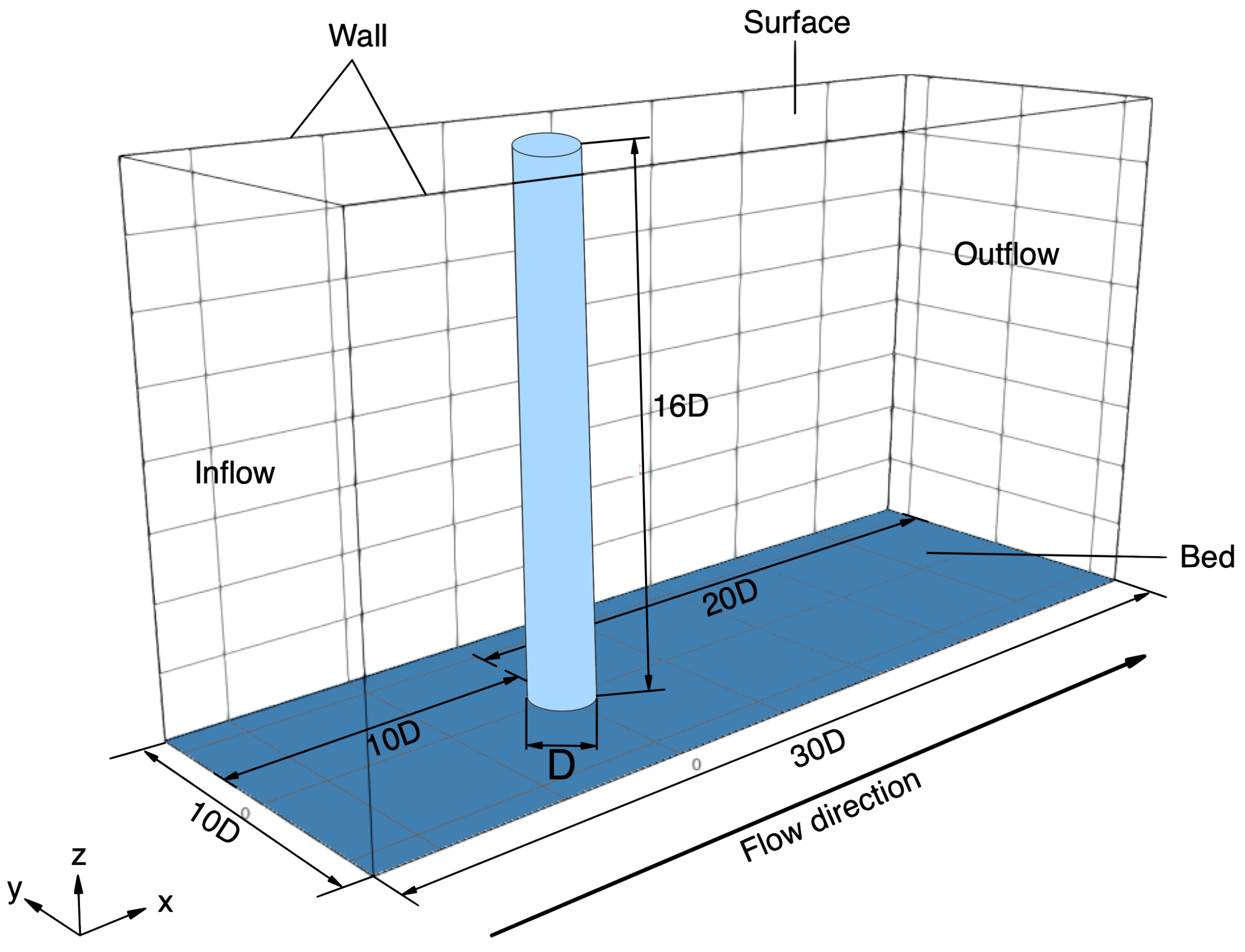
3.1. Configurations of the Computational Domain

As a result of the implementation of the $\sigma$-transformation, the research code can only model partially submerged prismatic obstacles. However, as stated in Lachaussée, 2018 [18], the influence of the height of the obstacle over the scouring process is negligible for $H/D$ larger than 3 (H being the height of the pier), which is the case studied herein. Therefore, a test of height $H=0.09$ m is equivalent to one with $H=0.16$ m due to its diameter being $D=0.01$ m.

Figure 1 shows a global view of the computational domain for the narrow channel case in the present study. The configuration and dimensions are the same as those used in the laboratory experiments performed by Lachaussée, 2018 [18]. The numerical domain is a $30D$ long, $10D$ wide, and $16D$ deep cuboid with a cylinder situated at the axes’ origin, such that the domain is symmetrical in the y-direction with $10D$ upstream and $20D$ downstream of the cylinder.

Figure 2 shows a two-dimensional view of the mesh used in the simulations. The mesh consists of layers of stacked prismatic elements, which are extended from an unstructured triangular 2D mesh in the horizontal direction. To obtain the turbulent flow around the cylinder, the minimum size of the mesh (triangle length l) is set about $l=0.015D$ and $l=0.02D$ in the horizontal and vertical directions, respectively. The largest triangles are close to the walls with an average length of $l=0.25D$ (zone 1). In the middle region (zone 2), the mesh reaches a maximum of $l=0.1D$. Note that higher mesh density is used close to the cylinder (zone 3) to capture the vortex structure. The total number of vertex and cell-centered points in the horizontal are 20,123 and 39,721, respectively. For this mesh, we have 205 vertex points around the cylinder. In the vertical direction, the mesh is comprises 96 layers of elements and the height of the cells increases geometrically as they are further from the bed. The first cell center near the bed is set to be situated in the viscous sub-layer ($z_{+}<5$). In the clear-water case, the first cell center close to the bed is at $z_{+}=2.82$, $u_{+}=23.68$ at the cell center closest to the surface.

3.2. Initial and Boundary Conditions

To validate the numerical model in the clear-water case, we set the problem using the PIV measurements by Lachaussée, 2018 [18]. These measurements were performed close to the bed with a vertical resolution of $\Delta z_{PIV}=8\times {10}^{-4} \mathrm{m}$. To avoid the influence of waves on the scouring process, a plexiglass sheet is put over the water surface to prevent a free surface. Due to the flow conditions, the Froude number $Fr=U/{\left(gh\right)}^2$ is small, so implementing a rigid roof as a surface boundary condition is appropriate. The experimental configuration produces a flow with a mean velocity $U\approx 0.16$ m/s and friction velocity $u_{\tau }\approx 8\pm 1$ mm/s. As ${\mathrm{Re}}_{\tau }\approx 5.4$ in this case, according to Soulsby’s formulation (Equation (13)), the flow approaching the obstacle is in the transitional regime, but very close to being hydraulically smooth. Naturally, as the flow approaches the obstacle and its friction velocity increases, the flow regime is consolidated as transitional.

For the clear-water simulations, we adjust the Swamee profile (14) to the PIV data while confirming that the friction velocity is conserved, and then we apply the profile to the inflow boundary condition. As a result, considering $D=0.01$ m, the pier Reynolds number in the numerical model is ${\mathrm{Re}}_D\approx 2000$.

For the live-bed simulations, the Swamee profile (14) is adjusted to the flow velocity and pier size described in Roulund et al., 2005 [4]. The mean velocity in this case is $U=0.46$ m/s, the pier diameter is $D=0.1$ m, and, therefore, the pier Reynolds number is ${\mathrm{Re}}_D=$ 46,000.

In the present study, the same parameters are used in all the simulations for sediment density, fluid sediment, grain size, sand roughness, bed porosity, critical Shields number for a horizontal slope, and static and dynamic friction coefficients. The parameters used in the tests are summarized in

Table 2. Flow and sediment parameters used for all simulations.

Parameter	Symbol	Clear-Water Case	Live-Bed Case
Mean velocity	U	19.23 cm/s	46 cm/s
Reynolds number	${\mathrm{Re}}_D$	1923	46,000
Friction velocity	$u_{\tau }$	$0.9$ cm/s	$1.8$ cm/s
Water depth	H	16 cm	40 cm
Cylinder diameter	D	1 cm	10 cm
Sediment density	${\rho }_s$	2500 kg m${}^{-3}$	2500 kg m${}^{-3}$
Fluid density	$\rho$	1000 kg m${}^{-3}$	1000 kg m${}^{-3}$
Grain size	d	$0.27$ mm	$0.27$ mm
Sand roughness	$k_s$	$0.67\times {10}^{-3}$ m	$0.67\times {10}^{-3}$ m
Friction Reynolds number	${\mathrm{Re}}_{\tau }$	6	12
Bed porosity	$\eta$	0.4	0.4
Critical Shields number	${\theta }_{c_0}$	0.04	0.04
Dynamic friction coefficient	${\mu }_d$	0.62	0.62
Static friction coefficient	${\mu }_s$	0.63	0.63

.

From the value of ${\theta }_{c_0}$, it follows that the critical friction velocity for the incipient motion of a solid particle on a flat bed is given by Equation (16).

$$u_{\tau crit}={\left[{\theta }_{c_0}gd\left({\rho }_s/\rho -1\right)\right]}^{1/2}=1.27\times {10}^{-2} \mathrm{m}/\mathrm{s}.$$

(16)

Therefore, the ratio $u_{\tau }/u_{\tau crit}$ is equal to 0.72, i.e., clear-water conditions.

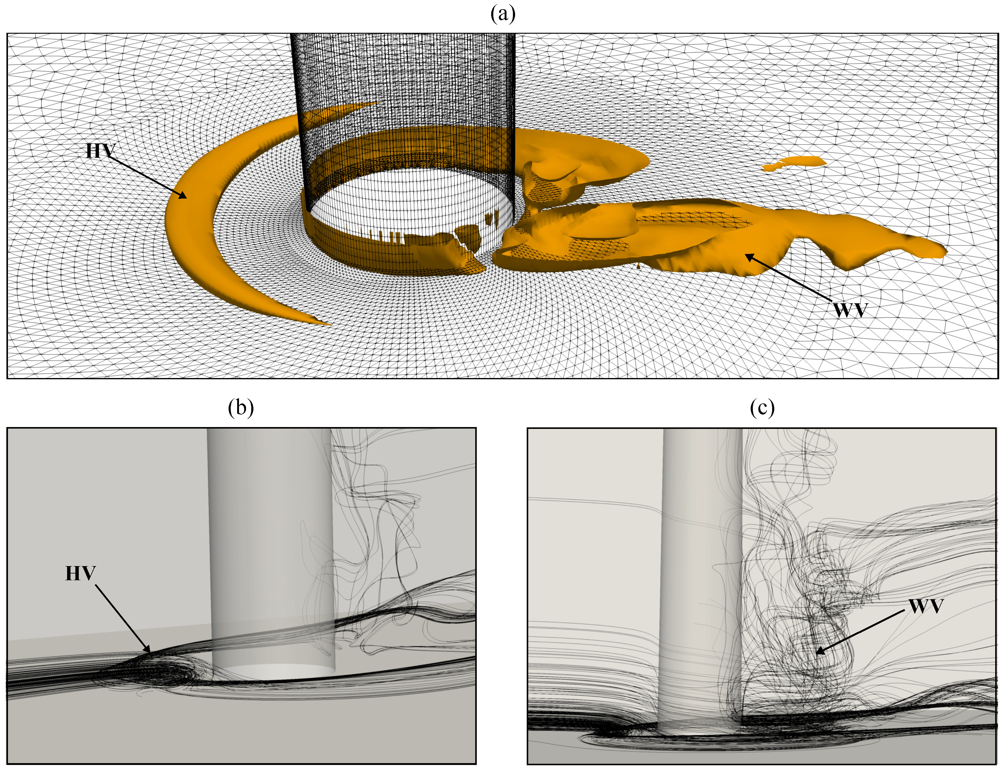
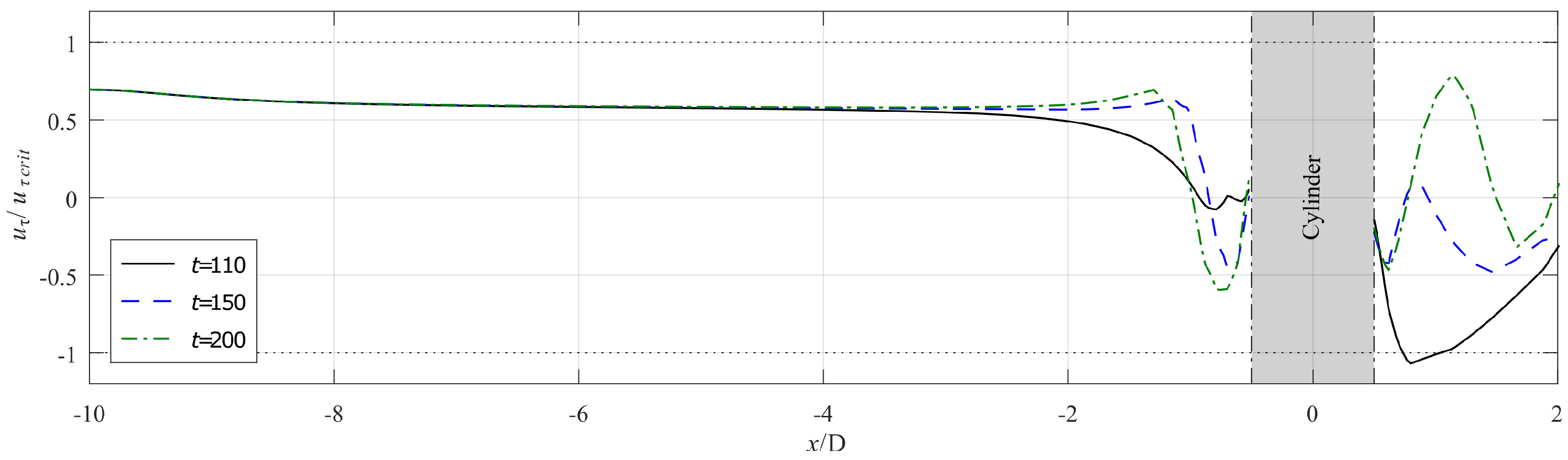
4. Numerical Results

4.1. Live-Bed and Wide Channel Case

As stated in Section 2, the in-house model was validated in Zhang et al., 2020 [20] by reproducing the experimental results in Roulund et al., 2005 [4]. The flow and scour conditions are detailed in the live-bed case in Table 2. In the present study, the Swamee profile defined in Equation (14) is implemented, which differs from the Poiseuille profile utilized in Zhang et al., 2020 [20]. Additionally, the blockage ratio for the wide channel in the present study is $D/W=1/16$, while the blockage ratio in Zhang et al., 2020 [20] is $D/W=1/30$. However, for slip walls, it is considered that the sensitivity of the flow near the obstacle to $D/W$ is minimal when $D/W<0.1$ (Chen et al., 1995 [32] and Lachaussée, 2018 [18]). Therefore, the difference in width can be considered negligible.

Figure 3 compares the experimental measurements from Roulund et al., 2005 [4] corresponding to the rough bed case with a cylinder Reynolds number ${\mathrm{Re}}_D=$ 46,000 with the numerical results of Roulund et al., 2005 [4], and the present study. These results show that the scour depth development over time can still be reproduced after the implementation of the current inflow profile. Furthermore, the current estimation is closer to the experimental data presented originally in Roulund et al., 2005 [4] in terms of scour depth evolution over time.

4.2. Clear-Water Case

This section shows the capability of the proposed numerical model for reproducing the hydrodynamics and morphodynamics behavior around the cylinder in clear-water. The flow results are presented in Figure 4, Figure 5, Figure 6 and Figure 7, and detailed in the section “Hydrodynamic validation”, and the morphological results are presented in Figure 8, Figure 9, Figure 10, Figure 11, Figure 12, Figure 13 and Figure 14, and detailed in the subsection “Morphodynamic validation”. The numerical simulations are performed in two stages to avoid inaccuracies produced by the initial state of the flow. We only compute the hydrodynamic model in the first stage until the flow stabilizes. In the second stage, we calculate both the flow and sediment evolution. In the beginning, the initial condition of the pressure is zero, and the inflow Swamee boundary condition is imposed throughout the domain.

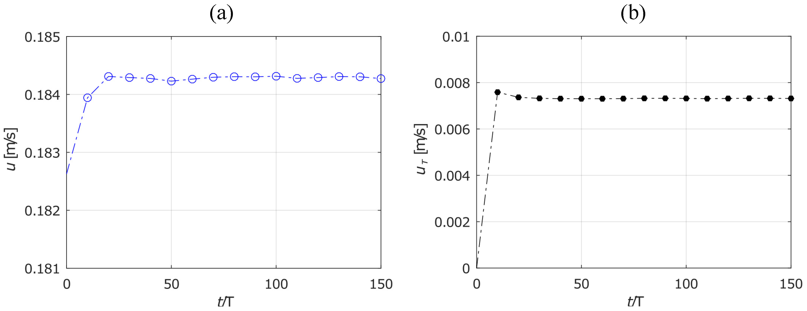
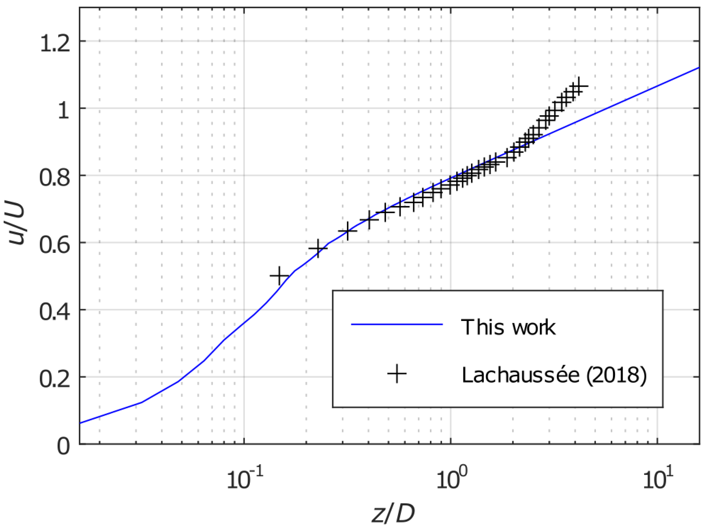
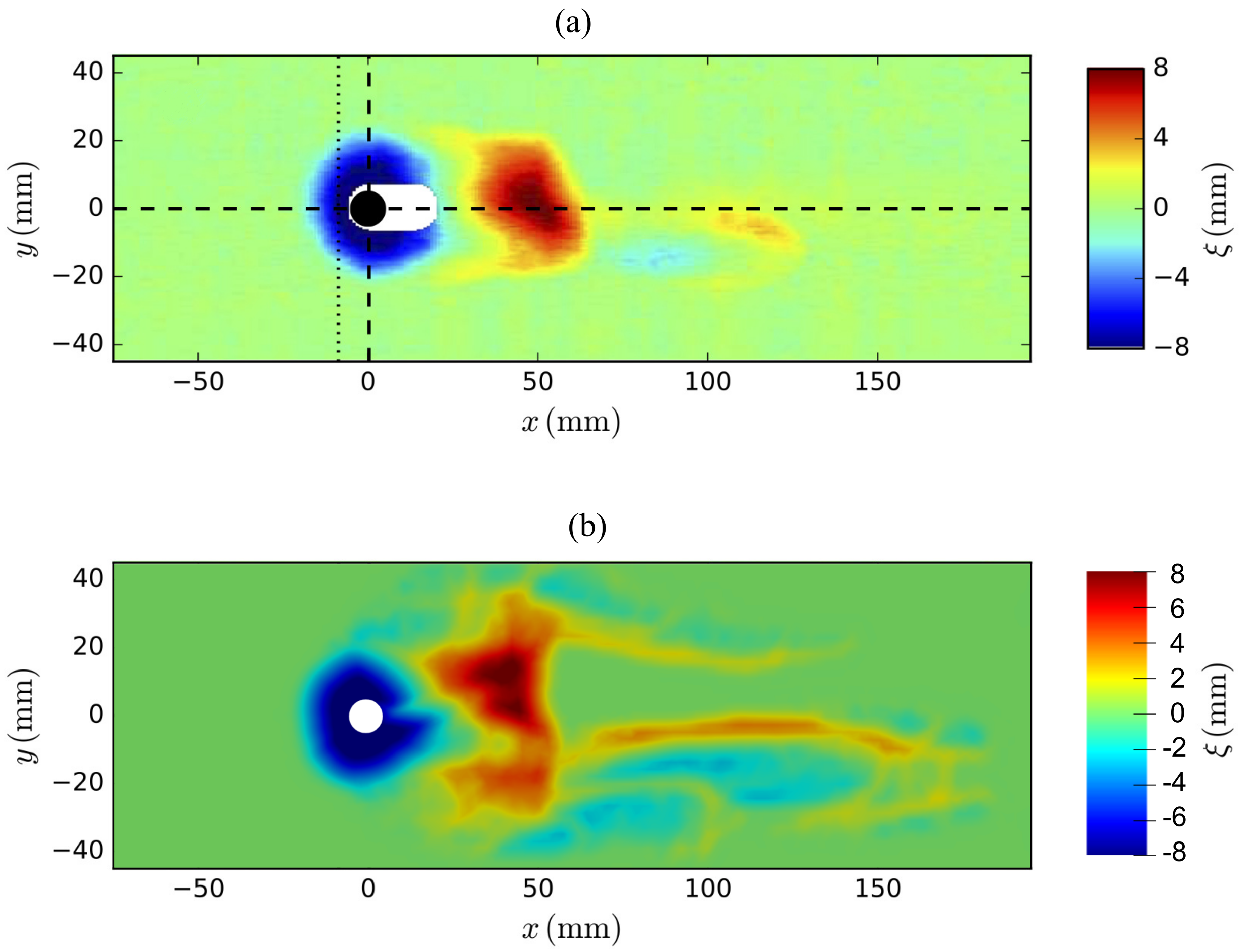
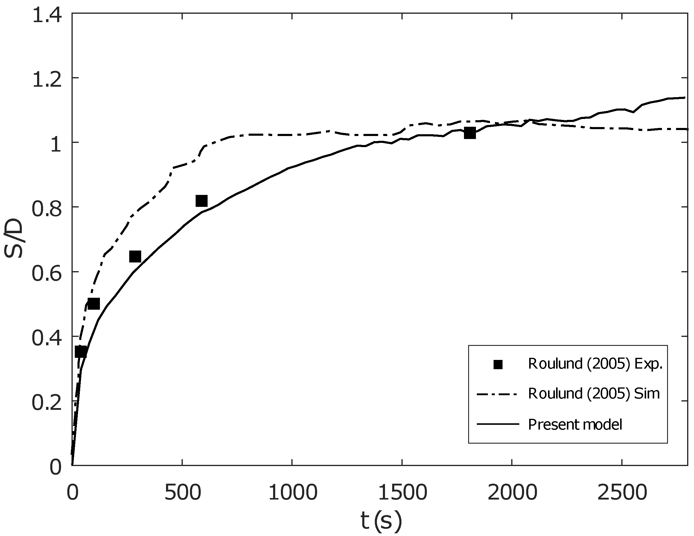
4.2.1. Hydrodynamic Validation

In order to examine the inflow field, the vertical velocity component and the friction velocity are discussed and compared with experimental data in this section. The evolution of the flow is analyzed to find the time needed for the velocity to reach an equilibrium. The study of morphological evolution begins at the conclusion of this warm-up time.

Figure 4 presents the time evolution of the velocity at the first vertical cell and the friction velocity results. Note that both quantities stabilize as expected. Moreover, there are no significant changes after $t/T=60$. This time agrees with the non-dimensional time necessary for the flow to travel twice the distance from the inlet to the outlet. It is also equivalent to dimensional 3.12 s using a time scale of $T=0.052$ s. Figure 5 compares the vertical profile of the resolved approaching flow at $x/D=-5$ and $t/T=100$ with the experimental measurements in Lachaussée, 2018 [18]. This velocity profile is close to the PIV measurements for $z/D<2$, which is the critical region for scour erosion. In the present study, the warm-up time is set to $t/T=100$.

Figure 4. Time analysis of (a) the velocity at the first vertical cell above the bed, and (b) the friction velocity for a flow with ${\mathrm{Re}}_D\approx 2000$ at $(x,y)=(-5,0)$.

Figure 4. Time analysis of (a) the velocity at the first vertical cell above the bed, and (b) the friction velocity for a flow with ${\mathrm{Re}}_D\approx 2000$ at $(x,y)=(-5,0)$.

Figure 5. Comparison between the numerical vertical velocity profile at $(x,y)=(-5,0)$ and the PIV measurements in Lachaussée, 2018 [18] for the flow with ${\mathrm{Re}}_D\approx 2000$ and $U=0.1923$ m/s.

Figure 5. Comparison between the numerical vertical velocity profile at $(x,y)=(-5,0)$ and the PIV measurements in Lachaussée, 2018 [18] for the flow with ${\mathrm{Re}}_D\approx 2000$ and $U=0.1923$ m/s.

Figure 6 displays the three-dimensional instantaneous flow at the non-dimensional time $t/T=100$, just before the beginning of the second stage. The cylinder is represented by the gray surface and the flow by the black streamlines. Note the complex patterns of the streamlines close to the cylinder. The adverse pressure gradients induced by the cylinder obstruction create downflows in front of the cylinder and generate a horseshoe vortex (HV) near the bottom and wake region behind the cylinder. Figure 6a shows the main coherent structure in an instantaneous flow associated with an HV using the Q criterion. We clearly observed a clockwise vortex close to the bottom in Figure 6b, which also presents 3D streamlines of the wake region behind the cylinder. Figure 6c presents 3D streamlines of the wake region behind the cylinder. We note fluid particles situated close to the bed could be first entrained into the core of this region, and then, from there, toward the surface by an upwelling anti-clockwise vortex. This counter-clockwise rotating vortex would be responsible for the scour mechanisms downstream of the cylinder.

Figure 6. Three-dimensional instantaneous flow visualization at $t/T=100$: (a) Detailed view of the vortex structures at the base of the cylinder. (b) Front and (c) side view depicting stream lines.

Figure 6. Three-dimensional instantaneous flow visualization at $t/T=100$: (a) Detailed view of the vortex structures at the base of the cylinder. (b) Front and (c) side view depicting stream lines.

Finally, Figure 7 shows the horizontal profile of the friction velocity amplification over the line $y=0$ at different time stages. Here, $u_{\tau crit}=1.27\times {10}^{-2} \mathrm{m}/\mathrm{s}$ as defined in Equation (16). In this case, the sediment transport starts at $t/T=100$. Before a dune is formed, the friction velocity slightly surpasses the critical value. It is worth noting that the distance between the inflow boundary and the cylinder is enough to stabilize the flow. Thus, the friction velocity reaches an equilibrium value of $8\pm 1$ mm/s, remaining unperturbed as long as it is far enough from the cylinder. This value agrees with the measurements given by Lachaussée, 2018 [18].

Figure 7. Friction velocity amplification along the x direction with $y=0$ for ${\mathrm{Re}}_D\approx 2000$.

Figure 7. Friction velocity amplification along the x direction with $y=0$ for ${\mathrm{Re}}_D\approx 2000$.

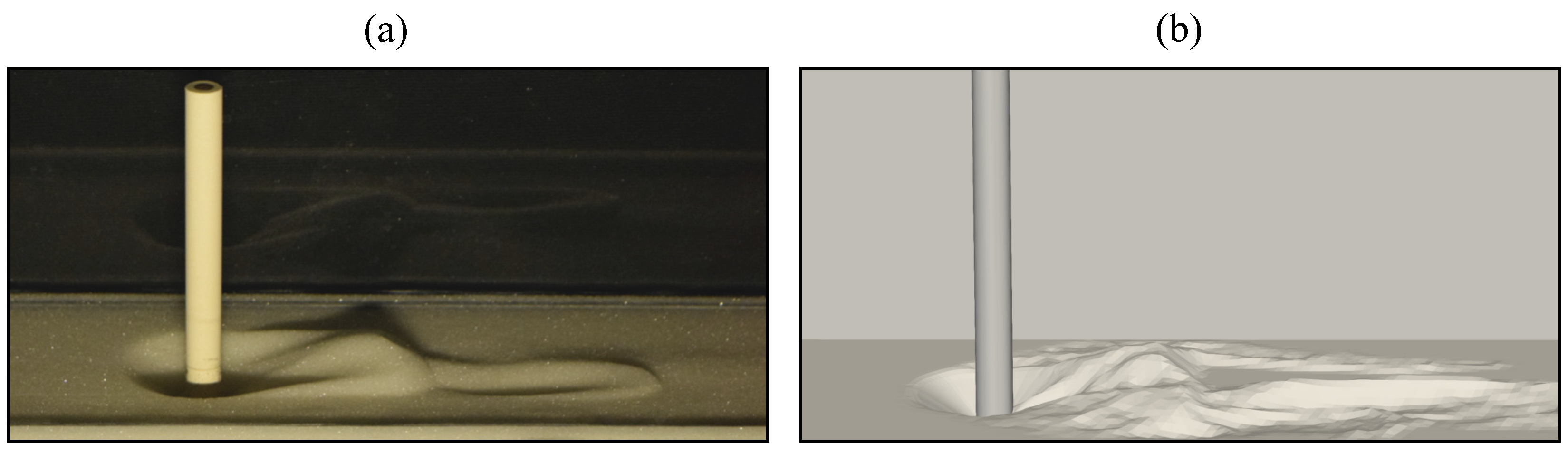
4.2.2. Morphodynamic Validation

This section is devoted to the analysis of the scour around the cylinder. The morphological model is tested for ${\mathrm{Re}}_D\approx 2000$, in the clear-water regime. Any friction velocity greater than $1.27\times {10}^{-2}$ m/s will result in a Shields number satisfying the condition $\theta >{\theta }_{c0}$, and, thus, it will produce sediment transport. Figure 8 illustrates the early evolution of the obtained scour hole at non-dimensional morphological times t/$T\ast$ equal to 100, 200, 400, and 800. At these early stages, the development of the scour hole agrees qualitatively with the one presented for live-bed conditions in Zhang et al., 2021 [19]. $T\ast$ is the morphological time scale defined by Sumer, 1992 [46] as follows:

$$T\ast =\frac{D^2}{\sqrt{g(s-1)d^3}},$$

(17)

where d is the grain size and $s={\rho }_s/\rho$ is the relative density of the sediment. In this case, $T\ast =5.87$.

Figure 8. Bed elevation near the cylinder at different moments in time, demonstrating the evolution of the scour hole.

Figure 8. Bed elevation near the cylinder at different moments in time, demonstrating the evolution of the scour hole.

Figure 9 presents the horizontal profiles of the same results shown in Figure 8, offering a more quantitative insight into the scour hole and the dune. The scour hole upstream of the cylinder presents a consistent angle of approximately 32°, which is consistent with the prescribed value for the maximum angle of repose in Lachaussée et al., 2018 [16]. By contrast, the dune downstream of the cylinder does not have a consistent shape throughout its formation. While the lee-side angle of the dune is unchanged once it reaches the same slope as the scour hole, the stoss side of the dune presents more inconsistency. This last behavior might result from the wake vortices interacting directly on the stoss side of the dune.

Figure 9. Horizontal profile of the bed elevation at $y=0$, corresponding to the same states shown in Figure 8.

Figure 9. Horizontal profile of the bed elevation at $y=0$, corresponding to the same states shown in Figure 8.

Additionally, the presence of a horseshoe vortex in the studied range of ${\mathrm{Re}}_D$ is in agreement with Baker, 1979 [47]. The presence of scour induced by the horseshoe vortex (herein referred to as “horseshoe scour”) in clear-water regime agrees with Lachaussée et al., 2018 [16]. Three measures are compared with their data: the maximum depth ${\xi }_m$ and the characteristic lengths $L_x$ and $L_y$, illustrated in Figure 10. $L_x$ is defined as the distance between the pier and the point of the bed where its depth is ${\xi }_m/2$. $L_y$ is also defined as the distance between the pier and the point of the bed where its depth is ${\xi }_m/2$.

Figure 10. Characteristic lengths of the scour hole.

Figure 10. Characteristic lengths of the scour hole.

The time evolution of ${\xi }_m$, $L_x$, and $L_y$ can be fit to the exponential law

$$f\left(t\right)=A\left(1-Bexp\left(-\frac{t}{T_a}\right)-(1-B)exp\left(-\frac{t}{10T_a}\right)\right),$$

(18)

where A, B, and $T_a$ are empirical parameters. This is illustrated in Figure 11a, where the square, triangle, and circle markers are the computed maximum depth, and the upstream and lateral characteristic lengths, respectively. The solid and dashed lines are the adjusted Equation (18) to fit the evolution of ${\xi }_m$, $L_x$, and $L_y$.

Figure 11 presents a comparison between the numerical and experimental results with the model Equation (18). Figure 11a illustrates the fitting of the Equation (18) to the numerical data. The values for the empirical parameters are $A=-10.3$, $B=0.6$, and $T_a=1000$ for the time evolution of ${\xi }_m$; $A=14.5$, $B=0.42$, and $T_a=1000$ for the time evolution of $L_x$, and $A=15$, $B=0.52$, and $T_a=1000$ for the time evolution of $L_y$.

Figure 11. (a) Time evolution of ${\xi }_m$, $L_x$, and $L_y$. (b) Comparison between the numerical and experimental data.

Figure 11. (a) Time evolution of ${\xi }_m$, $L_x$, and $L_y$. (b) Comparison between the numerical and experimental data.

As illustrated by Figure 11b, initially, the scour evolution in the numerical results fits well with the experimental results of Lachaussée, 2018 [18], but the model eventually over-predicts the maximum scour depth. With regard to the characteristic lengths, the numerical results present a better fit for $L_y$ than $L_x$. This is because the numerical results present a rounder scour hole than the one in the experiment. As a comment, we note that the maximum depth of the predicted scour hole is often situated in a region that, in the experimental case, was obscured by the pier, and thus could not be measured.

Figure 12 shows a comparison between the numerical results of the present study and the experimental results with equivalent flow and sediment conditions reported in the thesis of Lachaussée, 2018 [18]. Both the scour hole and the dune have a similar magnitude and angle, with some discrepancy around the limits of the scour hole and downstream of the dune. The numerical and experimental data in the figure both correspond to an instant in which the scour hole has not yet reached an equilibrium.

Figure 12. Comparison between the numerical results at a non-dimensional time $t/T=3500$ and the experimental results reported in Lachaussée, 2018 [18] at time $t=2.4$ h. The horizontal profiles were extracted along the lines $y=0$ (a), $x=0$ (b), and $x=-9$ mm (c).

Figure 12. Comparison between the numerical results at a non-dimensional time $t/T=3500$ and the experimental results reported in Lachaussée, 2018 [18] at time $t=2.4$ h. The horizontal profiles were extracted along the lines $y=0$ (a), $x=0$ (b), and $x=-9$ mm (c).

Figure 13 shows a topographical comparison at the same time as Figure 12. The shape and magnitude of the predicted scour hole is very similar to that of the experimental results. However, while the position and magnitude of the dune in the numerical results agree with the experimental ones, the width is different. A shallow scour hole is present at the lee-side of the dune, which is in agreement with the experimental results, although the one predicted is larger.

This second scour hole seems to be a result of the non-slip conditions at the lateral walls, as these conditions model the physical walls of a narrow channel. This scour hole is an example of wake scour, as the wake of the cylinder is trapped inside the channel, producing scour at the lee-side of the dune. A 3D view is shown in Figure 14.

Figure 13. (a) Topographical map of the experimental results reported in Lachaussée, 2018 [18] at time $t=2.4$ h. (b) Topographical map of the state of the sediment bed for the numerical results at non-dimensional time $t/T=3500$.

Figure 13. (a) Topographical map of the experimental results reported in Lachaussée, 2018 [18] at time $t=2.4$ h. (b) Topographical map of the state of the sediment bed for the numerical results at non-dimensional time $t/T=3500$.

Figure 14. (a) Snapshot of the scour in development at time $t=2.4$ h (Lachaussée, 2018 [18]). (b) Scour hole at non-dimensional time $t/T=3500$.

Figure 14. (a) Snapshot of the scour in development at time $t=2.4$ h (Lachaussée, 2018 [18]). (b) Scour hole at non-dimensional time $t/T=3500$.

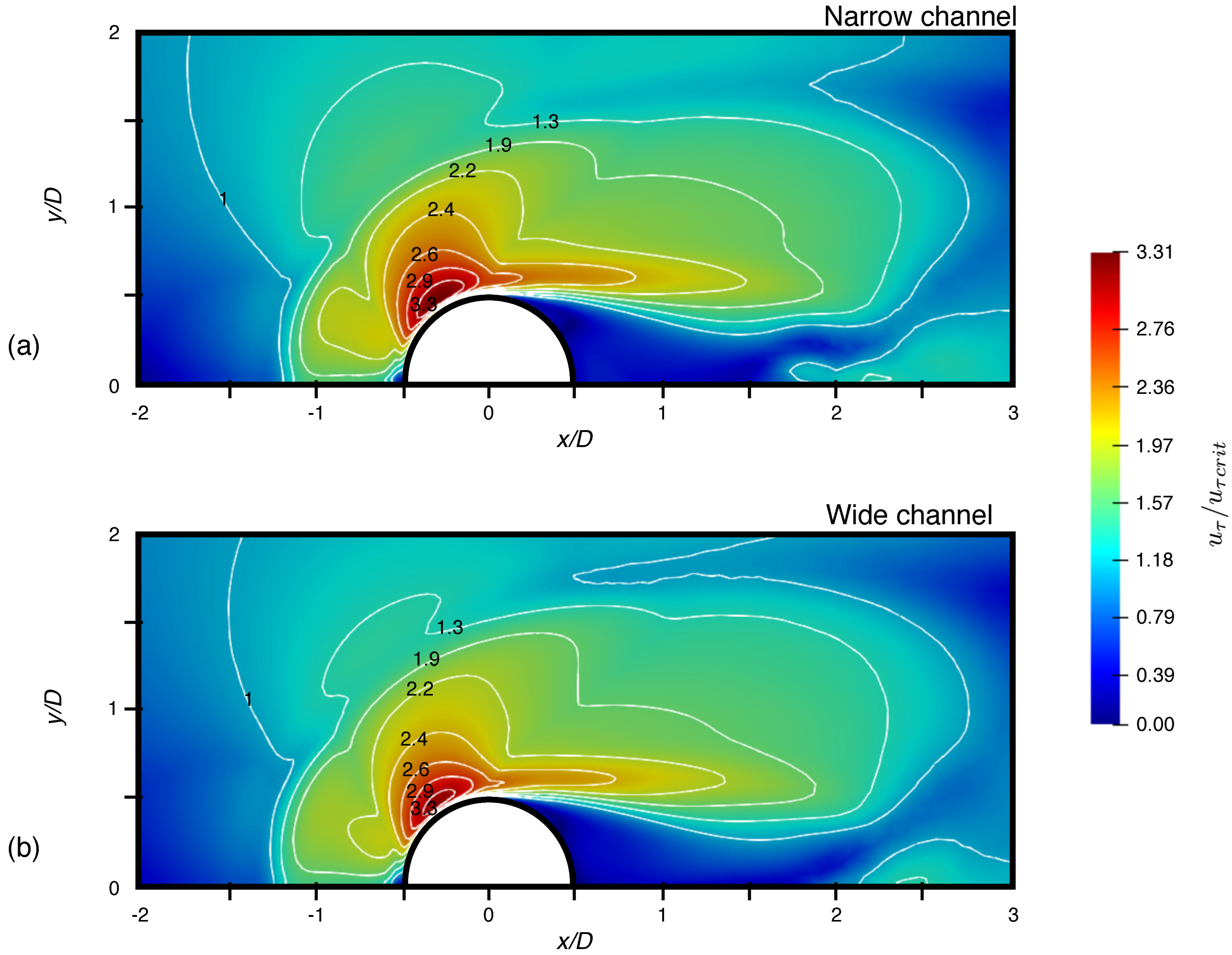
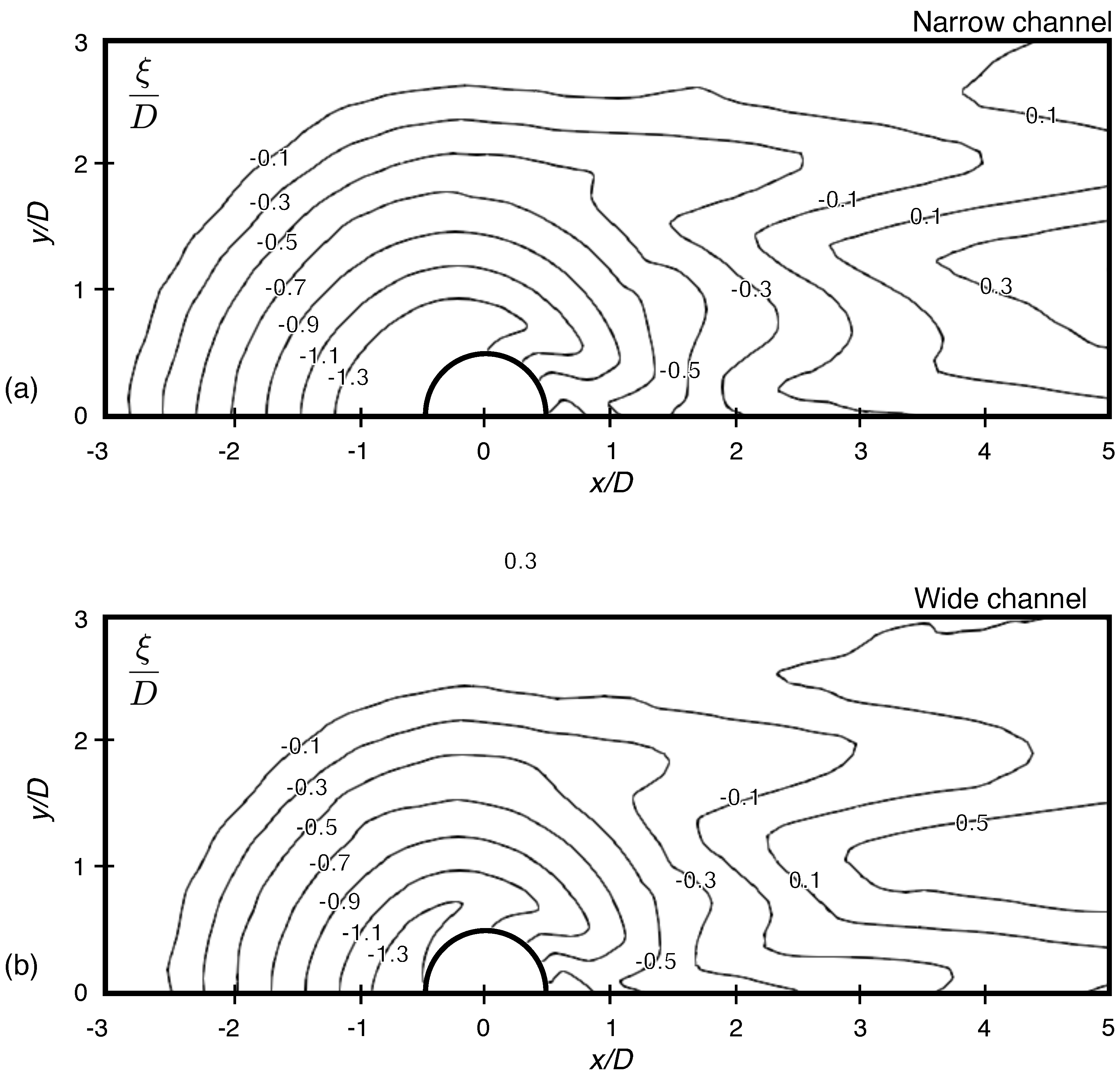
4.3. Effects of the Channel Width on the Clear-Water Local Scour Pattern

In a free-stream, the streamlines lateral to an obstacle will contract, resulting in flow acceleration. If the flow acceleration results in a supercritical Shields number, the sediment particles will be set in motion, resulting in scouring. In a narrow channel, the flow is confined between two lateral walls, and this confinement will accentuate the contraction of the streamlines, further accelerating the flow past the obstacle. Under this contraction effect, the dune will be pushed downstream. In clear-water conditions, the region of threshold overshoot has a larger expansion than in live-bed conditions. In this section, the narrow channel case has a blockage ratio of $D/W=0.1$, and the wide channel has a blockage ratio $D/W=0.0625$.

Figure 15 shows the friction velocity amplification $u_{\tau }/u_{\tau crit}$, where $u_{\tau crit}$ is as defined in Equation (16). The figures show the amplification effect of the friction velocity at the sides of the cylinder. Roulund et al., 2005 [4], describes this amplification as being caused by the contraction of the flow streamlines and the horseshoe vortex. The isolines in Figure 15a show that the largest amplification is located at an angle within the interval ${43}^{\circ }\le \phi \le {75}^{\circ }$. This region is approximately 45 percent wider than the equivalent region in the wide channel case, which is located at ${48}^{\circ }\le \phi \le {70}^{\circ }$ (Figure 15b). In the narrow channel case, the confinement of the flow results in a larger contracted area relative to the wide channel case, which will result in a larger sediment transport rate at the start of the development.

Figure 16 compares the resulting bed topography of the clear-water simulations. It can be seen that both scour holes and dunes present similar characteristics. The horseshoe scour hole is circular without reaching the wake-side of the cylinder. The maximum scour depth is present in both cases at the lee-side of the cylinder, lateral to the stagnation point, at $|y/D|\approx 0.25D$. The scour hole in the narrow channel is deeper than the scour hole in the wide channel by approximately $15\%$.

Figure 17 compares the time evolution of the normalized scour depth for the three scour simulations performed for the present study. Regarding clear-water, it can be observed that, in both cases, the scour depth evolution is largely monotonically increasing. This continuously growing scour behaviour, although not perfectly monotonic in lab studies, has been documented in experimental studies on clear-water scour, such as Lachaussée, 2018 [18], Kothyari et al., 2007 [48], and Melville et al., 1999 [2]. Moreover, the scour rate decreases over time in both cases. From the the beginning of the scour simulation, both cases presented a similar scour evolution, but the scour rate decreases more rapidly for the wide channel case. This initial similar behavior can be explained by the similar magnitude reached by the friction velocity in the rigid bed simulation (Figure 16). The area where the friction velocity overshoots its critical value is only slightly larger in the narrow channel case, so the faster scour rate does not become apparent in the early time of the simulation. As a result, the narrow channel effect results in a faster scour process and a deeper horseshoe scour hole in the clear-water test, as shown in Figure 16.

It is important to note that the live-bed tests were based on the configuration in Roulund et al., 2005 [4], while the clear-water conditions are based on the configuration in Lachaussée, 2018 [18]. A notable difference is the pier diameter, which affects the relative coarseness (D/d) of the model. In the Roulund configuration, $D/d\approx 370$, while in the Lachaussée case $D/d\approx 37$. Several studies have pointed out the influence of the relative coarseness on the effect of the blockage ratio over the scouring process. Tejada, 2014 [49], states that, for $D/d<100$, the blockage ratio has minimal influence over the scour process. However, an experimental study by Williams et al., 2018 [6], was performed with a relative coarseness $D/d=81$ and it was found that the larger blockage ratio produced a larger scour depth. This suggests that the relationship between the relative coarseness and the blockage ratio may be more complex than previously thought.

The effect of the roughness length $z_0$ over the scouring process is a similar consideration to the relative coarseness effect. The behavior of $z_0$, which directly influences the friction velocity, is directly influenced by the hydraulic regime of the flow (Equation (13)). It can be seen in Table 2 that the clear-water case is located in the transitional hydraulic regime, but very close to the smooth hydraulic regime at ${\mathrm{Re}}_D\approx 6$. Furthermore, considering the largest amplification factor seen in Figure 15, we obtain ${\mathrm{Re}}_D\approx 22.8$, which is within the transitional hydraulic regime. In contrast, the live-bed configuration (Table 2) results in a larger friction velocity amplification near the cylinder (Zhang et al., 2020 [20]), which locally overshoots the threshold for the rough hydraulic regime.

5. Conclusions

Despite important research efforts over the last decade, there are still difficulties in accurately predict the maximum value of $S/D$ (Harasti et al., 2023 [50]). It is for this reason that a correct understanding of the kinematics of the scour at the base of an obstacle are vital for designing and constructing sustainable hydraulic structures. This study presents a numerical model using the LES approach. The code was initially developed by Zhang et al., 2020 [20] for a wide channel in live-bed conditions in the turbulent rough regime (${\mathrm{Re}}_D\approx$ 46,000). In the present study, we successfully studied the combined effect of the velocity and the blockage with a focus on an approaching flow near the hydraulically smooth regime. We consider two different test cases. The first case presents a good agreement with the experimental findings of Roulund et al., 2005 [4] (${\mathrm{Re}}_D\approx$ 46,000), with the objective of acting as a control case to ensure that the model could still accurately predict the scouring process in the live-bed regime after the extension of the applicability to the clear-water regime and the generalization of the flow conditions. A moderately low Reynolds number (${\mathrm{Re}}_D\approx 2000$) is used for the second case to study the model’s ability to predict clear-water scour. Validation is achieved by qualitatively and quantitatively comparing the predicted scour depth and time evolution with a laboratory experiment reported in Lachaussée, 2018 [18].

We obtain fair agreement with the velocity profile obtained using PIV measurements in the narrow channel with non-slip lateral wall boundary conditions. Although the numerical model still has discrepancies at the lee-side of the dune and downstream of it, the accuracy of the predicted angle, size, and depth of the scour hole are very good near the obstacle. This is despite the difference in the height of the cylinder and despite the fact that the experimental set-up uses a submerged cylinder while the cylinder in the numerical set-up is only partially submerged. This behavior is consistent with the conclusion regarding the height–diameter ratio of the obstacle in Lachaussée, 2018 [18]. The model can also accurately predict the depth evolution of the scour hole. However, in the long-term simulation, the model reaches its equilibrium at a greater depth. This behavior could be a consequence of the sediment bed hypothesis as a continuum, the pier “shadow effect” on the measurement technique, or a combination of both.

The amplification to the flow contraction caused by the confinement is well described by the model. In the clear-water case, the narrow channel simulation presented a higher scour depth than the wide channel simulation. These results show that a large blockage ratio ($D/W\ge 0.1$) can have an important impact over the scour process, despite a low relative coarseness ($D/d<100$). However, because all tests in the present study were performed for low Froude number values, it would be interesting to perform a similar study for a higher value Froude number to account for the free surface effects on the scouring process. Future study will focus on testing similar flow conditions with different pier geometries.

References

1. Raudkivi, A.; Ettema, R. Clear-water scour at cylindrical piers. J. Hydraul. Eng. 1983, 109, 338–350. [Google Scholar] [CrossRef]
2. Melville, B.W.; Chiew, Y.M. Time scale for local scour at bridge piers. J. Hydraul. Eng. 1999, 125, 59–65. [Google Scholar] [CrossRef]
3. Ettema, R.; Constantinescu, G.; Melville, B.W. Flow-field complexity and design estimation of pier-scour depth: Sixty years since Laursen and Toch. J. Hydraul. Eng. 2017, 143, 03117006. [Google Scholar] [CrossRef]
4. Roulund, A.; Sumer, B.M.; Fredsøe, J.; Michelsen, J. Numerical and experimental investigation of flow and scour around a circular pile. J. Fluid Mech. 2005, 534, 351–401. [Google Scholar] [CrossRef]
5. Stevens, M.A.; Gasser, M.M.; Saad, M.B.A.M. Wake Vortex Scour at Bridge Piers. J. Hydraul. Eng. 1991, 117, 891–904. [Google Scholar] [CrossRef]
6. Williams, P.; Bolisetti, T.; Balachandar, R. Blockage correction for pier scour experiments. Can. J. Civ. Eng. 2018, 45, 413–417. [Google Scholar] [CrossRef]
7. Proske, D. Bridge Collapse Frequencies versus Failure Probabilities; Springer: Berlin, Germany, 2018. [Google Scholar]
8. Arneson, L.; Zevenbergen, L.; Lagasse, P.; Clopper, P. Evaluating Scour at Bridges; Technical Report; Federal Highway Administration: Fort Collins, CO, USA, 2012.
9. Huber, F. Update: Bridge scour. ASCE 1991, 61, 62–63. [Google Scholar]
10. Wardhana, K.; Hadipriono, F.C. Analysis of recent bridge failures in the United States. J. Perform. Constr. Facil. 2003, 17, 144–150. [Google Scholar] [CrossRef]
11. Lin, C.; Han, J.; Bennett, C.; Parsons, R.L. Case history analysis of bridge failures due to scour. In Climatic Effects on Pavement and Geotechnical Infrastructure; American Society of Civil Engineers: Reston, VA, USA, 2014; pp. 204–216. [Google Scholar] [CrossRef]
12. Taricska, M. An Analysis of Recent Bridge Failures (2000–2012). Master’s Thesis, Ohio State University, Columbus, OH, USA, 2014. [Google Scholar]
13. Kirkil, G.; Constantinescu, G. Nature of flow and turbulence structure around an in-stream vertical plate in a shallow channel and the implications for sediment erosion. Water Resour. Res. 2009, 45, W06412. [Google Scholar] [CrossRef]
14. Kirkil, G.; Constantinescu, G. A numerical study of the laminar necklace vortex system and its effect on the wake for a circular cylinder. Phys. Fluids 2012, 24, 073602. [Google Scholar] [CrossRef]
15. Kirkil, G.; Constantinescu, G. Effects of cylinder Reynolds number on the turbulent horseshoe vortex system and near wake of a surface-mounted circular cylinder. Phys. Fluids 2015, 27, 075102. [Google Scholar] [CrossRef]
16. Lachaussée, F.; Bertho, Y.; Morize, C.; Sauret, A.; Gondret, P. Competitive dynamics of two erosion patterns around a cylinder. Phys. Rev. Fluids 2018, 3, 012302. [Google Scholar] [CrossRef]
17. Lai, Y.G.; Liu, X.; Bombardelli, F.A.; Song, Y. Three-Dimensional Numerical Modeling of Local Scour: A State-of-the-Art Review and Perspective. J. Hydraul. Eng. 2022, 148, 03122002. [Google Scholar] [CrossRef]
18. Lachaussée, F. Érosion et Transport de Particules au Voisinage d’un Obstacle (in French). Ph.D. Thesis, Université Paris-Saclay, Paris, France, 2018. Available online: https://www.theses.fr/2018SACLS377 (accessed on 24 July 2023).
19. Zhang, W.; Uh Zapata, M.; Pham Van Bang, D.; Nguyen, K.D. Three-Dimensional Hydrostatic Curved Channel Flow Simulations Using Non-Staggered Triangular Grids. Water 2022, 14, 174. [Google Scholar] [CrossRef]
20. Zhang, W.; Uh Zapata, M.; Bai, X.; Pham Van Bang, D.; Nguyen, K.D. Three-dimensional simulation of horseshoe vortex and local scour around a vertical cylinder using an unstructured finite-volume technique. Int. J. Sediment Res. 2020, 35, 295–306. [Google Scholar] [CrossRef]
21. Yu, P.; Zhu, L. Numerical simulation of local scour around bridge piers using novel inlet turbulent boundary conditions. Ocean Eng. 2020, 218, 108166. [Google Scholar] [CrossRef]
22. Jia, Y.; Altinakar, M.; Guney, S. Three-dimensional numerical simulations of local scouring around bridge piers. J. Hydraul. Res. 2017, 56, 351–366. [Google Scholar] [CrossRef]
23. Xiong, W.; Tang, P.; Kong, B. Computational Simulation of Live-Bed Bridge Scour Considering Suspended Sediment Loads. J. Comput. Civ. Eng. 2017, 31, 04017040. [Google Scholar] [CrossRef]
24. Baykal, C.; Sumer, B.M.; Fuhrman, D.R.; Jacobsen, N.G.; Fredsøe, J. Numerical investigation of flow and scour around a vertical circular cylinder. Phil. Trans. R. Soc. A 2015, 373, 104. [Google Scholar] [CrossRef]
25. Baykal, C.; Sumer, B.M.; Fuhrman, D.R.; Jacobsen, N.G.; Fredsøe, J. Numerical simulation of scour and backfilling processes around a circular pile in waves. Coast. Eng. 2017, 122, 87–107. [Google Scholar] [CrossRef]
26. Olsen, N.; Melaaen, C. Three-dimensional calculation of scour around cylinders. J. Hydraul. Mech. 1993, 119, 1048–1054. [Google Scholar] [CrossRef]
27. Zhao, M.; Cheng, L.; Zang, Z. Experimental and numerical investigation of local scour around a submerged vertical circular cylinder in steady currents. Coast. Eng. 2010, 57, 709–721. [Google Scholar] [CrossRef]
28. Khosronejad, A.; Flora, K.; Sotiropoulos, F. Experimental and computational investigation of local scour around bridge piers. Water Resour. 2012, 37, 73–85. [Google Scholar] [CrossRef]
29. Link, O.; González, C.; Maldonado, M.; Escauriaza, C. Coherent structure dynamics and sediment particle motion around a cylindrical pier in developing scour hole. Acta Geophys. 2012, 60, 1689–1719. [Google Scholar] [CrossRef]
30. Van Rijn, L.C. Principles of Sediment Transport in Rivers, Estuaries And Coastal Seas; Aqua Publications: Amsterdam, The Netherlands, 1993. [Google Scholar]
31. Zhang, W. 3D Numerical Simulation of Scour Erosion Around an Obstacle. Ph.D. Thesis, Université Paris-Est, Paris, France, 2019. [Google Scholar]
32. Chen, J.H.; Pritchard, W.G.; Tavener, S.J. Bifurcation for flow past a cylinder between parallel planes. J. Fluid Mech. 1995, 284, 23–41. [Google Scholar] [CrossRef]
33. Singha, S.; Sinhamahapatra, K.P. Flow past a circular cylinder between parallel walls at low Reynolds numbers. Ocean Eng. 2010, 37, 757–769. [Google Scholar] [CrossRef]
34. Mignot, E.; Moyne, T.; Doppler, D.; Riviere, N. Clear-Water Scouring Process in a Flow in Supercritical Regime. J. Hydraul. Eng. 2015, 142, 04015063. [Google Scholar] [CrossRef]
35. Engelund, F.; Fredsøe, J. A sediment transport model for straight alluvial channels. Hydrol. Res. 1976, 7, 293–306. [Google Scholar] [CrossRef]
36. Bento, A.M.; Pêgo, J.P.; Viseu, T.; Couto, L. Scour Development Around an Oblong Bridge Pier: A Numerical and Experimental Study. Water 2023, 15, 2867. [Google Scholar] [CrossRef]
37. Mason, P.J.; Thomson, D.J. Stochastic backscatter in large-eddy simulations of boundary layers. J. Fluid Mech. 1992, 242, 51. [Google Scholar] [CrossRef]
38. Nikuradse, J. Laws of Flow in Rough Pipes; Technical Memorandum 1292; National Advisory Committee for Aeronautics: Washington, DC, USA, 1950.
39. Roulsby, R. Dynamics of Marine Sands: A Manual for Practical Applications; Thomas Telford: London, UK, 1997. [Google Scholar]
40. Swamee, P.K. Generalized inner region velocity distribution equation. J. Hydraul. Eng. 1993, 119, 651–656. [Google Scholar] [CrossRef]
41. Uh Zapata, M.; Pham Van Bang, D.; Nguyen, K.D. An unstructured finite volume technique for the 3D Poisson equation on arbitrary geometry using a sigma-coordinate system. Int. J. Numer. Methods Fluids 2014, 76, 611–631. [Google Scholar] [CrossRef]
42. Uh Zapata, M.; Pham Van Bang, D.; Nguyen, K.D. Unstructured Finite-Volume Model of Sediment Scouring Due to Wave Impact on Vertical Seawalls. J. Mar. Sci. Eng. 2021, 9, 1440. [Google Scholar] [CrossRef]
43. Phillips, N.A. A coordinate system having some special advantages for numerical forecasting. J. Meteor. 1957, 14, 184–185. [Google Scholar] [CrossRef]
44. Chorin, A.J. Numerical solution of the Navier-Stokes equations. Math. Comput. 1968, 22, 745–762. [Google Scholar] [CrossRef]
45. Uh Zapata, M.; Zhang, W.; Pham Van Bang, D.; Nguyen, K.D. A parallel second-order unstructured finite volume method for 3D free-surface flows using a σ coordinate. Comput. Fluids 2019, 190, 15–29. [Google Scholar] [CrossRef]
46. Sumer, B.; Fredsøe, J.; Christiansen, N. Scour around vertical pile in waves. J. Waterw. Port Coast. Ocean Eng. 1992, 118, 15–31. [Google Scholar] [CrossRef]
47. Baker, C.J. The laminar horseshoe vortex. J. Fluid Mech. 1979, 95, 347–367. [Google Scholar] [CrossRef]
48. Kothyari, U.; HAger, W.H.; Oliveto, G. Generalized approach for clear-water scour at bridge foundation elements. J. Hydraul. Eng. 2007, 133, 1229–1240. [Google Scholar] [CrossRef]
49. Tejada, S. Effects of Blockage and Relative Coarseness on Clear Water Bridge Pier Scour. Master’s Thesis, University of Windsor, Windsor, ON, Canada, 2014. Available online: https://scholar.uwindsor.ca/etd/5055/ (accessed on 24 July 2023).
50. Harasti, A.; Gilja, G.; Adžaga, N.; Žic, M. Analysis of Variables Influencing Scour on Large Sand-Bed Rivers Conducted Using Field Data. Appl. Sci. 2023, 13, 5365. [Google Scholar] [CrossRef]
Figure 1. Sketch of the computational domain used for the numerical simulations (narrow channel case).
Applsci 13 11501 g001
Figure 2. (a) Horizontal view of the mesh used for the numerical simulations. (b) Detail of the cells near the cylinder.
Applsci 13 11501 g002
Figure 3. Scour depth evolution upstream of the cylinder for the live-bed case [4].
Applsci 13 11501 g003
Figure 15. Friction velocity amplification distribution for Re D = 2000 in a rigid bed. (a) Narrow channel case ( D / W = 0.1 ). (b) Wide channel case ( D / W = 6.25 × 10 2 ).
Applsci 13 11501 g015
Figure 16. Comparison of the bed topography at equilibrium condition in clear-water conditions in the narrow channel (a) and the wide channel (b).
Applsci 13 11501 g016
Figure 17. Scour depth evolution upstream of the cylinder for the clear-water (CW) and live-bed (LB) cases.
Applsci 13 11501 g017