Article

Depth Evaluation of Tiny Defects on or near Surface Based on Convolutional Neural Network

1
School of Material Science and Engineering, Southeast University, Nanjing 211189, China
2
School of Power and Mechanical Engineering, Wuhan University, Wuhan 430072, China
*
Author to whom correspondence should be addressed.
These authors contributed equally to this work.
Appl. Sci. 2023, 13(20), 11559; https://doi.org/10.3390/app132011559
Submission received: 7 October 2023 / Revised: 18 October 2023 / Accepted: 20 October 2023 / Published: 22 October 2023

Abstract

:

Featured Application

This study concentrates on the field of intelligent nondestructive testing, presenting a CNN—based method for accurately evaluating the depth of micro–defects on or near a surface. The innovation in this study lies in several key aspects: (1) The establishment of a multi–feature correlation between defect depth and ultrasound time–frequency domain characteristics; (2) The full feature extraction via CWT and region of interest delineation of ultrasound signals aiming at a high training efficiency; (3) The targeted design and optimization of the CNN model.

Abstract

This paper proposes a method for the detection and depth assessment of tiny defects in or near surfaces by combining laser ultrasonics with convolutional neural networks (CNNs). The innovation in this study lies in several key aspects. Firstly, a comprehensive analysis of changes in ultrasonic signal characteristics caused by variations in defect depth is conducted in both the time and frequency domains, based on discrete frequency spectra and original A—scan signals. Continuous wavelet transform (CWT) is employed to obtain wavelet time–frequency maps, demonstrating the consistent characteristics of this image with crack depth variations. A crucial innovation in this research involves the targeted design and optimization of the model based on the characteristics of ultrasonic signals and dataset size. This includes aspects such as data preparation, CNN architecture construction, and hyperparameter selection. The model is tested using a random validation set, which effectively demonstrates the CNN model’s validity and high precision. The proposed method enables the recognition and depth assessment of tiny defects on or near surfaces.

1. Introduction

Critical components often operate in harsh environments and are subjected to cyclic stress and strain in specialized applications, such as aerospace engines, offshore platforms, and other similar scenarios, making them susceptible to the formation of micro–cracks and other defects on or near the surface [1,2,3]. If these defects are not detected in a timely manner, they can rapidly propagate and lead to the sudden catastrophic failure of the entire structure [4,5]. Therefore, the detection of surface microdefects, such as surface or near–surface cracks or incomplete fusion, especially through non–destructive evaluation methods, plays a crucial role in the industrial domain [6,7].
The Rayleigh wave is well suited to the evaluation of surface defects due to its high sensitivity to surface defects [8,9,10]. The defects can be detected and evaluated based on changes in the signal–noise ratio within echo signals, specifically the amplitude variation in Rayleigh waves [11]. However, the accuracy of this method can be significantly decreased when the detected defect size is much smaller than the wavelength of Rayleigh waves [12]. Nonlinear ultrasound methods are more effective in detecting small defects [13], but their correlation with time–domain features and defect locations is weak [14]. Currently, there is a paucity of research and limited methods to precisely evaluate the depth of surface and near–surface tiny defects. The main obstacle is how to extract micro–ultrasonic features associated with these defects, which can be obscured by noise or other interfering signals, making it difficult to establish a quantitative relationship between ultrasonic waves and defects.
In recent years, the integration of artificial neural networks with ultrasonic detection has undergone significant advancements, which can accurately identify potential features of signals from different sources and have been widely used in the fields of defective signal identification and SNR enhancement, especially in high–attenuation, strong–interference detection scenarios, such as those involving composite materials [15,16,17]. Artificial neural networks, represented by BPNN, require the manual feature extraction of ultrasound signals, and their accuracy is affected by the type of extracted features [18,19,20]. In contrast, CNN, as one of the deep learning neural networks, has proven its superiority over conventional neural networks in processing SHM signals containing massive numbers of data, enabling automated signal analysis without further extracting features from raw signals [21,22]. This superiority empowers CNNs to facilitate comprehensive analyses of latent features embedded within ultrasound signals, while simultaneously establishing potential connections. Consequently, CNNs emerge as a suitable choice for the evaluation of micro–defects.
This paper introduces a novel method for accurately determining the depth of surface and near–surface micro–defects. The proposed approach leverages convolutional neural networks (CNNs) to extract and identify crucial features linked with defects, which might be buried in noise or other disturbance signals, establishing a quantitative relationship between the evolving characteristics of ultrasound signals and the depth of the defects. A substantial volume of ultrasound data, essential for the implementation of deep learning methodologies, is procured through laser ultrasound point–source scanning. The architecture and hyperparameters of the convolutional neural network (CNN) are meticulously crafted and fine–tuned with precision to yield optimal training outcomes.

2. Materials and Methods

2.1. Materials

The samples used in this study are made from 316 L stainless steel with dimensions of 30 mm × 30 mm × 5 mm. Additionally, to simulate surface micro–crack defects, test blocks were fabricated as shown in Figure 1. These test blocks incorporate four identical defects, each measuring 3 mm × 0.05 mm and positioned at varying depths beneath the surface. The depths in the direction perpendicular to the scanning surface are 0.1 mm, 0.2 mm, 0.3 mm, and 0.5 mm, respectively.
The test blocks were prepared using the Kre–AM280 powderbed fusion (PBF) metal additive manufacturing system(Shanghai Aerospace Equipments Manufacturer Co., Ltd., Shanghai, China), with a scanning speed of 1200 mm/s, a layer thickness of 30μm, and a filling gap of 0.1 mm. The overall density of the formed components was no less than 99%, and the dimensional accuracy of the formed parts was 100 ± 0.1 mm. Defects were pre–set using machining principles, with size and positional errors not exceeding 0.01 mm.

2.2. Experimental System and Methods

The non–contact laser ultrasonic data acquisition system is shown in Figure 2. The ultrasound is excited by a 1064 nm pulsed laser (WEDGE HB 1064 from Bright Solutions, Pavia, Italy)) with a pulse duration of 1.5 ns and an operating frequency of 2 kHz. The max pulse energy is 2.12 mJ. A galvanometer (JD1105 from Sino–Galvo, Beijing, China) with a dynamic focal lens is used for pulsed laser beam scanning with a maximum angle of ±15° and scanning speed of 7 m/s. The laser beam is focused to a spot beam, and the spot size is 100 μm. A two–wave mixing interferometer (QUARTET—1500 from Bossa Nova Technologies, Culver City, CA, USA) with bandwidth of 100 MHz is used for the reception of the ultrasound on the sample surface. The laser used for the interferometer is a 532 nm continuous–wave laser. The power of the laser is 1 W, and the spot size is 50 μm. When a trigger signal is transmitted from the galvanometer, the pulse laser emits, and the acquisition card (NI PXIe—5260 from National Instruments, State of Texas, USA)) receives an ultrasonic A—scan signal with a sampling frequency of 1.25 GHz and a 16–bit resolution.
The different functional modules of the testing system are shown in Figure 3a, and the C–scan mode is used for data acquisition (Figure 3b). The excitation laser and receiver laser scan simultaneously with a fixed distance of 2 mm during scanning. The scanning range should cover the target area. The scanning step is set to be comparable to the size of target defect. The raw data are stored in a three–dimensional matrix, which provides abundant ultrasonic data for further signal processing (Figure 3c). The C–scan image could be plotted if the two–dimensional amplitude matrix at a specific time is extracted from the raw data matrix, and the A—scan can be extracted from each collection point of the data matrix.

2.3. Signal Processing Methods

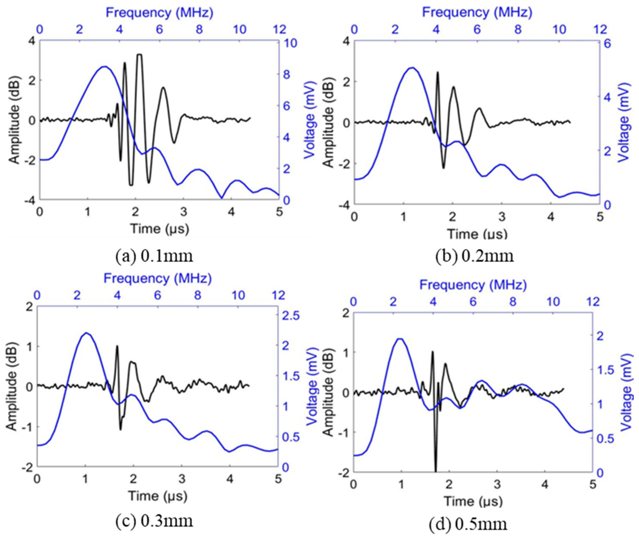
The A—scan signals corresponding to defects at various depths were extracted from the raw data matrix. These signals were then transformed into frequency spectra using the fast Fourier transform (FFT). The frequency spectra were overlaid with the original time–domain signals, as depicted in Figure 4. In this figure, the black curve represents the time–domain signal, while the blue curve represents the frequency–domain signal. The superposition of defect echoes with the surface–direct wave signal results in a distortion of the surface wave signal in the time domain and a shift in the peak position. The impact of defect echoes becomes more pronounced as the defect depth decreases. In the frequency domain, the surface wave signal with a central frequency of 5 MHz is effectively suppressed by the defect signal with a central frequency of 2 MHz. Consequently, as the defect depth increases, the spectrum gradually shifts from being dominated by a 2 MHz signal to a dual–peak signal with 2 MHz and 5 MHz as the primary components. In summary, changes in defect depth have a noticeable impact on both the time and frequency domain characteristics of the signal. Therefore, a comprehensive analysis based on the signal’s time–frequency features allows for a better assessment of defect depth.
Wavelet transform is currently one of the prevailing signal processing methods for time–frequency analysis. It builds upon and extends the localization concept of the short–time Fourier transform (STFT). The continuous wavelet transform (CWT) is particularly noteworthy for its ability to adapt the size of the time–frequency window, which outperforms the STFT’s constant window size. CWT has the capability to decompose signals of complex modes into fundamental forms, allowing for effective feature identification within the signal. It can also emphasize critical features of the signal and highlight variations in sensitive parameters. Within the realm of CWT, various wavelet basis functions are available, including the Coiflet, Cmor, Haar, and Morlet wavelets, among others. In this research, the Morlet wavelet was chosen as the basis function for CWT due to its superior capacity to capture the time–frequency characteristics of the wave signal. For a one–dimensional signal f(t), CWT can be expressed as follows, where ψ(t) represents the wavelet basis, and a and b denote the scale and translation factors, respectively:
ω ψ f a , b = 1 a + f ( t ) ψ ¯ ( t b a ) d t
ψ a , b t = 1 a ψ t b a a , b   ϵ   R . a 0
The original A—scan signals corresponding to different defects were subjected to continuous wavelet transform (CWT), and the results are shown as RGB images, as illustrated in Figure 5. This graphical representation allows for the simultaneous observation of both the time and frequency domain characteristics of the signal. The region outlined in red is the focal area of interest within the time–frequency plot. It displays crucial parameters such as the peak amplitude and time coordinates in the time domain, as well as variations in different frequency components in the spectrum.
Figure 6a displays an ultrasound B—scan signal corresponding to a specific moment in time. The red box within the image outlines the location of the pre–embedded defect. Based on the signal amplitude, a traversal and a preliminary screening of the ultrasound data within the red box were conducted to obtain the central region of the defect (highlighted in the black box within the image). Defective signals were extracted from this region in the original dataset, while non–defective signals were extracted from other regions (outside the red box). Each depth–specific defect corresponds to one category, and non–defective signals form another category, with each category consisting of 200 ultrasound A—scan signals. The batch processing of the signals using continuous wavelet transform (CWT) resulted in the generation of the original wavelet time–frequency images, as shown in Figure 6b. To improve the proportion of useful information in the time–frequency images and enhance subsequent model accuracy and training speed, an area of interest was selected within the image. Portions outside this area were excluded. The data format used for model training is illustrated in Figure 6c.
The dataset was subjected to normalization to enhance the convergence speed of the model. The dataset was divided according to the following rules: 80% of the data were selected as the training set, while the remaining 20% were allocated as the validation set. Additionally, to facilitate real–time model evaluation and fine–tuning of hyperparameters to prevent overfitting, 20% of the training set was randomly partitioned into a validation subset. The final data partitioning is summarized in Table 1.

3. Results and Discussion

3.1. Neural Network Architecture

The CNN (convolutional neural network) is one of the most extensively employed deep learning neural networks in signal analysis, with remarkable achievements in image processing and speech recognition [23,24]. It predominantly comprises three components: the input layer, feature extraction layer, and fully connected layer, as depicted in Figure 7. The input layer is utilized for inputting the training and testing data. The feature extraction layer constitutes the core of the CNN, encompassing both the convolutional and pooling layers, which collaboratively capture pivotal features from the data and learn potential patterns from the constructed datasets.
The convolutional layer filters the input data through a specified number of convolutional kernels, generating complete feature maps. This process simplifies the input data and extends them in depth. To introduce non–linearity into the model and address the issue of insufficient expressive power in linear models, enhancing the neural network’s ability to linearly separate complex features, it is common practice to incorporate activation functions following the convolution operation [25]. Commonly used activation functions include the sigmoid function, the tanh function, and the rectified linear unit (ReLU) function. The sigmoid function is primarily used in binary classification neural network structures. Tanh suffers from issues like gradient vanishing and power operations. On the other hand, the ReLU function only requires a simple check on whether the input is greater than zero, leading to faster convergence and addressing the problem of gradient vanishing. Therefore, in this study, the ReLU function is selected as the activation function. The representation of the mth feature map output from the Nth convolutional layer can be expressed as follows:
x m N = Re L U ( i = 1 M ( x i N 1 × k i m N 1 ) + b m N )
where k i m N 1 is the kernel of the Nth filter, b m N is the corresponding bias matrix, and M signifies the number of feature maps inputted from the (N − 1)–th layer.
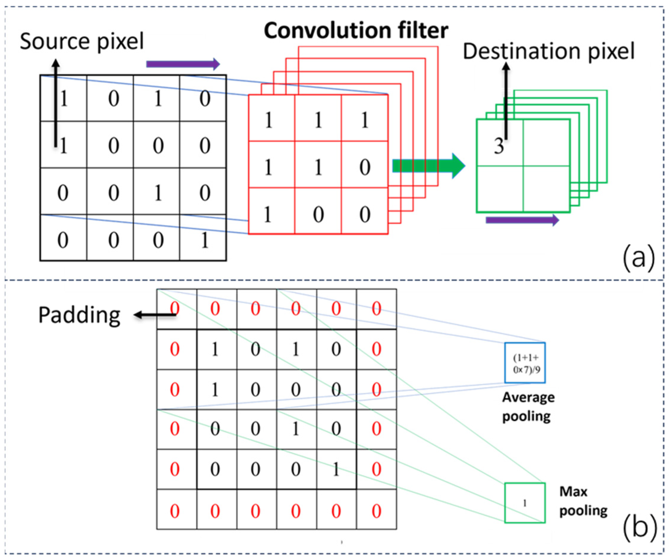
Directly using the feature map output from the convolutional layers without any processing can lead to increased computational complexity and a higher risk of overfitting during the model’s learning process. Therefore, to simplify the computational process, pooling layers are typically placed after each convolutional layer. These pooling layers down–sample the input feature maps, replacing feature information from neighboring regions with single–point data. Depending on the pooling function used, pooling can be divided into max pooling and average pooling. Average pooling computes the average of the values within the pooling range, while max pooling selects the maximum value within that range.
At the end of the CNN network, there are fully connected layers responsible for transforming the output feature maps from the previous pooling layer into feature vectors. For non–linear problems, multiple fully connected layers are often used. In a study that involves multi–classification, the output layer after the fully connected layers uses the SoftMax function to output classification labels.
The complete structure of the 2D CNN for processing ultrasonic signals is depicted in Figure 8. The input data consist of wavelet time–frequency images that have undergone crucial feature extraction and normalization. The parameters for the convolutional layers, pooling layers, and fully connected layers were optimized in accordance with the dataset size and image characteristics. The input image size used in this study is 200 × 200 × 1. Therefore, a relatively deep network is required to fully learn the data features. However, a contradiction arises as the dataset size is insufficient to support an excessively deep network structure, which could lead to overfitting and lower the model’s generalization performance.
To address this challenge, the study initially employed larger convolutional kernels and larger strides for feature extraction from the input layer. This approach allowed for rapid feature extraction while retaining image features. To mitigate overfitting, non–zero padding was used during pooling to discard certain features. Subsequent convolution was applied to the pooled feature maps using (7 × 7) convolutional kernels, which are smaller than those used in the first convolutional layer, and the number of feature maps was doubled. The resulting feature maps from the second pooling layer were further flattened, and smaller convolutional kernels with smaller strides were applied to preserve more image features. Finally, another round of pooling yielded a 256 tensor.
Two fully connected layers with 1024 neurons each were introduced to effectively address non–linear image classification. The data were ultimately transformed into probability outputs in the output layer at the bottom of the neural network, and predictions for different categories were made using the SoftMax function. The whole 2D CNN structure is shown in Figure 9, and related parameter settings is listed in Table 2.

3.2. Neural Network Optimization

To enhance the model’s generalization ability and prevent overfitting, regularization techniques were introduced to incorporate additional information into the original model. One such method is dropout, which was proposed in 2012 as an optimization technique for deep neural networks [26]. Its principle involves randomly setting a fraction of weights or outputs in hidden layers to zero during training, reducing the interdependence between nodes and, thereby, achieving the regularization of the neural network. In this study, dropout was applied before both of the two convolutional neural network layers. This process involved randomly dropping out 50% of the neurons to prevent overfitting and simultaneously improve the model’s generalization capacity. L2 regularization can be viewed as a penalty term added to the loss function, restricting certain parameters within the loss function. Given the small size of the dataset in this study, a regularization parameter was included in the loss function to further mitigate overfitting.
The selection of hyperparameters in a convolutional neural network (CNN) frequently affects the training outcomes of the model, particularly regarding the initial learning rate and batch size. Both parameters are crucial. An epoch represents the complete dataset’s single–round forward and backward propagation through the neural network. The number of samples per period might be excessive, and the computation time required for a period calculation might be too long. As a result, the data are often subdivided into several batches for training purposes.
The batch size refers to the number of samples in each batch of data. Completing one batch of sample training constitutes one iteration. Therefore, the batch size determines the direction of gradient descent in the model. When the batch size is small, the gradient direction is frequently adjusted, making it challenging to converge due to greater variability among the samples. Conversely, an excessively large batch size can result in a relatively stable gradient direction, potentially causing the model to get trapped in local optima and reducing the model accuracy.
The learning rate, on the other hand, is a hyperparameter that determines the step size during the gradient descent process, essentially dictating the size of each step during optimization. If a large initial learning rate is chosen, the optimization process may linger near the global optimum without converging to it, making it difficult to find the global optimum. Conversely, a too–small initial learning rate can slow down the rate of change of the loss function, potentially leading to overfitting and requiring more time to converge.
These considerations highlight the delicate balance required in choosing appropriate batch sizes and learning rates during the training of deep learning models to achieve effective convergence and optimal performance. In this study, the neural network preparation was conducted using TensorFlow, training was conducted with various hyperparameters, and the determination of whether the model achieved the global optimum was based on the loss function values of the training set, as illustrated in Figure 10.
From the graph, it can be observed that the three batch sizes selected in this study (16, 32, and 64) had minimal impact on the loss function. Even when the initial learning rates were set to 0.0001, 0.0002, and 0.0004, the loss function did not reach its minimum value even after 100 epochs, indicating that the model did not converge to the global optimum. However, when the initial learning rates were set to 0.001, 0.002, and 0.005, the loss function converged to its minimum value by epoch 15. Nevertheless, it is important to note that determining whether the model converges to a local or global optimum based solely on the loss function can be challenging. Therefore, further evaluation was conducted using a test set, and model performance was assessed based on the test set accuracy, as is shown in Table 3. The optimal batch size was found to be 32, and the optimal learning rate was determined to be 0.002 through a combination of loss function analysis and test set accuracy evaluation.

3.3. Depth Measurement Results

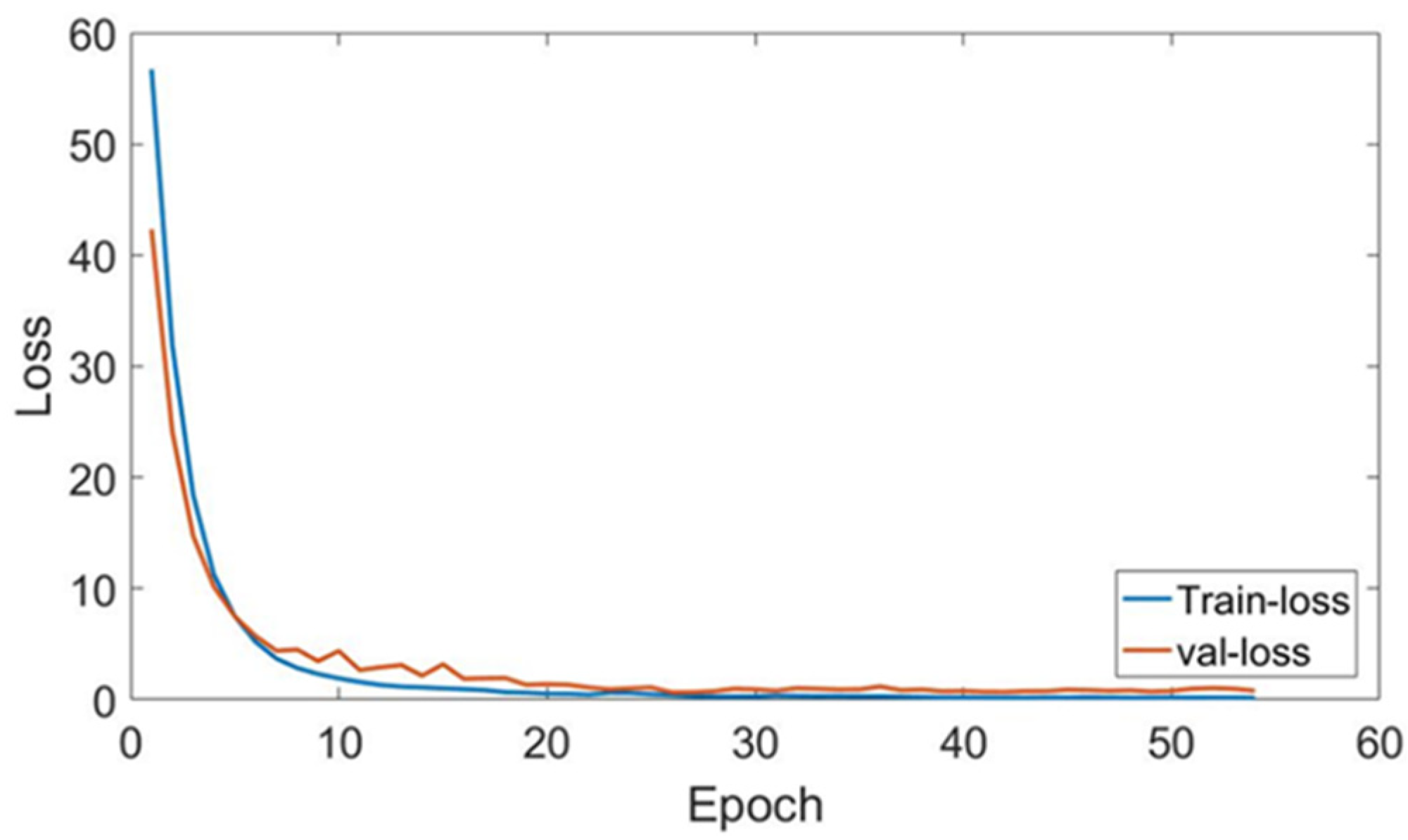
Based on the optimized hyperparameters, the convolutional neural network model was trained, and the resulting training and validation loss curves are shown in Figure 11. From the graph, it is apparent that, initially, the training loss was higher than the validation loss. Subsequently, there was a rapid gradient–descent phase, where the training loss decreased faster than the validation loss, indicating that the model converged rapidly. On the validation side, the validation loss also exhibited a descent pattern and quickly reached its minimum value.
In the end, both the validation and training sets converged to their respective minimum values, and the epochs for convergence were around 25. This suggests that, at approximately epoch 25, the model had found a local minimum during the gradient descent process. To make a further assessment, the model accuracy needs to be considered.
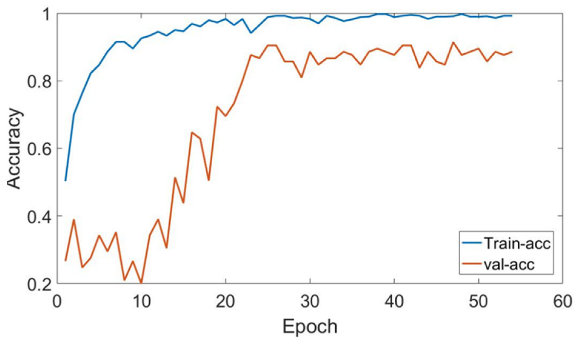
Figure 12 illustrates the accuracy curves for both the training and validation sets. The accuracy reached its peak at around epoch 25, reaching approximately 99.8% for the training set and around 91.4% for the validation set; compared to the ANN regression model [16] and similar CNN models [23] in the same field, the accuracy of our model is competitive. This confirms that, at epoch 25, the model, indeed, achieved global optimization. It is clear that our model achieves a better convergence effect in the early stage of training. Compared to similar models [15,16,17,18], the training efficiency of the model is improved after the feature extraction of the data via CWT. Early stopping was employed to terminate training when the validation accuracy ceased to improve. Continuing training beyond this point would increase the computational load and potentially lead to higher error rates in the test set.
The validation results of the model demonstrate that, at epoch 25, the loss function had reached its lowest gradient, and the model accuracy had peaked. At this stage, the convolutional neural network model was trained optimally, achieving an accuracy of 91.9% in recognizing signals from different depths of defects: 0.1 mm, 0.2 mm, 0.3 mm, 0.5 mm, and the comparisons of the depths measured using the proposed method and the designed values is shown in Figure 13; the deviation from the designed values is between −0.042 mm and +0.025 mm, and the mean deviation is ±0.037 mm.

4. Conclusions

This study aims to integrate laser ultrasonic testing methods with deep learning algorithms for the in–depth assessment of small fatigue cracks. The key innovation lies in the establishment of a 2D CNN model that incorporates input CWT spectra, enabling the intelligent monitoring and high–precision depth estimation of surface or near–surface small fatigue cracks. Through the definition of regions of interest in the original wavelet time–frequency maps based on the temporal coordinates of critical ultrasonic waveforms, the information content is enhanced. Additionally, targeted optimizations were applied to the convolutional layers, pooling layers, and fully connected layers within the neural network structure. The model’s two critical parameters, the batch size and learning rate, were further optimized through testing sets and loss functions, facilitating high–precision training under the constraints of a small dataset and effectively mitigating overfitting.
Random validation sets were employed to assess the model’s accuracy. For small cracks with a minimum depth difference of 0.1 mm, the recognition accuracy reached 91.9%, and the mean deviation of depth measured using the proposed method is ±0.037 mm. This method demonstrates the capability to assess the depth of small defects on or near surfaces effectively. Furthermore, due to the non–contact nature of laser ultrasonics, this approach holds significant potential for application in extreme environments, including the additive manufacturing, marine, and nuclear power industries.

Future Research Directions

Currently, the size of the laser ultrasonic detection system may limit the application of the present method in some scenarios with restricted detection space; we aim to design a scanning mechanism that aligns with varied detection scenarios in the future, catering to diverse detection needs. Moreover, the accuracy of our model may be enhanced through physics–based models, transfer learning, and other special optimizations, which should be further researched in the future.

Author Contributions

Conceptualization, W.X. and X.L.; methodology, W.X. and J.Z.; investigation, Q.F., J.C. and L.J.; writing—original draft preparation, Q.F. and J.C.; writing—review and editing, J.Z. and J.Y.; supervision, H.D.; project administration, J.Y. and H.D. All authors have read and agreed to the published version of the manuscript.

Funding

This research was funded by the National Key Research and Development Project of China, grant number 2018YFB1106100.

Institutional Review Board Statement

Not applicable.

Informed Consent Statement

Not applicable.

Data Availability Statement

The data presented in this study are available on request from the corresponding author.

Conflicts of Interest

The authors declare no conflict of interest.

References

  1. García-Martínez, M.; del Hoyo Gordillo, J.C.; Valles González, M.P.; Pastor Muro, A.; González Caballero, B. Failure study of an aircraft engine high pressure turbine (HPT) first stage blade. Eng. Fail. Anal. 2023, 149, 107251. [Google Scholar] [CrossRef]
  2. Qin, C.; He, S.; Zhong, L.; Feng, W.; Pang, J.; Li, Q.; He, W. Fracture failure analysis of pressure gauge bolt on fuel gas system of offshore platform. Eng. Fail. Anal. 2020, 117, 104959. [Google Scholar] [CrossRef]
  3. Zobaer Shah, Q.M.; Chowdhury, M.A.; Kowser, M.A. The aspect of the corrosion pitting with fretting fatigue on Aluminum Alloy: A nuclear reactor safety or an aerospace structural failure phenomenon. Results Eng. 2022, 15, 100483. [Google Scholar] [CrossRef]
  4. Wu, W.P.; Li, Z.Z.; Chu, X. Peridynamics study on crack propagation and failure behavior in Ni/Ni3Al bi-material structure. Compos. Struct. 2023, 323, 117453. [Google Scholar] [CrossRef]
  5. Oshima, S.; Higuchi, R.; Kobayashi, S. Experimental characterization of cracking behavior initiating from microdefects in cross-ply CFRP laminates. Eng. Fract. Mech. 2023, 281, 109116. [Google Scholar] [CrossRef]
  6. Kenderian, S.; Djordjevic, B.B.; Green, R.E. Point and line source laser generation of ultrasound for inspection of internal and surface flaws in rail and structural materials. Res. Nondestruct. Eval. 2001, 13, 189–200. [Google Scholar] [CrossRef]
  7. Liao, D.; Yin, M.; Yi, J.; Zhong, M.; Wu, N. A nondestructive testing method for detecting surface defects of Si3N4-Bearing cylindrical rollers based on an optimized convolutional neural network. Ceram. Int. 2022, 48, 31299–31308. [Google Scholar] [CrossRef]
  8. He, J.; Liu, X.; Cheng, Q.; Yang, S.; Li, M. Quantitative detection of surface defect using laser-generated Rayleigh wave with broadband local wavenumber estimation. Ultrasonics 2023, 132, 106983. [Google Scholar] [CrossRef]
  9. Zhang, Z.; Zhao, J.; Pan, Y. Surface circular-arc defects interacted by laser-generated Rayleigh wave. Ultrasonics 2020, 103, 106085. [Google Scholar] [CrossRef] [PubMed]
  10. Masserey, B.; Fromme, P. Surface defect detection in stiffened plate structures using Rayleigh-like waves. NDT E Int. 2009, 42, 564–572. [Google Scholar]
  11. Cheng, W.; Sun, H.H.; Wan, L.S.; Fan, Z.; Tan, K.H. Corrosion damage detection in reinforced concrete using Rayleigh wave-based method. Cement Concrete Comp. 2023, 143, 105253. [Google Scholar] [CrossRef]
  12. Thring, C.B.; Fan, Y.; Edwards, R.S. Focused Rayleigh wave EMAT for characterization of surface-breaking defects. NDT E Int. 2016, 81, 20–27. [Google Scholar]
  13. Chen, H.; Zhang, G.; Fan, D.; Fang, L.; Huang, L. Nonlinear Lamb wave analysis for microdefect identification in mechanical structural health assessment. Measurement 2020, 164, 108026. [Google Scholar] [CrossRef]
  14. Dehghan-Niri, E.; Al-Beer, H. Phase-space topography characterization of nonlinear ultrasound waveforms. Ultrasonics 2018, 84, 446–458. [Google Scholar] [CrossRef]
  15. Fu, L.L.; Yang, J.S.; Li, S.; Luo, H.; Wu, J.H. Artificial neural network-based damage detection of composite material using laser ultrasonic technology. Measurement 2023, 220, 113435. [Google Scholar] [CrossRef]
  16. Chen, D.; Zhou, Y.; Wang, W.; Zhang, Y.; Deng, Y. Ultrasonic signal classification and porosity testing for CFRP materials via artificial neural network. Mater. Today Commun. 2022, 30, 103021. [Google Scholar] [CrossRef]
  17. Yang, Z.; Yang, H.; Tian, T.; Deng, D.; Hu, M.; Ma, J.; Gao, D.; Zhang, J.; Ma, S.; Yang, L.; et al. A review on guided-ultrasonic-wave-based structural health monitoring: From fundamental theory to machine learning techniques. Ultrasonics 2023, 133, 107014. [Google Scholar] [CrossRef] [PubMed]
  18. Amiri, N.; Farrahi, G.H.; Kashyzadeh, K.R.; Chizari, M. Applications of ultrasonic testing and machine learning methods to predict the static & fatigue behavior of spot-welded joints. J. Manuf. Process 2020, 52, 26–34. [Google Scholar]
  19. Czarnecki, S.; Shariq, M.; Nikoo, M.; Sadowski, Ł. An intelligent model for the prediction of the compressive strength of cementitious composites with ground granulated blast furnace slag based on ultrasonic pulse velocity measurements. Measurement 2021, 172, 108951. [Google Scholar] [CrossRef]
  20. Tenza-Abril, A.J.; Villacampa, Y.; Solak, A.M.; Baeza-Brotons, F. Prediction and sensitivity analysis of compressive strength in segregated lightweight concrete based on artificial neural network using ultrasonic pulse velocity. Constr. Build. Mater. 2018, 189, 1173–1183. [Google Scholar] [CrossRef]
  21. Wang, F.; Song, G. Looseness detection in cup-lock scaffolds using percussion-based method. Automat. Constr. 2020, 118, 103266. [Google Scholar] [CrossRef]
  22. Wang, F.; Mobiny, A.; Van Nguyen, H.; Song, G. If structure can exclaim: A novel robotic-assisted percussion method for spatial bolt-ball joint looseness detection. Struct. Health Monit. 2020, 20, 1597–1608. [Google Scholar] [CrossRef]
  23. Valizadeh, M.; Wolff, S.J. Convolutional Neural Network applications in additive manufacturing: A review. Adv. Indust. Manufact. Eng. 2022, 4, 100072. [Google Scholar] [CrossRef]
  24. Hema, C.; Garcia Marquez, F.P. Emotional speech Recognition using CNN and Deep learning techniques. Appl. Acoust. 2023, 211, 109492. [Google Scholar] [CrossRef]
  25. Habib, G.; Qureshi, S. Optimization and acceleration of convolutional neural networks: A survey. J. King Saud Univ. Com. Infor. Sci. 2022, 34, 4244–4268. [Google Scholar] [CrossRef]
  26. Srivastava, N.; Hinton, G.; Krizhevsky, A.; Sutskever, I.; Salakhutdinov, R. Dropout: A simple way to prevent neural networks from overfitting. J. Mach. Learn. Res. 2014, 15, 1929–1958. [Google Scholar]
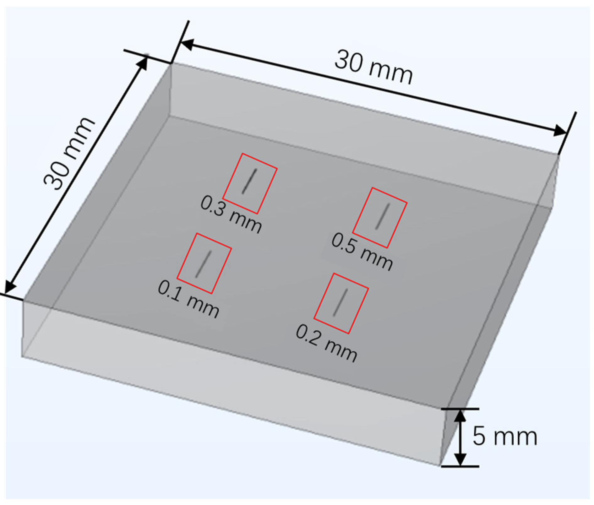
Figure 1. Schematic diagram for the sample.
Applsci 13 11559 g001
Figure 2. The testing system: (a) schematic diagram; (b) photograph of the real product.
Applsci 13 11559 g002
Figure 3. The laser ultrasonic data acquisition system: (a) schematic diagram, (b) scanning strategy, (c) 3D data storage.
Applsci 13 11559 g003
Figure 4. The ultrasonic A—scan signal and its spectra of different defect depths: (a) 0.1 mm, (b) 0.2 mm, (c) 0.3 mm, and (d) 0.5 mm.
Applsci 13 11559 g004
Figure 5. The wavelet time–frequency plots of different defect depths: (a) 0.1 mm, (b) 0.2 mm, (c) 0.3 mm, and (d) 0.5 mm.
Applsci 13 11559 g005
Figure 6. The dataset preprocessing process: (a) the B—scan extracted from the raw data, (b) the wavelet transform of the A—scan, (c) an interesting region of the time–frequency image.
Applsci 13 11559 g006
Figure 7. The typical architecture of a CNN.
Applsci 13 11559 g007
Figure 8. The principles of feature extraction: (a) convolutional layer, (b) pooling layer.
Applsci 13 11559 g008
Figure 9. The 2D CNN structure incorporated with inputted CWT spectra from raw signals.
Applsci 13 11559 g009
Figure 10. The train loss for different batch sizes and learning rates: (a) batch size 16, (b) batch size 32, and (c) batch size 64.
Applsci 13 11559 g010
Figure 11. The training loss of the test set and validation set.
Applsci 13 11559 g011
Figure 12. The accuracy of the test set and validation set.
Applsci 13 11559 g012
Figure 13. The comparison of the depths measured using the proposed method and the designed values: (a) the comparison results, (b) the deviations from the designed values.
Applsci 13 11559 g013
Table 1. Dataset partitioning.
Type0.1 mm0.2 mm0.3 mm0.5 mmNo Defect
Training set140140140140140
Test set4040404040
Validation set2020202020
Table 2. The parameter settings of 2D CNN.
LayerTypeParameter Settings
L1ConvFilter number = 64, kernel size = 11 × 11, stride = 4, activation = ’ReLU’, padding = ’same’
L2Max-poolingKernel size = 3 × 3, stride = 4, padding = ’invalid’
L3ConvFilter number = 128, kernel size = 7 × 7, stride = 4, activation = ’ReLU’, padding = ’same’
L4Max-poolingKernel size = 3 × 3, stride = 2, padding = ’valid’
L5ConvFilter number = 256, kernel size = 3 × 3, stride = 1, activation = ’ReLU’, padding = ’same’
L6Max-poolingKernel size = 3 × 3, stride = 2, padding = ’valid’
L7FCUnits = 1024, activation = ’ReLU’
L8FCUnits = 1024, activation = ’ReLU’
L9FCUnits = 5, activation = ’Softmax’
Table 3. The test set accuracy for different batch sizes and learning rates.
Learning Rate0.010.0050.0010.0020.00040.00020.0001
Batch Size
6488.7%87.8%88.2%90.5%81.9%77.8%86.0%
3288.7%86.9%88.7%91.9%83.7%83.7%82.8%
1687.8%83.7%88.7%86.0%73.8%84.2%80.1%
Disclaimer/Publisher’s Note: The statements, opinions and data contained in all publications are solely those of the individual author(s) and contributor(s) and not of MDPI and/or the editor(s). MDPI and/or the editor(s) disclaim responsibility for any injury to people or property resulting from any ideas, methods, instructions or products referred to in the content.