Oxygen Demand Forecasting and Optimal Scheduling of the Oxygen Gas Systems in Iron- and Steel-Making Enterprises

Abstract

Due to the imbalance between the supply and demand of oxygen, the oxygen systems of iron- and steel-making enterprises in China have problems with high oxygen emissions and high pressure in the pipelines, resulting in the energy consumption of oxygen production being high. To reduce the energy consumption of oxygen systems, this study took a large-scale iron- and steel-making enterprise as a case study and developed a two-stage forecasting and scheduling model. The novel aspect and progressiveness of this work are as follows: First, an oxygen demand forecasting model was developed based on the backpropagation neural network with genetic algorithm optimization (GABP) and is driven only by historical data. Compared with some complex models in the literature, although the accuracy of this model has been reduced, the model does not need to consider production plans for other process steps, making it more practical and feasible. Second, different from the existing literature, an oxygen production scheduling model was developed for load-variable ASUs with an internal compression process, and both the oxygen emissions and pipeline pressure are included in the objective function. The case study showed that based on the oxygen demand forecast and optimal scheduling, the oxygen emissions and pipeline pressure in the studied iron- and steel-making enterprise can be significantly reduced, thereby achieving considerable energy-saving effects and economic benefits. Specifically, the following conclusions were obtained: (1) For the oxygen demand forecast, the prediction accuracy of the GABP model was better than that of the ARIMA model. The average MAPE of the 12 sets of data of the ARIMA and GABP models was 23.8% and 20.2%, respectively. (2) By comparing the scheduling results and the field data, it was found that after scheduling, the amount of oxygen emissions decreased by 6.32%, the pipeline pressure decreased by 0.61%, and the energy consumption of oxygen compression decreased by 1.6%. Considering both the oxygen emission loss and the energy consumption of oxygen compression, the total power consumption of the studied oxygen system was reduced by 1.38%, resulting in electricity cost savings of approximately 9.03 million RMB per year.

1. Introduction

China is a major steel producer, and its crude steel production accounts for more than 50% of global crude steel production [1]. Steel production capacity is the embodiment of a country’s industrial strength, but high output also means high energy consumption. The energy consumption of the steel industry accounts for approximately 15% of China’s total energy consumption [2]. Blast furnace iron-making and converter steel-making require a large amount of oxygen, which is mainly produced by separating air in an air separation unit (ASU) using a cryogenic rectification method. Most of the iron- and steel-making enterprises in China have captive oxygen plants, which are equipped with several large-scale ASUs. The oxygen systems of iron- and steel-making enterprises are mainly composed of ASUs, oxygen compressors, and high-pressure storage vessels.

Oxygen systems are energy-extensive and a large power consumer in iron and steel production enterprises because the separation process of air and the pressure delivery process of oxygen consume a lot of electric energy. In China, oxygen systems often have an imbalance between supply and demand. On the oxygen supply side, ASUs have the characteristic of stable production due to the characteristics of the equipment, and their output is relatively stable. However, on the oxygen demand side, affected by the production rhythm, the oxygen demand fluctuates greatly. At present, ASUs, blast furnaces, and converters tend to be very large, and the amount of equipment decreases when the steel output remains unchanged. This further aggravates the imbalance between the supply and demand of oxygen systems, resulting in a waste of resources and energy.

To cope with the imbalance between supply and demand, the main scheduling means that can be adopted in oxygen systems are gas storage by high-pressure spherical vessels and load adjustment of ASUs. High-pressure spherical vessels can passively buffer the fluctuation of oxygen demand, while load adjustment of ASUs can be used as an active means to alleviate the fluctuation of oxygen demand, but the oxygen demand needs to be forecasted in advance. Oxygen demand forecasting and ASU variable-load operation are relatively complex. In the absence of a decision-making support system, it is difficult to predict and schedule oxygen systems via human judgment. As a compromise, at present, on-site workers generally adopt the practice of oxygen supply exceeding demand to ensure production safety, but the price paid is that the pressure of the oxygen pipeline is high and oxygen is often emitted, which results in high energy consumption for oxygen delivery and causes release loss. The optimized production and reasonable transportation of oxygen can effectively reduce the total energy consumption of steel production and play a positive role in promoting the early realization of carbon peaks in the steel industry. Therefore, it is necessary to establish a demand forecasting and optimal scheduling model for oxygen systems [3,4,5].

In terms of oxygen demand forecasting, most forecasting models are based on predicting the production rhythm of basic oxygen furnaces (BOFs) [6,7,8,9]. Ruuska et al. [10] presented a new model that describes the relationship between input variables such as blast temperature and blast composition and the output variable, namely, the tapped temperature of the steel. Daniela et al. [11] presented a study on the dynamic modeling and simulation of BOF operation with potential applications for process control and optimization in the steel industry. Peng et al. [12] presented a study on a novel modeling method based on support vector domain description and LS-SVM for steel-making processes. Jiang et al. [13] presented a Gaussian process-based hybrid model for predicting oxygen consumption in the converter steel-making process. Zhou et al. [14] proposed two novel long-term prediction methods using MOGPR-based prediction enhancement to solve this industrial problem by learning from historical data and production plans.

In terms of oxygen production scheduling, Han et al. [15] proposed an oxygen system scheduling model that considers power costs, using a particle swarm optimization algorithm to solve the model, and validated the model’s effectiveness through actual field data. Zhang et al. [3] studied oxygen balance and scheduling under blast furnace shutdown conditions and established a scheduling model for air separation startup and shutdown based on mixed integer linear programming [16]. Xu et al. [17] proposed a production scheduling optimization model that was built to minimize the oxygen demand fluctuation and the penalty cost of casts’ starting time. Zhang et al. [18] developed a scheduling model for an oxygen system, which was tested on actual production data. Moreover, to improve the limitation of current ASU models with a single type of load adjustment, Zhang et al. [19] established a general framework for modeling ASU scheduling to unify multiple load-adjustment types and applied it to an oxygen system scheduling model. Liu et al. [20] presented a study on a novel dynamic operation optimization method based on multi-objective deep reinforcement learning for steel-making processes.

Relative to forecasting and scheduling models, few studies have investigated a two-stage model containing both forecasting and scheduling. Han et al. [21] proposed a two-stage predictive scheduling method, in which a predictive model based on granular computing (GrC) and a mixed integer optimization model were established in the prediction and scheduling stages, respectively. The application results showed the accuracy and practicality of the method. Jiang et al. [22] investigated the problem of optimal oxygen distribution with flexible demands under uncertainty and proposed a two-stage robust optimization model with a budget-based uncertainty set that protected the initial distribution policy with low conservatism. Zhang et al. [23] presented a two-stage distributionally robust integrated scheduling approach for oxygen distribution and continuous casting processes in steel-making enterprises.

With the rapid development of the industrial Internet and intelligent manufacturing technology, digital twins will gradually become popular in the industry. It has become possible to carry out predictions and analyses based on big data and machine learning and drive the physical world with optimal results. This study took a large-scale iron- and steel-making enterprise as a study case and developed a two-stage forecasting and scheduling model for reducing the energy consumption of its oxygen system. The novel aspect and progressiveness of this work are as follows: First, the oxygen demand forecasting model was developed based on the backpropagation neural network with genetic algorithm optimization (GABP) and is driven only by historical data. Compared with research in the literature, the accuracy of this model has been reduced, but the model does not need to consider production plans for other process steps, making it more practical and feasible. Second, different from the existing literature, an oxygen production scheduling model was developed for load-variable ASUs with an internal compression process, and both the oxygen emissions and pipeline pressure are included in the objective function. Moreover, the accuracy of the forecast model and the energy-saving effect of the scheduling model were verified through field data.

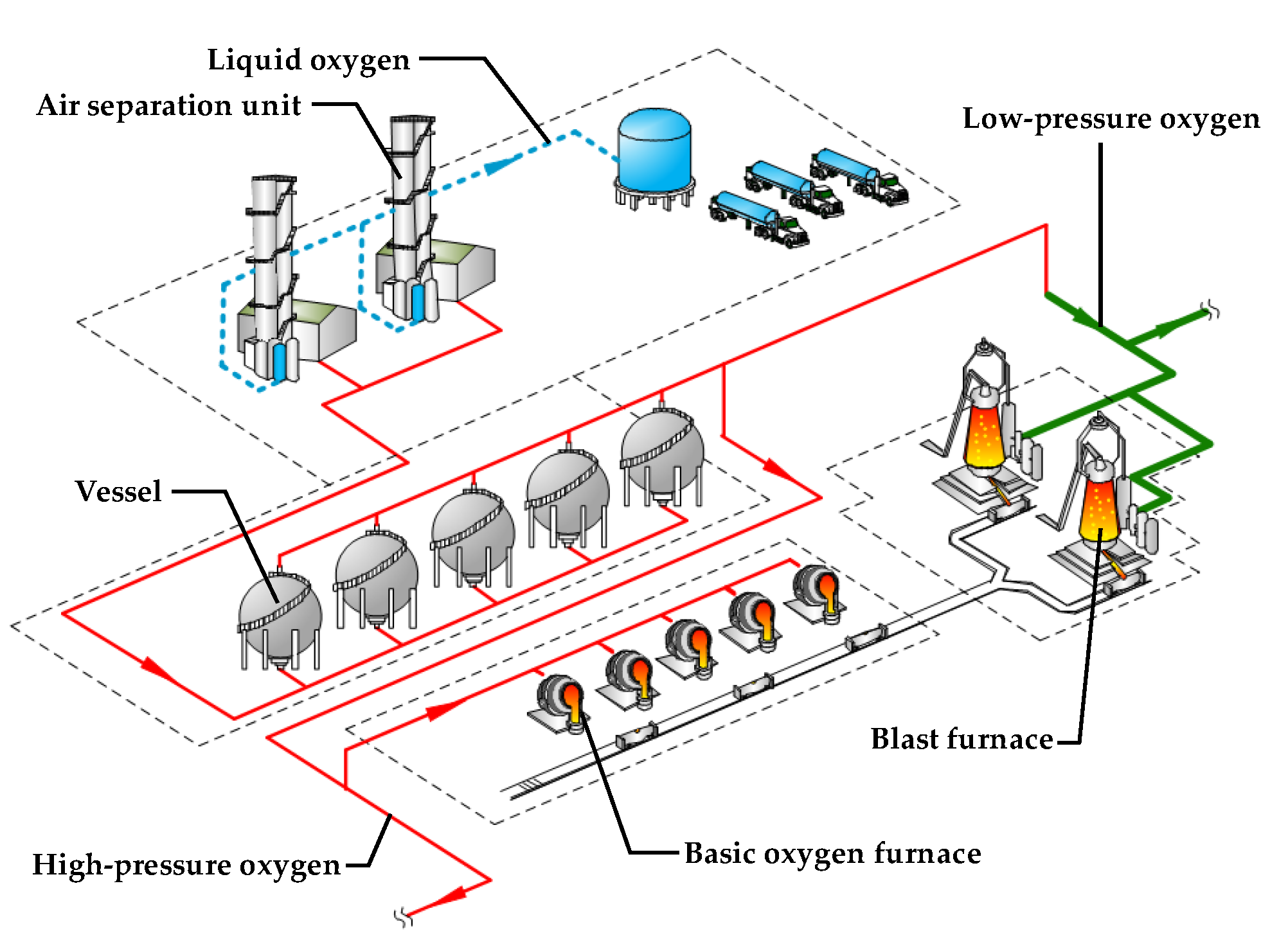
2. Case Descriptions

As shown in Figure 1, the case study involved the oxygen system of a large-scale iron- and steel-making enterprise. In this oxygen system, the oxygen production equipment comprise two sets of large-scale load-variable ASUs with an internal compression process, and their relevant parameters are shown in

Table 1. Parameters of the ASUs.

ASU	Design Output (m3·h−1)	Max. Output (m3·h−1)	Min. Output (m3·h−1)	Initial Output (m3·h−1)	Load Variation Rate (m3·h−2)
1#	75,000	78,750	60,000	70,500	11,250
2#	75,000	78,750	60,000	71,000	11,250

. The oxygen system is also equipped with five spherical vessels as buffer equipment, and its related parameters are shown in

Table 2. Parameters of the oxygen vessels.

Vessel	Total Capacity (m3)	Max. Pressure Pmax (MPa)	Min. Pressure Pmin (MPa)
V1~V5	4000	3.0	1.6

. The main users of oxygen are five converters and two blast furnaces, among which the converters have the characteristics of batch smelting, and the time interval between two smelting cycles has great uncertainty, which is the main reason for the fluctuation of oxygen demand. Meanwhile, the blast furnaces are in continuous production, and the oxygen demand is relatively stable.

For research and analysis, a large amount of field data (collected every 2 min) was collected. The oxygen demands, ASU outputs, and pipeline pressure under normal production conditions (no blast furnace shutdown, converter maintenance, etc.) for four consecutive days were selected as the sample data to be analyzed.

3. Oxygen Demand Forecasting Model

The total amount of oxygen used in multi-converter steel-making not only depends on linear factors that change over time but also on nonlinear factors such as the randomness of manual operation and the random overlapping of oxygen consumption by multiple converters. The autoregressive integrated moving average (ARIMA) model [24] can predict future data based on existing time series data and is suitable for processing time series data with strong linear correlation. The GABP model can learn historical data through neural network training. When the time series data have a strong nonlinear correlation, the GABP model has strong adaptability [25]. Therefore, for comparison purposes, both the ARIMA and GABP models were selected to forecast the oxygen demand.

3.1. The ARIMA Model

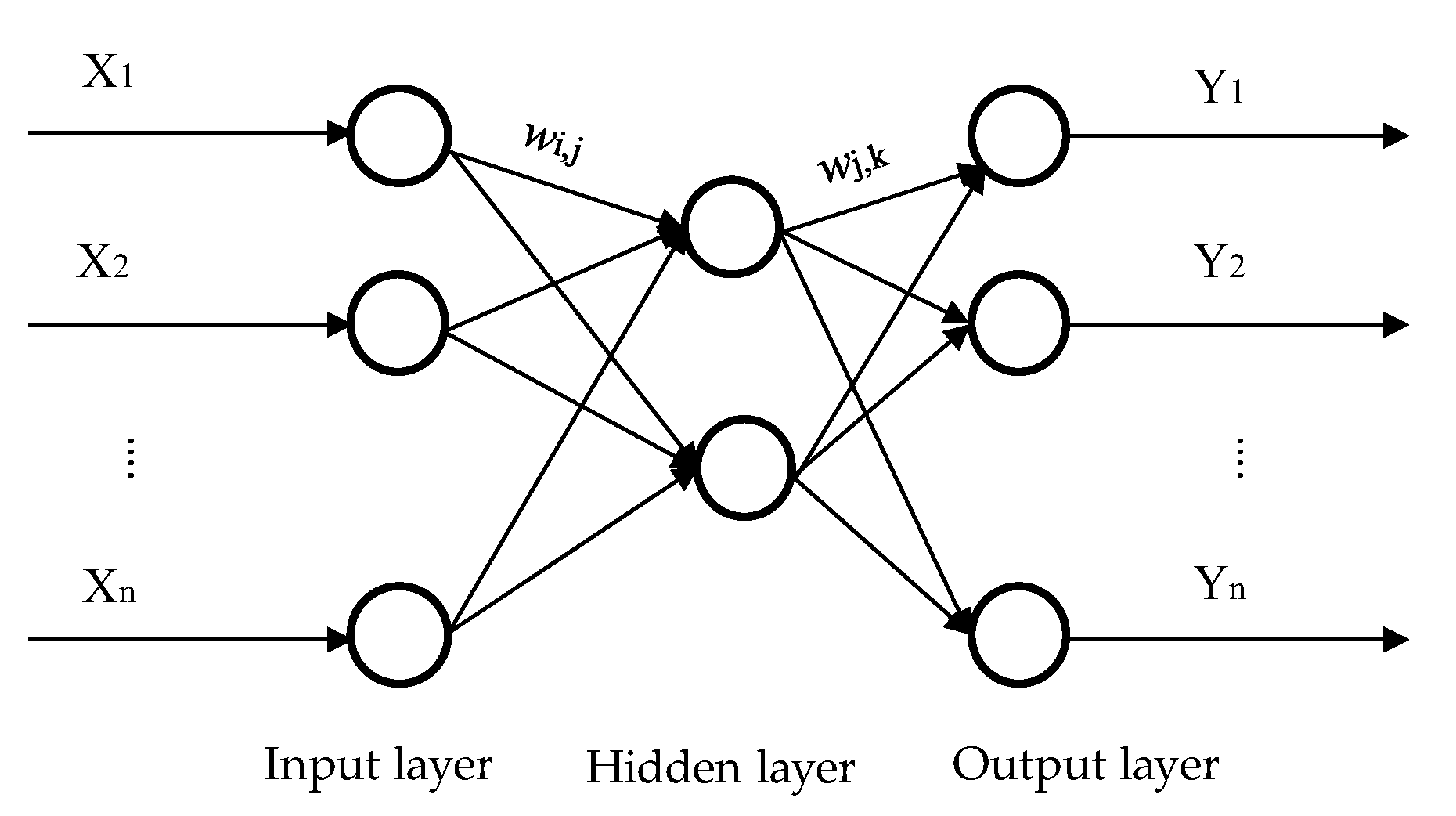
For the non-stationary sequence analysis, smoothing (difference) processing was performed first, and then the time series data after the stabilization (difference) were modeled and analyzed. For the d-order difference, the expression is:

$${\nabla }^d{x}_t={\nabla }^{\mathrm{d}-1}{x}_t-{\nabla }^{\mathrm{d}-1}{x}_{t-1}$$

(1)

The general mathematical expression of the $\mathrm{A}\mathrm{R}\mathrm{I}\mathrm{M}\mathrm{A}(p,d,q)$ model is:

$$\left(1-\sum _{i=1}^p{\varphi }_i{L}^i\right)(1-L{)}^d{X}_t=\left(1+\sum _{i=1}^q{\theta }_i{L}^i\right){\epsilon }_t$$

(2)

where d is the difference order, p is the autoregressive order, q is the moving average order, L is the lag factor, $\varphi$ is the autoregressive factor corresponding to the p-order, L is the lag factor, $X_t$ is the observed value at the time t during the random process, $\theta$ is the moving average coefficient corresponding to q-order, and $\epsilon$ is the term of random error.

3.2. The GABP Model

As shown in Figure 2, the BP neural network is a kind of feed-forward network, and the network structure is composed of an input layer, a hidden layer, and an output layer. X₁, X₂, …, X_n are the input values, Y₁, Y₂, …, Y_n are the prediction values, and w_i,j and w_j,k are the weights of the BP neural network. The neural network utilizes the network structure and parameters to perform nonlinear learning on the data samples and stores the learning information in the network weights and thresholds, thereby memorizing the development law of the data sequence and realizing the forecast of future data sequences. However, the randomness of parameter selection in the initial training of the neural network is strong, and the correction of weights and thresholds tends to fall into a local optimal solution, resulting in a forecast error greater than the expected error. This optimization defect can be addressed by introducing a GA.

GA is an algorithm that simulates the natural evolution process of organisms to search for the optimal solution. It has the advantages of strong parallel computing ability and strong adaptability [26]. GA adopts the individual to express the value to be corrected and uses the error binary norm between the forecast output and the actual expected number as the population fitness value. The smaller fitness value is used as the candidate individual, and then a series of crossover and mutations are performed. After reaching the preset evolutionary algebra, the remaining individual is the optimal individual, and then the initial training parameters of the neural network are obtained.

4. Oxygen Scheduling Model

According to the actual situation of the oxygen system, the scheduling model adopts the following simplifications and assumptions: (1) The scheduling objects are gas spherical vessels and ASUs operated with variable loads; (2) in the load change process of ASUs, both nitrogen and argon products meet the demand, so the constraints for nitrogen and argon are not included; (3) during the scheduling process, no failures occur in the ASUs, blast furnace, or converter.

4.1. Object Function

The production of oxygen by ASUs requires energy, so the oxygen emissions will directly cause energy waste. Moreover, the higher the pressure of the oxygen pipeline, the greater the energy consumed to compress a unit of oxygen. Therefore, the scheduling objective is to minimize both the oxygen emissions and the pipeline pressure, and the objective function is as follows:

$$Z=\mathrm{Min}(\sum _{t=1}^{N}0.5E_t+\sum _{t=1}^{N}0.5P_t)$$

(3)

where $Z$ is the optimization objective, $E_t$ is the amount of oxygen emissions at time t, $P_t$ is the pipeline pressure at time t, and $N$ is the number of scheduling periods.

4.2. Constraint Conditions

4.2.1. Constraints for the ASUs

In actual operation, the output of an ASU can be adjusted at a limited rate within a certain range, which is shown in Table 1, and the constraint equation is as follows:

$$Ag{o}_i^{t-1}-b_i\mathsf{\Delta }t<Ag{o}_i^t<Ag{o}_i^{t-1}+b_i\mathsf{\Delta }t$$

(4)

where $Ag{o}_i^{t-1} \mathrm{a}\mathrm{n}\mathrm{d} Ag{o}_i^t$ are the ASU outputs at time $t-1$ and $t$, respectively, $b_i$ is the maximum value of the load change rate of the ASU, and $\Delta t$ is the step length of the period.

$$Ag{o}_{i_{\mathrm{m}\mathrm{i}\mathrm{n}}}<Ag{o}_i^t<Ag{o}_{i_{\mathrm{m}\mathrm{a}\mathrm{x}}}$$

(5)

where $Ag{o}_{i_{\mathrm{m}\mathrm{i}\mathrm{n}}}$ and $Ag{o}_{i_{\mathrm{m}\mathrm{a}\mathrm{x}}}$ are the minimum and maximum oxygen outputs of the ASU, respectively.

4.2.2. Constraints for the Pipeline Pressure

The pressure $P_t$ of the gas storage vessels and the pipeline is restricted by the lower-pressure limit, $P_{\mathrm{m}\mathrm{i}\mathrm{n}}$, and the upper-pressure limit, $P_{\mathrm{m}\mathrm{a}\mathrm{x}}$. The relevant parameters are shown in Table 2, and the constraint equation is as follows:

$$P_{\mathrm{m}\mathrm{i}\mathrm{n}}<P_t<P_{\mathrm{m}\mathrm{a}\mathrm{x}}$$

(6)

4.2.3. Mass Conservation Constraints for the Oxygen System

The oxygen system needs to satisfy mass conservation, that is, the sum of the total oxygen production of the ASUs minus the oxygen emissions, and the oxygen demand is equal to the oxygen storage capacity of the buffer equipment. The constraint equation is as follows:

$$\sum _{i=1}^{2}Ag{o}_{i,t}-E_t-D_t=\frac{0.0224(P_t-P_{t-1}){\sum }_{j=1}^5{V}_j}{RT\mathsf{\Delta }t}$$

(7)

where $D_t$ is the oxygen demand of the enterprise, $V_j$ is the total volume of the gas storage vessels, $R$ is the gas constant, and $T$ is the environmental temperature.

5. Results and Discussion

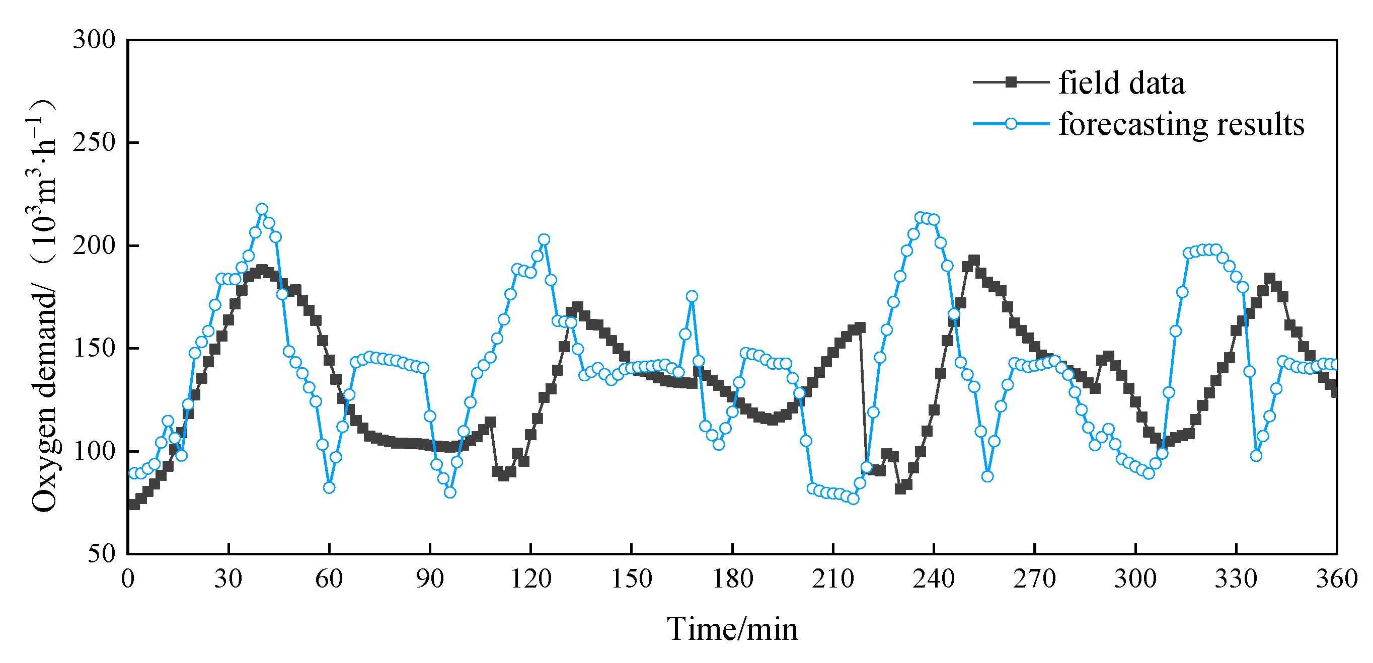
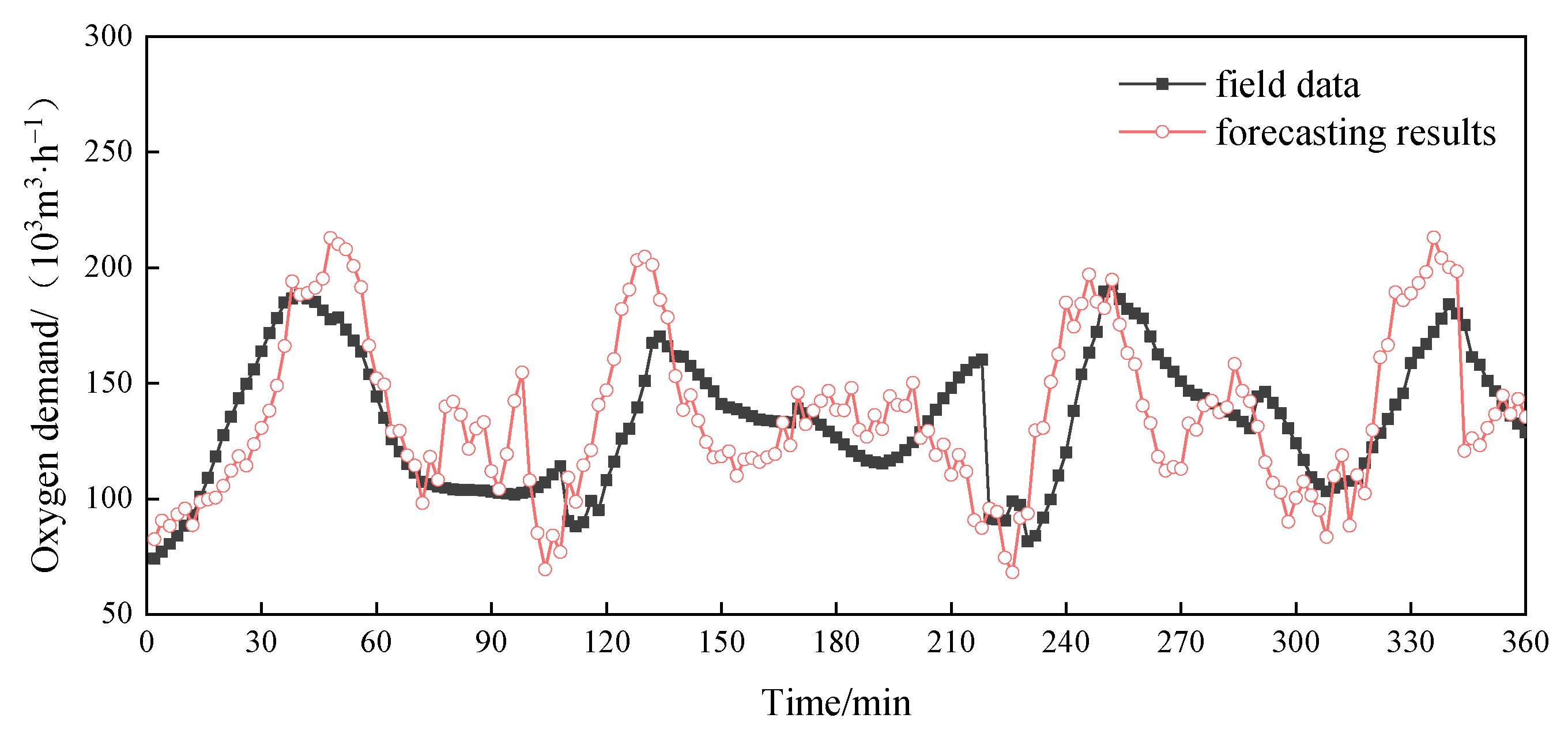
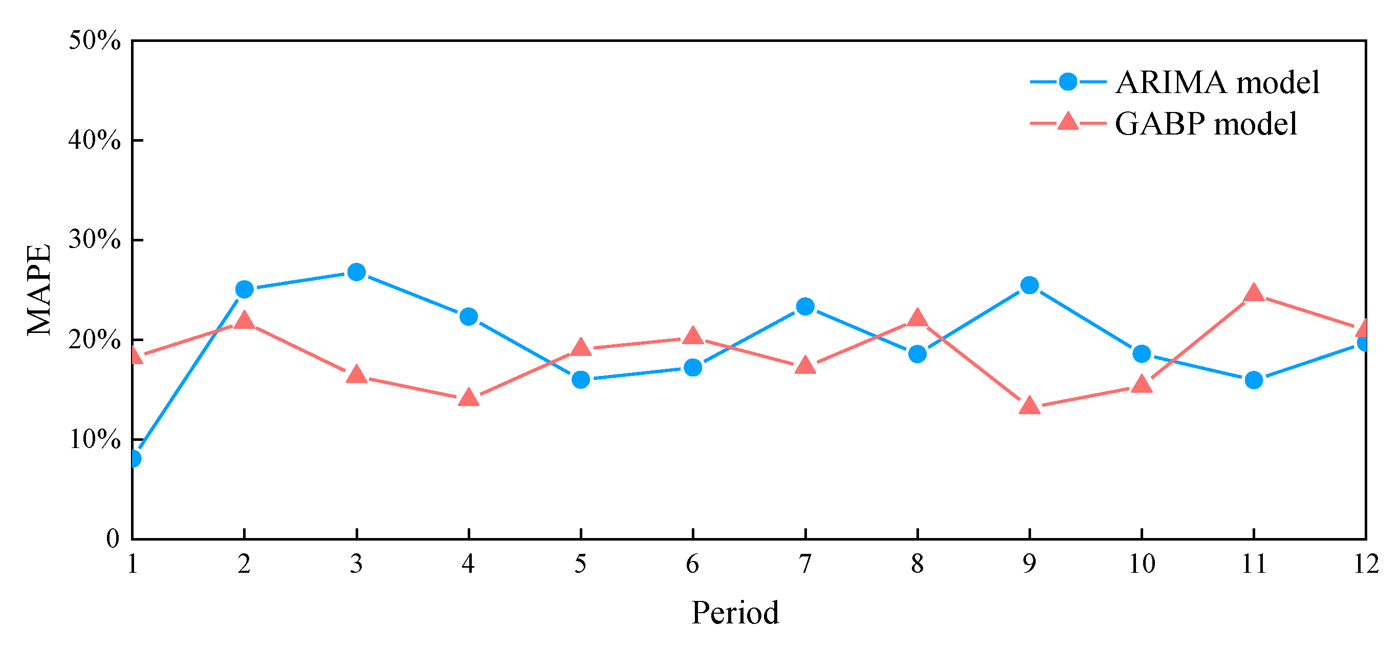
5.1. Analysis of the Forecasting Results of the Oxygen Demand

The collected field data were divided into 12 groups for forecasting and verification. Each group of data contained 165 data points, of which the first 150 data points were used as input data for forecasting, and the last 15 data points as verification data for the forecast results. This is equivalent to forecasting the oxygen demand for the next half an hour based on 5 h of historical data. In addition, some of the field data are provided in

Table 3. Some of the field data of the oxygen demand.

No.	Demand (m3·h−1)	No.	Demand (m3·h−1)	No.	Demand (m3·h−1)	No.	Demand (m3·h−1)
1	112,215	11	141,537	21	101,184	31	151,993
2	132,765	12	145,090	22	100,658	32	192,764
3	138,769	13	140,438	23	78,983	33	165,735
4	139,979	14	142,175	24	79,322	34	174,441
5	146,382	15	141,378	25	86,324	35	199,188
6	183,921	16	131,942	26	84,529	36	198,568
7	203,641	17	122,900	27	120,073	37	176,028
8	172,899	18	82,587	28	158,378	38	147,128
9	158,281	19	115,577	29	160,183	39	144,668
10	155,339	20	99,487	30	148,698	40	149,441

for a better understanding of the input and output of the models.

First, the ARIMA model forecast was performed on the data, and ARIMA (2,1,5) was obtained as the optimal model for time series prediction. Second, the GABP model forecast was performed on the data, in which the GA optimization algorithm was set as follows: The genetic algebra was 100, the population size was 50, the crossover probability was 0.4, the mutation probability was 0.3, the number of nodes in the hidden layer of the BP neural network was 18, the activation function of the hidden layer was a tansig function, the excitation function of the output layer was a purelin function, the learning rate was 0.05, the target error precision was 0.01, and the number of network iteration steps was 5000.

The forecasting was performed using MATLAB 9.6 (R2019a) software, and the results of the ARIMA and GABP models are shown in Figure 3 and Figure 4, respectively.

When comparing Figure 3 and Figure 4, it can be seen that both the ARIMA and GABP models can forecast the changing trend of the oxygen demand, but the GABP model performed better than the ARIMA model in terms of coincidence with the field data. To quantificationally compare the forecast accuracy of the two models, the mean absolute percentage error (MAPE) of each of the 12 sets of data was calculated and is shown in Figure 5. The calculation results show that the average MAPE values of the 12 sets of data of the ARIMA and GABP models were 23.8% and 20.2%, respectively. Therefore, the prediction accuracy of the GABP model is better than that of the ARIMA model.

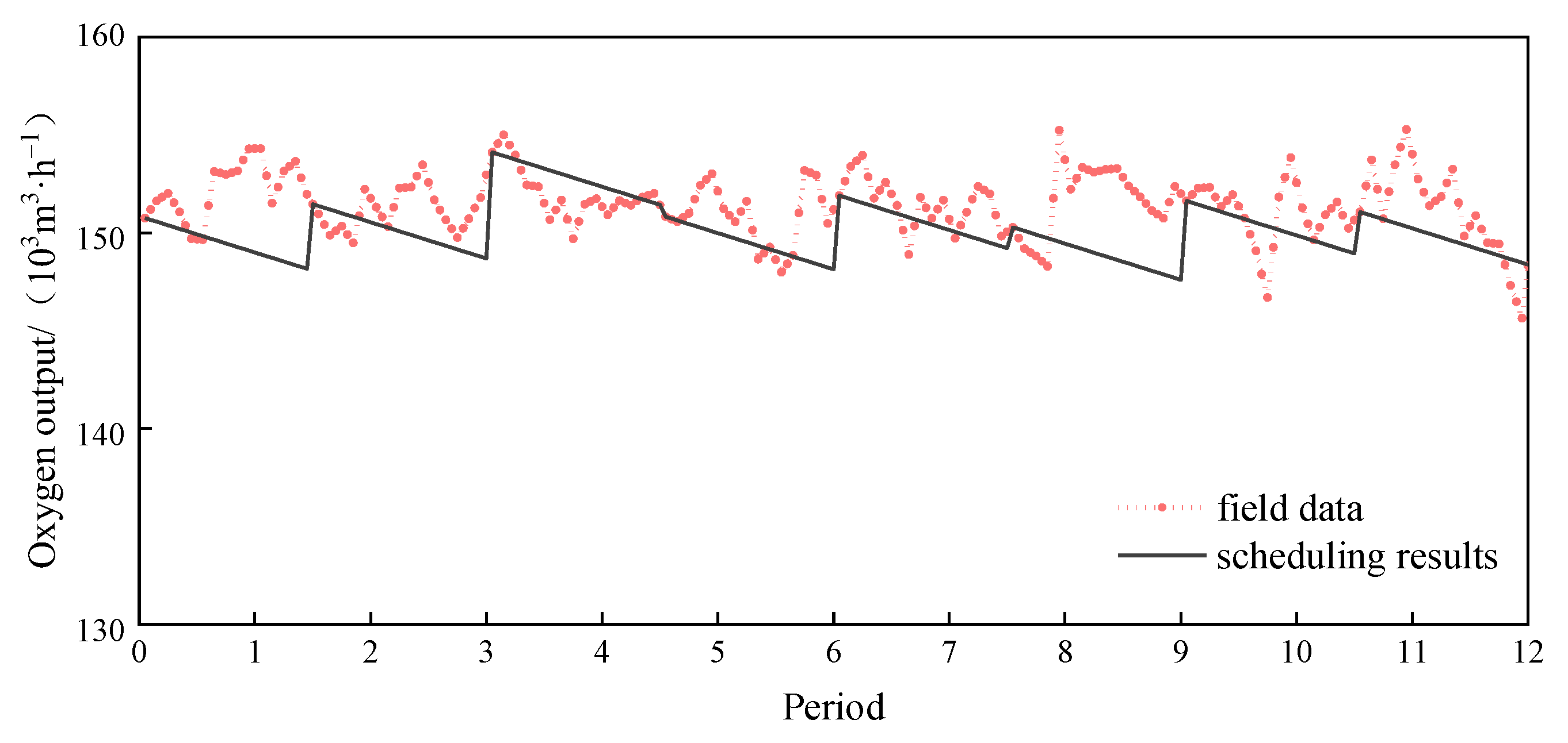
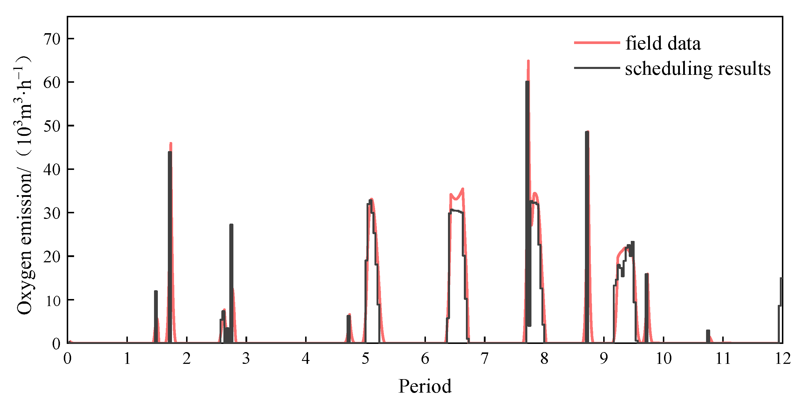
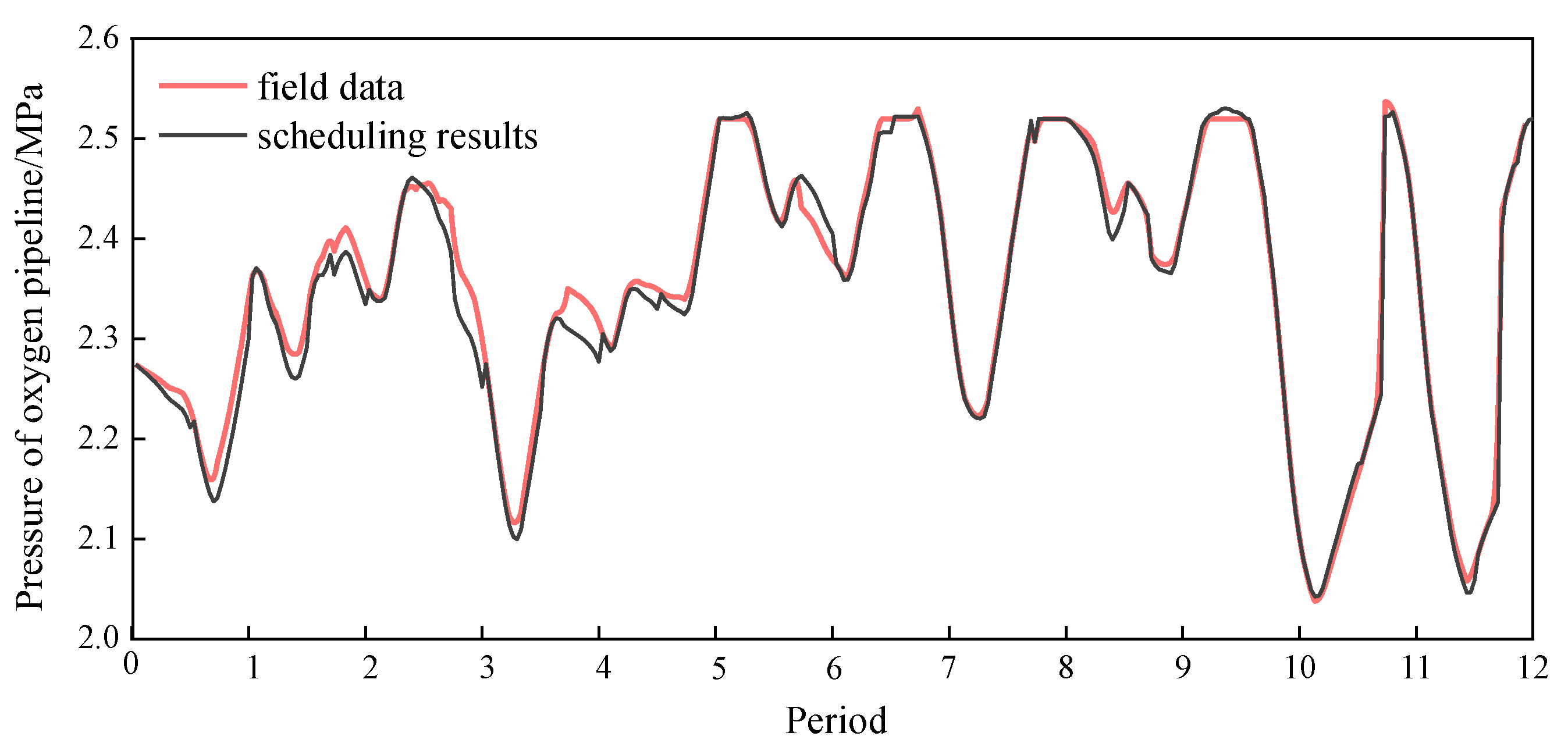
5.2. Analysis of the Scheduling Results of the Oxygen System

Substituting the forecast values of the GABP model in Section 5.1 as $D_t$ into the scheduling model, the scheduling of the oxygen system for a future period (15 data points, 30 min) could be realized. Through 12 independent scheduling calculations (12 periods), 12 sets of scheduling results were obtained, and the scheduling results are compared with the field data in Figure 6, Figure 7, Figure 8 and Figure 9.

As shown in Figure 6, the scheduling results of the oxygen output of the ASUs in each scheduling period declined, and the slope of the decline was the load change rate of the ASUs, which shows that under the current case conditions, oxygen was in a state of oversupply. The scheduling results of the oxygen output in Figure 6 are mostly lower than those of the field data. If on-site workers can perform load adjustments of the ASUs according to the scheduling results, the oxygen output can be reduced. By comparing the real data with the scheduling results in Figure 6, the oxygen output decrease rate at each time point could be calculated. To assess the situation over the entire period, a weighted average of all of the decrease rates was calculated, and the results indicate that the oxygen output of the ASUs after scheduling was approximately 1.38% lower than the field data on average.

Figure 7 compares the field data and scheduling results in terms of oxygen emissions, which shows that the oxygen emissions decreased after scheduling. By comparing the real data with the scheduling results in Figure 7, the oxygen emission decrease rate at each time point could be calculated. To assess the situation over the entire period, a weighted average of all of the decrease rates was calculated, and the results indicate that within the time frame of the case study, the oxygen emissions could be reduced by approximately 6.32% through scheduling on average.

Figure 8 shows a comparison between the scheduling results and the field data in terms of pipeline pressure. The calculation results show that, within the time range of the case study, the pipeline pressure after scheduling was approximately 0.61% lower than the field data.

The high-pressure oxygen in the pipeline has pressure energy, and the energy consumption required by the system is not only the energy consumption of oxygen separation (the oxygen separation energy consumption of ASUs is usually 0.4 kWh·m⁻³) but also the energy consumption of oxygen compression. The compression energy input by the system for the produced oxygen per unit of time is the compression power of oxygen, which is related to the pipeline pressure, as well as the oxygen output. For the convenience of comparison, the compression power can be quantified according to the energy consumption equation of multi-stage adiabatic compression, namely:

$$W_t=m\frac{n}{n-1}RT\left({\pi }^{\frac{n-1}{n}}-1\right)\delta \sum _{i=1}^{2}Ag{o}_{i,t}, \pi =\sqrt[m]{\frac{P_t}{P_0}}$$

(8)

where $W_t$ is the compression power of oxygen, m is the number of compression stages (in this paper, m = 3), n is the adiabatic coefficient, $\pi$ is the single-stage pressure ratio, $P_0$ is the ambient pressure, and $\delta$ is the conversion coefficient ($\delta$ = 0.0000124008).

According to the pressure shown in Figure 8, the calculated oxygen compression power is shown in Figure 9. Since the compression power is affected by both the oxygen output and the pipeline pressure, the scheduled compression power experienced a significant decrease compared to the unscheduled field data. The calculation results show that, within the time range of the case study, the energy consumption of the oxygen compression after the schedule decreased by approximately 1.60% compared to the field data.

Considering the loss of oxygen emissions, as well as the compression energy consumption, the total power consumption of the oxygen system after scheduling was reduced by approximately 1.38% compared to the field data. The total annual power consumption of the oxygen system of the case enterprise was approximately 120 million kWh, so approximately 16.42 million kWh/year of electricity can be saved through scheduling. Converted according to the electricity price of 0.55 RMB/kWh, optimal scheduling could bring economic benefits of 9.03 million RMB/year to the studied enterprise.

6. Conclusions

This study took a large-scale iron- and steel-making enterprise as a case study and developed a two-stage forecasting and scheduling model for reducing the energy consumption of its oxygen system. The GABP model was developed for oxygen demand forecasting, which is driven only by historical data. Additionally, an oxygen production scheduling model was developed for load-variable ASUs with an internal compression process, and the oxygen emissions and pipeline pressure are included in the objective function. Based on the case study, the following conclusions were obtained:

(1)

For the forecast of oxygen demand, the prediction accuracy of the GABP model is better than that of the ARIMA model. The case analysis showed that the average MAPE values for the 12 sets of data of the ARIMA and GABP models were 23.8% and 20.2%, respectively.

(2)

By comparing the scheduling results and the field data, it was found that after scheduling, the amount of oxygen emissions decreased by 6.32%, the pipeline pressure decreased by 0.61%, and the energy consumption of oxygen compression decreased by 1.6%. Considering the loss of oxygen emissions and the compression energy consumption, the total power consumption of the oxygen system was reduced by 1.38%, which means an annual saving of approximately 9.03 million RMB in electricity costs.

References

1. Ren, L.; Zhou, S.; Peng, T.; Ou, X. A review of CO2 emissions reduction technologies and low-carbon development in the iron and steel industry focusing on China. Renew. Sustain. Energy Rev. 2021, 143, 110846. [Google Scholar] [CrossRef]
2. Li, Z.; Hanaoka, T. Plant-level mitigation strategies could enable carbon neutrality by 2060 and reduce non-CO2 emissions in China’s iron and steel sector. One Earth 2022, 5, 932–943. [Google Scholar] [CrossRef]
3. Zhang, P.; Wang, L. Optimal shut-down policy for air separation units in integrated steel enterprises during a blast furnace blow-down. Ind. Eng. Chem. Res. 2017, 56, 2140–2149. [Google Scholar] [CrossRef]
4. Xu, W.; Tang, L.; Pistikopoulos, E.N. Modeling and solution for steelmaking scheduling with batching decisions and energy con-straints. Comput. Chem. Eng. 2018, 116, 368–384. [Google Scholar] [CrossRef]
5. Zhang, J.; Wang, G. Energy saving technologies and productive efficiency in the Chinese iron and steel sector. Energy 2008, 33, 525–537. [Google Scholar] [CrossRef]
6. Zhang, K.; Zheng, Z.; Zhang, L.; Liu, Y.; Chen, S. Method for Dynamic Prediction of Oxygen Demand in Steelmaking Process Based on BOF Technology. Processes 2023, 11, 2404. [Google Scholar] [CrossRef]
7. Rout, B.K.; Brooks, G.; Akbar Rhamdhani, M.; Li, Z.; Schrama, F.N.; Overbosch, A. Dynamic model of basic oxygen steelmaking process based on multizone reaction kinetics: Modeling of decarburization. Metall. Mater. Trans. B 2018, 49, 1022–1033. [Google Scholar] [CrossRef]
8. Xu, G.; Li, M.; Xu, J.W.; Jia, C.H.; Chen, Z.F. Control technology of end-point carbon in converter steelmaking based on func-tional digital twin model. J. Eng. 2019, 41, 521–527. (In Chinese) [Google Scholar]
9. Zhang, B.; Xue, Z.L.; Liu, K.; Bin Xiao, W. Development and application of prediction model for end-point manganese content in converter based on data from sub-lance. Adv. Mater. Res. 2013, 683, 497–503. [Google Scholar] [CrossRef]
10. Ruuska, J.; Sorsa, A.; Lilja, J.; Kauko, L. Mass-balance based multivariate modelling of basic oxygen furnace used in steel in-dustry. IFAC 2017, 50, 13784–13789. [Google Scholar]
11. Daniela, D.; Christopher, S.; Neslihan, D. Dynamic modeling and simulation of basic oxygen furnace (BOF) operation. Processes 2020, 8, 483–505. [Google Scholar]
12. Peng, S.-Y.; Zhang, G.-Y.; Li, H.-M. A novel modeling method based on support vector domain description and LS-SVM for steel-making process. In Proceedings of the 2008 International Conference on Machine Learning and Cybernetics, Kunming, China, 12–15 July 2008. [Google Scholar]
13. Jiang, S.; Shen, X.; Zheng, Z. Gaussian process-based hybrid model for predicting oxygen consumption in the converter steelmaking process. Processes 2019, 7, 352. [Google Scholar] [CrossRef]
14. Zhou, P.; Xu, Z.; Peng, X.; Zhao, J.; Shao, Z. Long-term prediction enhancement based on multi-output Gaussian process regression integrated with production plans for oxygen supply network. Comput. Chem. Eng. 2022, 163, 107844. [Google Scholar] [CrossRef]
15. Han, Z.; Zhao, J.; Wang, W. An optimized oxygen system scheduling with electricity cost consideration in steel industry. IEEE/CAA J. Autom. Sin. 2017, 4, 216–222. [Google Scholar] [CrossRef]
16. Zhang, P.; Wang, L.; Tong, L. MILP-based optimization of oxygen distribution system in integrated steel mills. Comput. Chem. Eng. 2016, 93, 175–184. [Google Scholar] [CrossRef]
17. Xu, Z.; Zheng, Z.; Gao, X.; Shen, X. Reducing the fluctuation of oxygen demand in a steel plant through optimal production scheduling. J. Clean. Prod. 2020, 282, 124529. [Google Scholar] [CrossRef]
18. Zhang, L.; Zheng, Z.; Xu, Z.; Chai, Y. Optimal scheduling of oxygen system in steel enterprises considering uncertain demand by decreasing pipeline network pressure fluctuation. Comput. Chem. Eng. 2022, 160, 107692. [Google Scholar] [CrossRef]
19. Zhang, L.; Zheng, Z.; Chai, Y.; Xu, Z.; Zhang, K.; Liu, Y.; Chen, S.; Zhao, L. ASU model with multiple adjustment types for oxygen scheduling concerning pipe pressure safety in steel enterprises. Appl. Energy 2023, 343, 120986. [Google Scholar] [CrossRef]
20. Liu, C.; Tang, L.; Zhao, C. A novel dynamic operation optimization method based on multiobjective deep reinforcement learning for steelmaking process. In IEEE Transactions on Neural Networks and Learning System; IEEE: Piscataway, NJ, USA, 2023. [Google Scholar] [CrossRef]
21. Han, Z.; Zhao, J.; Wang, W.; Liu, Y. A two-stage method for predicting and scheduling energy in an oxygen/nitrogen system of the steel industry. Control Eng. Pract. 2016, 52, 35–45. [Google Scholar] [CrossRef]
22. Jiang, .S.L.; Peng, G.; Bogle, I.D.L.; Zheng, Z. Two-stage robust optimization approach for flexible oxygen distribution under uncertainty in integrated iron and steel plants. Appl. Energy 2022, 306, 118022. [Google Scholar] [CrossRef]
23. Zhang, L.; Zhang, K.; Zheng, Z.; Chai, Y.; Lian, X.; Zhang, K.; Xu, Z.; Chen, S. Two-stage distributionally robust integrated scheduling of oxygen distribution and steelmaking-continuous casting in steel enterprises. Appl. Energy 2023, 351, 121788. [Google Scholar] [CrossRef]
24. Box, G.E.P.; Jenkins, G.M.; Reinsel, G.C.; Ljung, G.M. Time Series Analysis: Forecasting and Control; John Wiley & Sons: Hoboken, NJ, USA, 2015. [Google Scholar]
25. Ding, S.; Su, C.; Yu, J. An optimizing BP neural network algorithm based on genetic algorithm. Artif. Intell. Rev. 2011, 36, 153–162. [Google Scholar] [CrossRef]
26. Wang, F.; Su, H.; Jing, K. Dam safety monitoring model based on ARIMA-ANN. Eng. J. Wuhan Univ./Wuhan Daxue Xuebao 2010, 43, 585–588. [Google Scholar]
Figure 1. The oxygen system of a large-scale iron- and steel-making mill.
Applsci 13 11618 g001
Figure 2. Neural network topology.
Applsci 13 11618 g002
Figure 3. Oxygen demand: ARIMA model forecasting vs. field data.
Applsci 13 11618 g003
Figure 4. Oxygen demand: GABP model forecasting vs. field data.
Applsci 13 11618 g004
Figure 5. Forecasting error: ARIMA model vs. GABP model.
Applsci 13 11618 g005
Figure 6. Oxygen output of the ASUs: Scheduling results vs. field data.
Applsci 13 11618 g006
Figure 7. Emission loss of the oxygen system: Scheduling results vs. field data.
Applsci 13 11618 g007
Figure 8. Pressure of the oxygen pipeline: Scheduling results vs. field data.
Applsci 13 11618 g008
Figure 9. Compressor energy consumption of the oxygen system: Scheduling results vs. field data.
Applsci 13 11618 g009