
Analysis of Grinding Flow Field under Minimum Quantity Lubrication Condition

Abstract
:1. Introduction
2. Flow Field Analysis of the Grinding Wheel
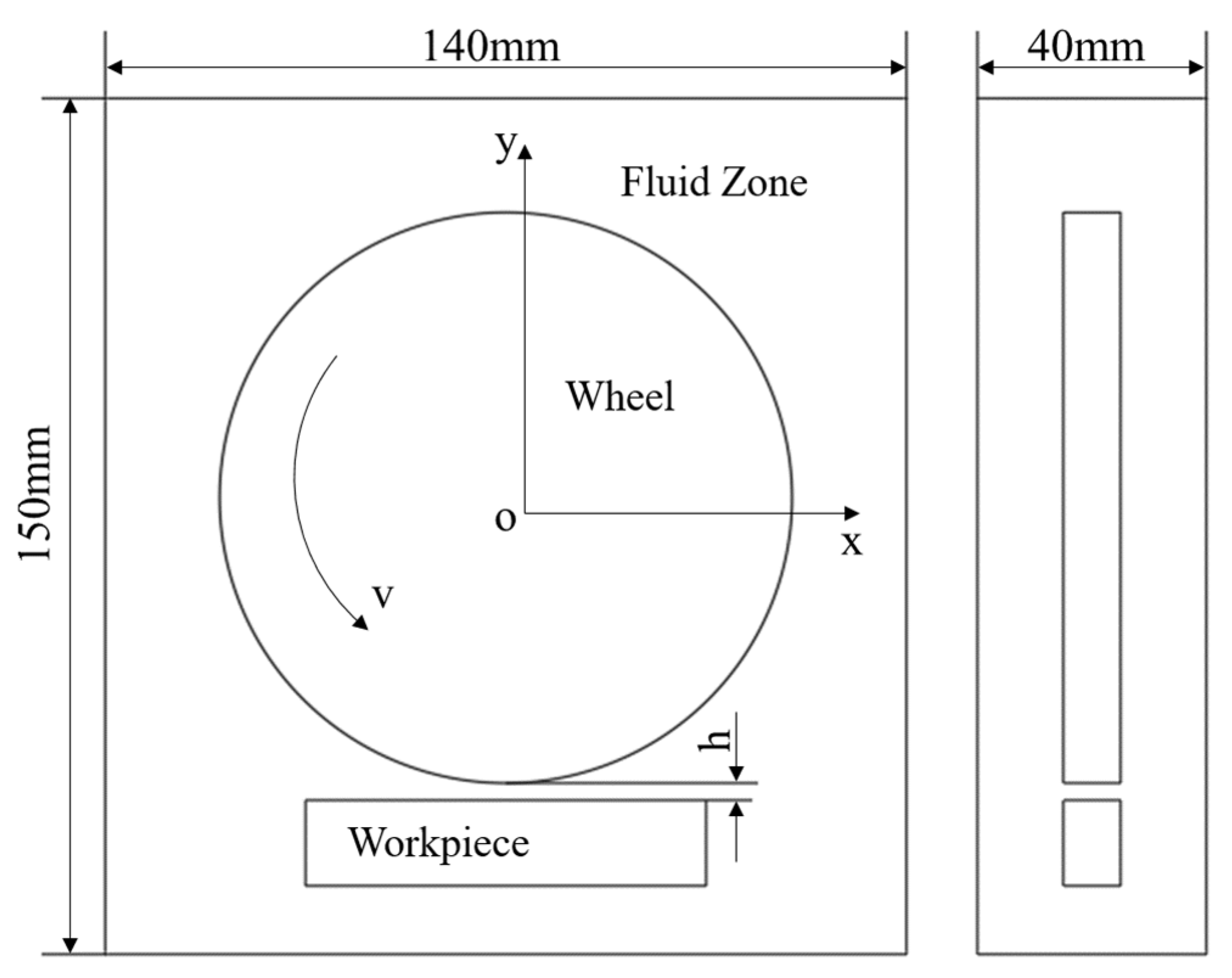
2.1. Theoretical Modeling of the Grinding Wheel Flow Field
2.2. Two-Phase Flow Model
3. Simulation and Analysis of Three-Dimensional Grinding Wheel Flow Field
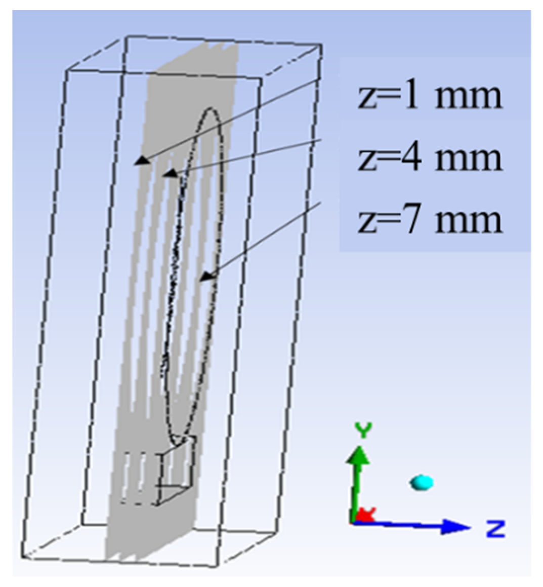
3.1. Three-Dimensional Simulation Model Construction and Parameter Setting
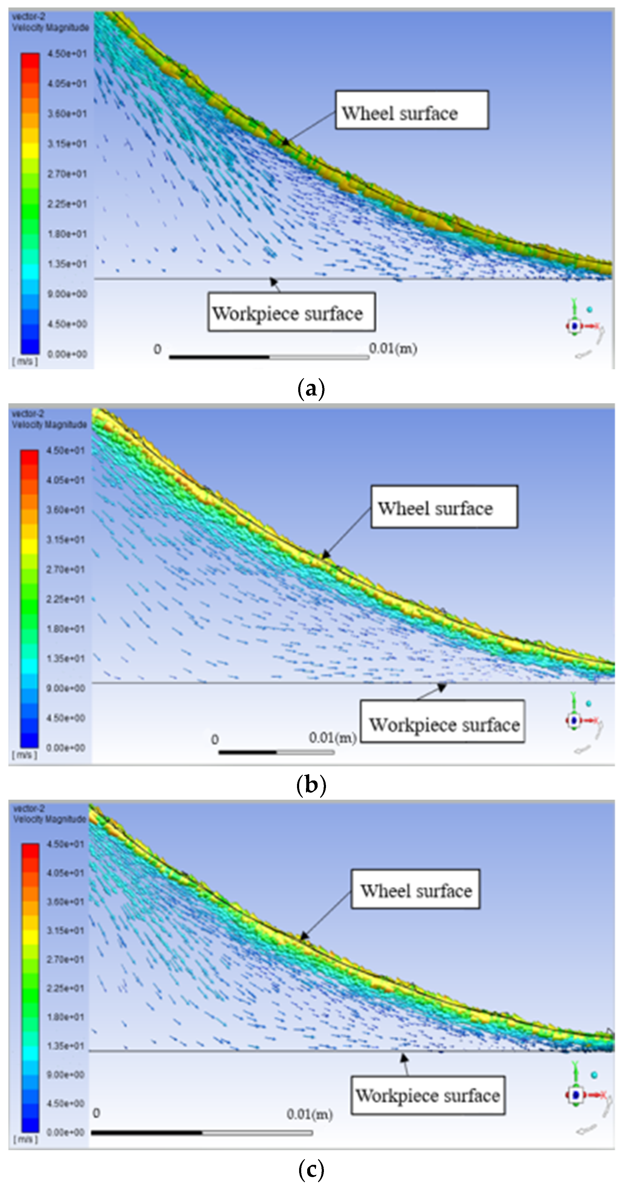
3.2. Characterization of Velocity Distribution of Flow Field
3.3. Simulation and Analysis of the Grinding Wheel Flow Field under MQL Conditions
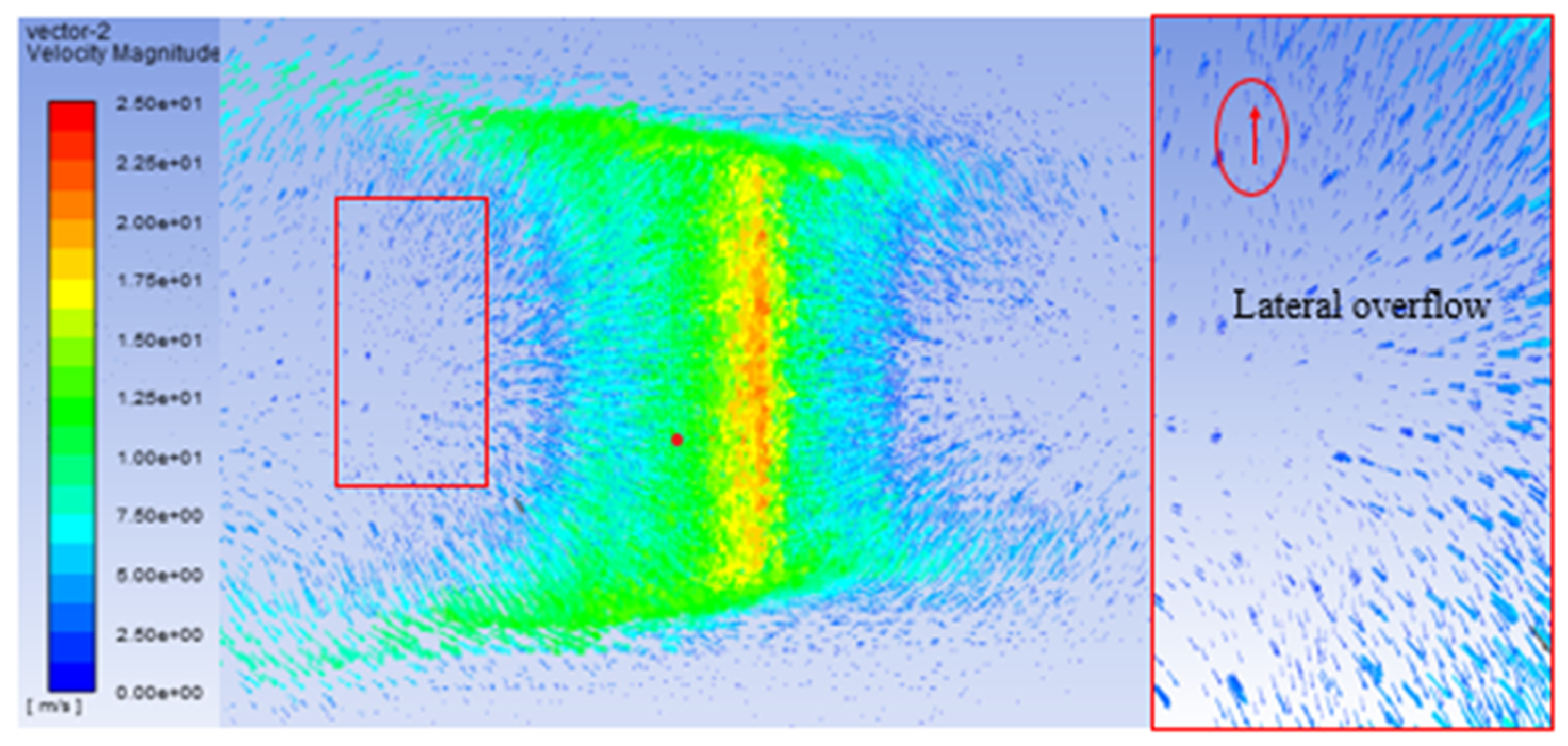
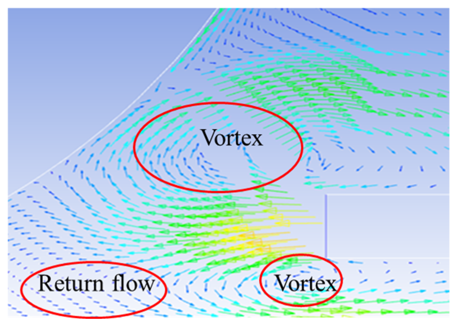
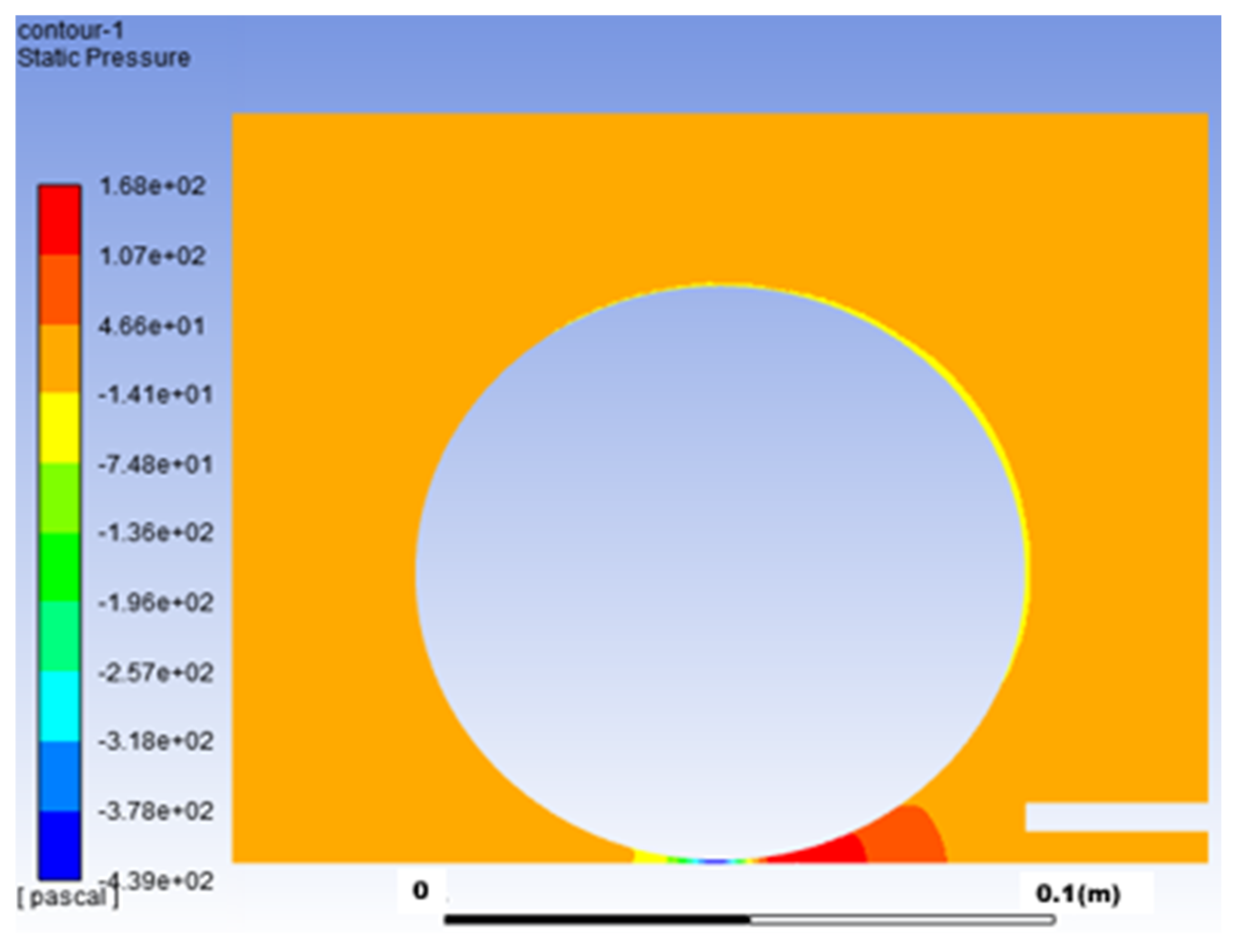
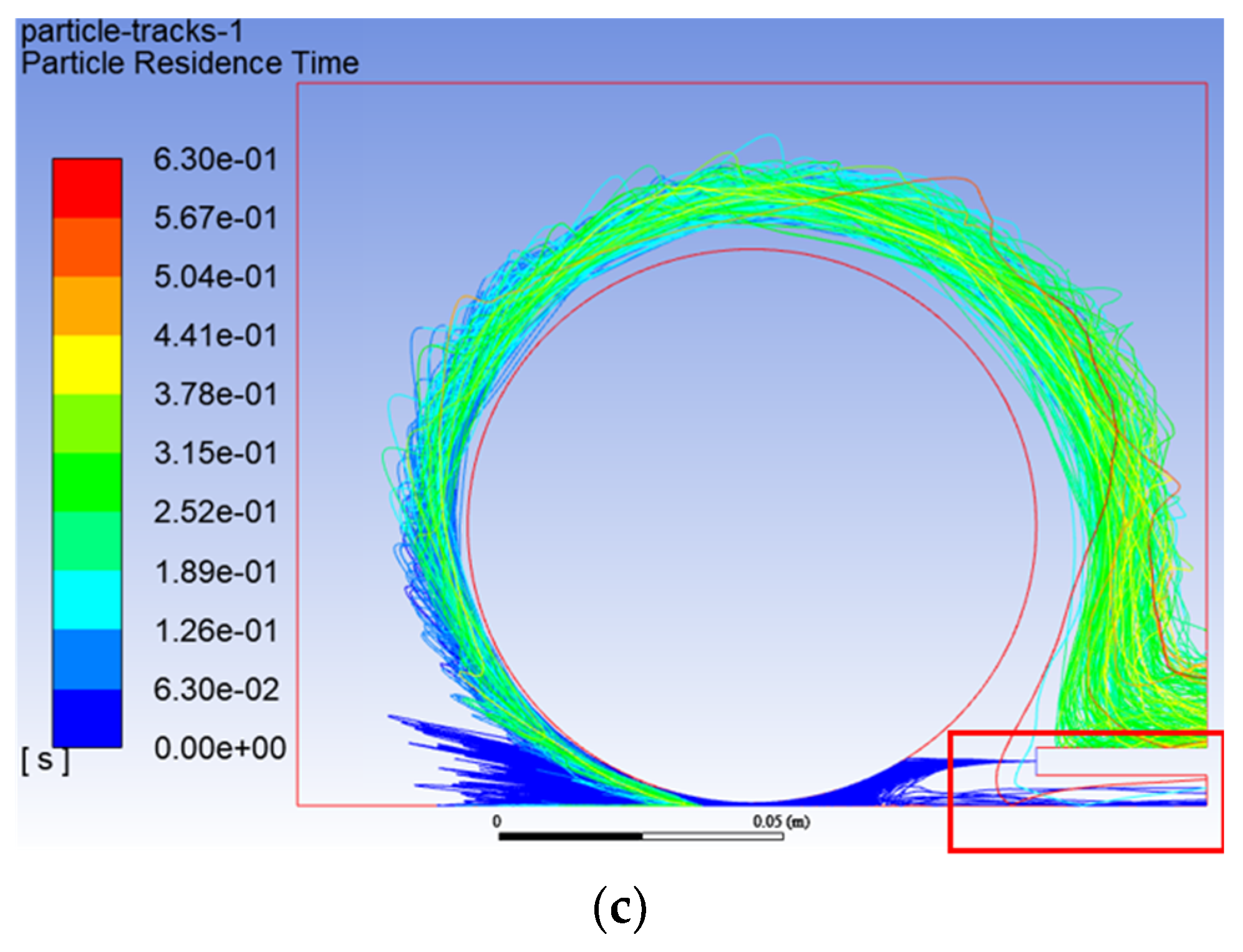
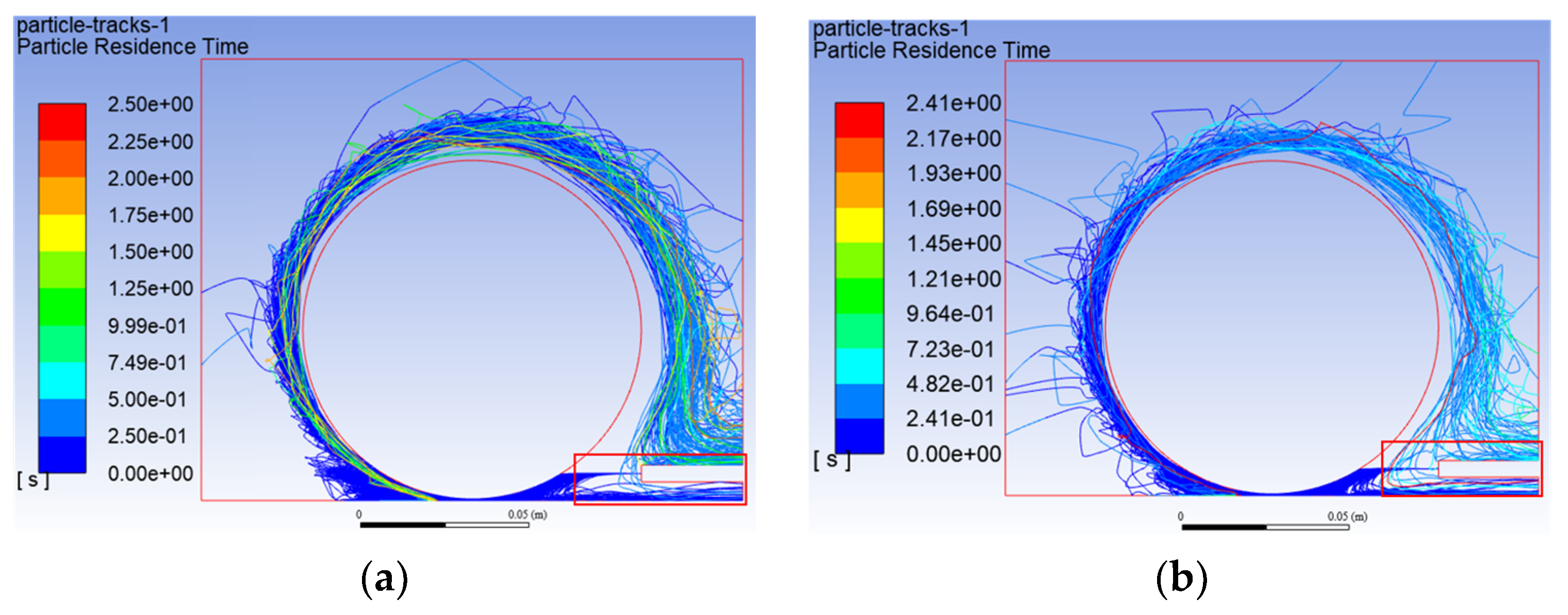
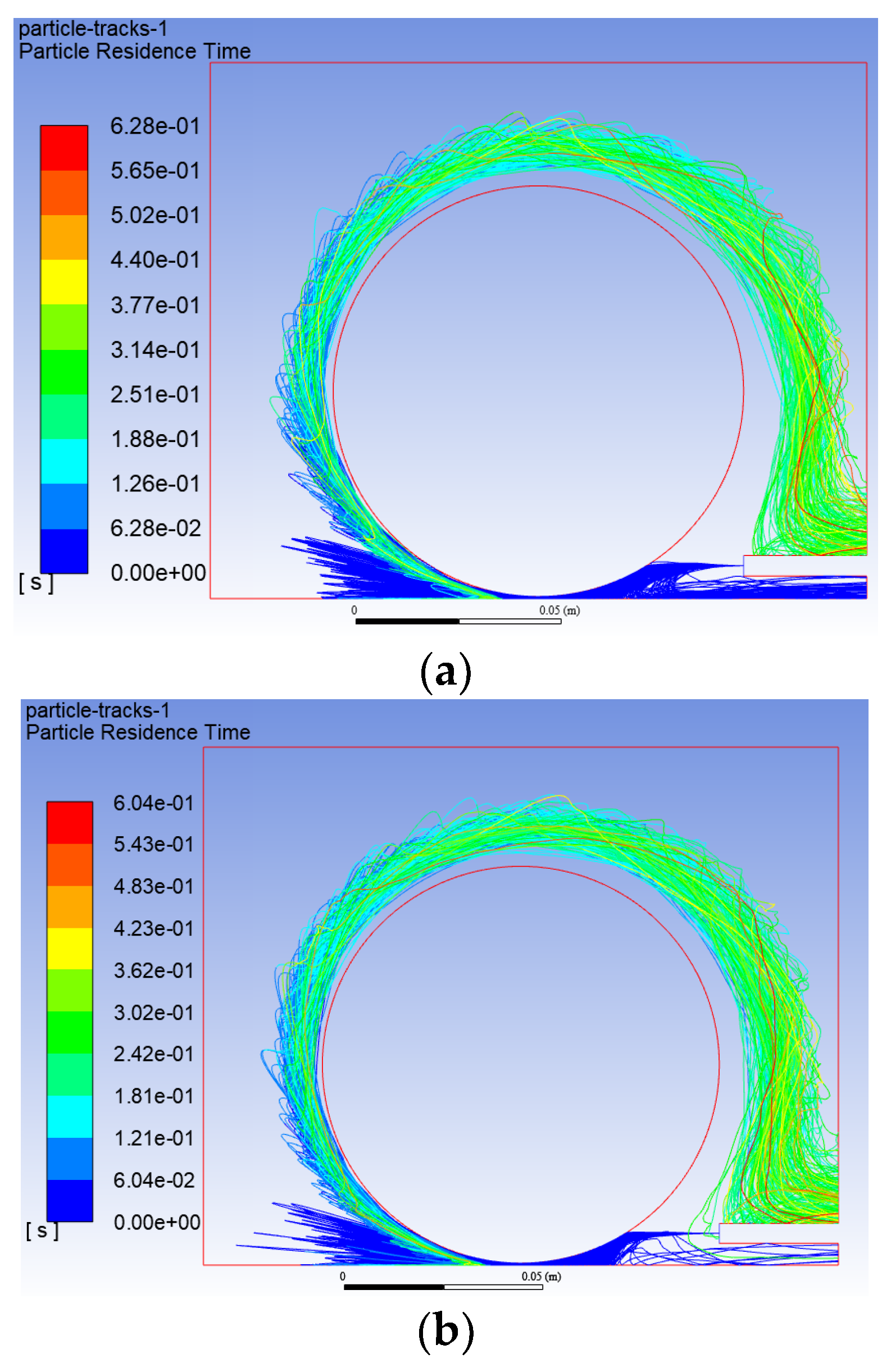
3.3.1. The Wedge Region under the Influence of MQL Jet
3.3.2. Effect of MQL Jet on the Flow Field of the Grinding Wheel
- Effect of Grinding Fluid Flow on Effective Flow Rate
- 2.
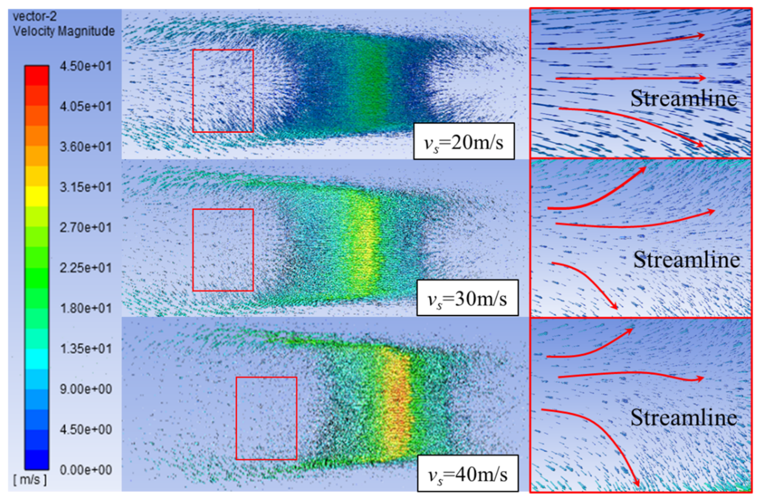
- Effect of the grinding wheel linear velocity on effective flow rate
- 3.
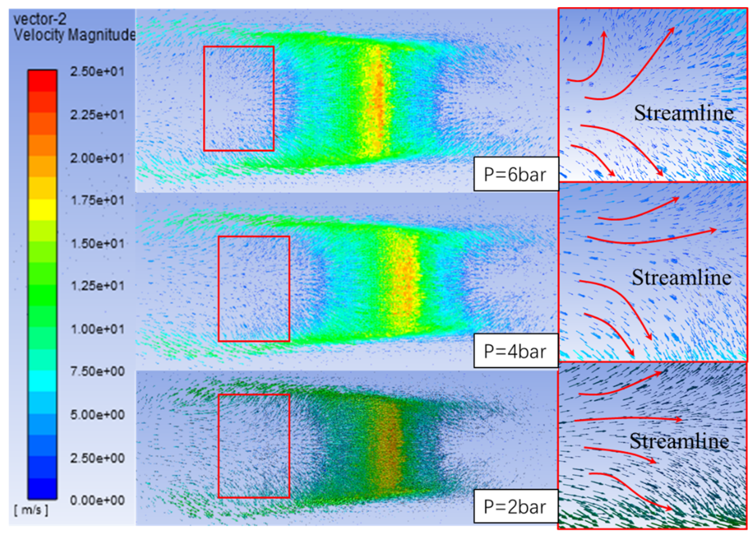
- Effect of the compressed gas pressure on effective flow rate of the grinding fluid
4. Experimental Verification
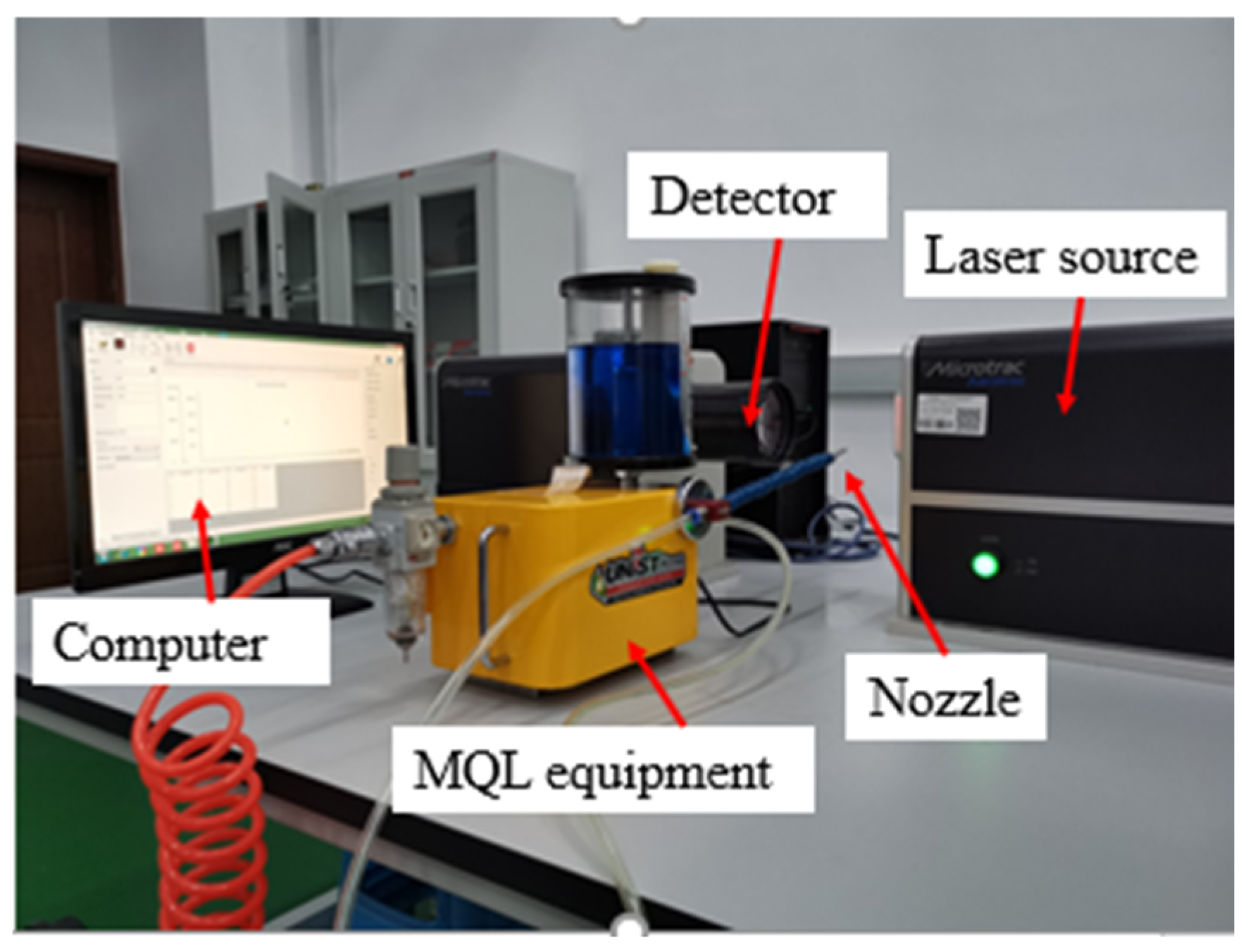
4.1. Test the Droplet Size
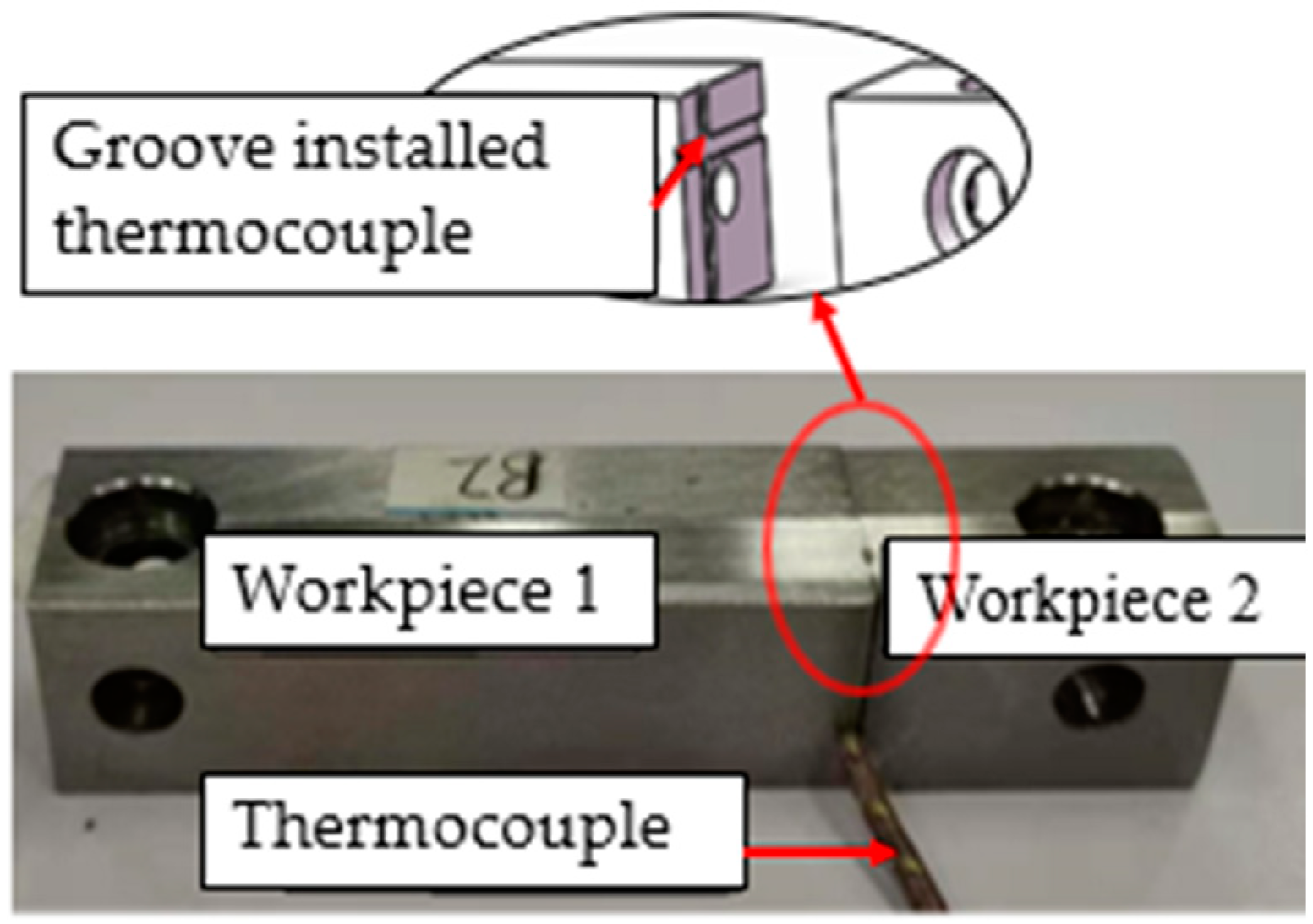
4.2. Grinding Temperature Measurement
4.3. Discussion
5. Conclusions
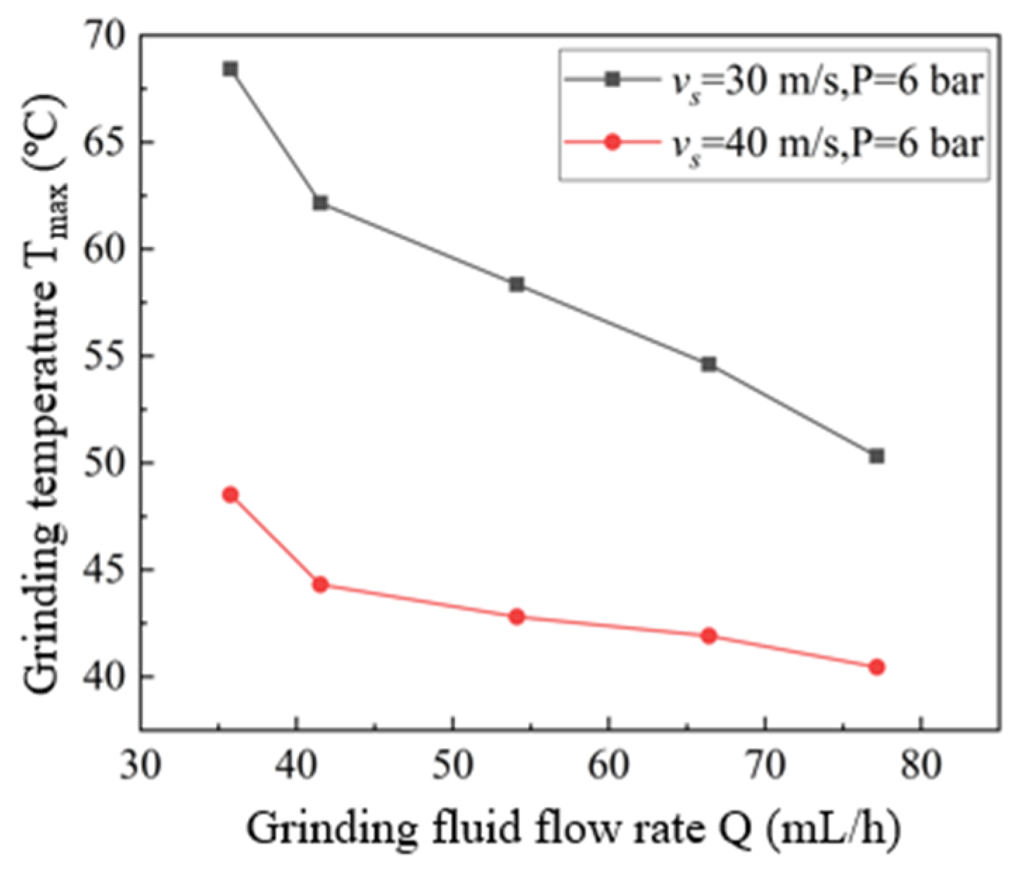
- (1)
- There is a clear relationship between the grinding temperature and the grinding fluid flow rate. The grinding temperature decreases as the grinding fluid flow rate increases. When the flow rate of the grinding fluid is lower than 45 mL/h, the grinding temperature is inclined to reduce more with the increase in the flow rate of the grinding fluid. When the flow rate of the grinding fluid is larger than 45 mL/h, the tendency of grinding temperature decreasing with the increase in grinding fluid flow rate slows down.
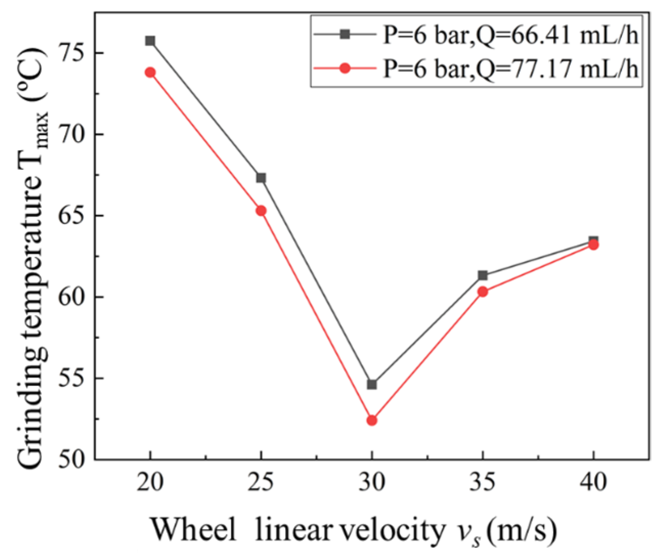
- (2)
- The change in speed of the grinding wheel affects the flow rate of the grinding fluid, which in turn affects the grinding temperature. As the linear speed of the grinding wheel improves, the effective flow rate of the grinding fluid first improves and then reduces. Accordingly, the grinding temperature first reduces and then improves. When the linear speed is less than 30 m/s, with the increase in linear speed, the effective flow rate increases and the grinding temperature decreases. When the linear speed is greater than 30 m/s, with the increase in linear speed, the effective flow of grinding fluid decreases and the grinding temperature increases.
- (3)
- The compressed gas pressure affects the effective flow rate of grinding fluid and the grinding temperature. As the compressed gas pressure increases, the effective flow rate of grinding fluid grows first and then reduces. Accordingly, the grinding temperature decreases first and then increases. The temperature curve inflection point is different for different grinding wheel linear speed.
Author Contributions
Funding
Institutional Review Board Statement
Informed Consent Statement
Data Availability Statement
Conflicts of Interest
References
- Li, K.; Chou, S. Experimental evaluation of minimum quantity lubrication in near micro-milling. J. Mater. Process. Tech. 2010, 210, 2163–2170. [Google Scholar] [CrossRef]
- Sun, C.; Xiu, S.; Hong, Y.; Kong, X.; Lu, Y. Prediction on residual stress with mechanical-thermal and transformation coupled in DGH. Int. J. Mech. Sci. 2021, 179, 105629. [Google Scholar] [CrossRef]
- Zhang, Y.; Wang, Q.; Li, C.; Piao, Y.; Hou, N.; Hu, K. Characterization of surface and subsurface defects induced by abrasive machining of optical crystals using grazing incidence X-ray diffraction and molecular dynamics. J. Adv. Res. 2021, 36, 51–66. [Google Scholar] [CrossRef]
- Ding, Z.; Sun, G.; Guo, M.; Jiang, X.; Li, B.; Liang, S. Effect of phase transition on micro-grinding-induced residual stress. J. Mater. Process. Tech. 2020, 281, 116647. [Google Scholar] [CrossRef]
- Ji, X.; Li, B.; Zhang, X.; Liang, S. The effects of minimum quantity lubrication (MQL) on machining force, temperature, and residual stress. Int. J. Precis. Eng. Manuf. 2014, 15, 2443–2451. [Google Scholar] [CrossRef]
- Shao, Y.; Fergani, O.; Ding, Z.; Li, B.; Liang, S. Experimental investigation of residual stress in minimum quantity lubrication grinding of AISI 1018 steel. J. Manuf. Sci. Eng. 2016, 138, 711–718. [Google Scholar] [CrossRef]
- Zhuang, K.; Fu, C.; Weng, J.; Hu, C. Cutting edge microgeometries in metal cutting: A review. Int. J. Adv. Manuf. Tech. 2021, 116, 2045–2092. [Google Scholar] [CrossRef]
- Liao, Y.; Liao, C.; Lin, H. Study of oil water ratio and flow rate of MQL fluid in high speed milling of Inconel 718. Int. J. Precis. Eng. Manuf. 2017, 18, 257–262. [Google Scholar] [CrossRef]
- Huang, X.; Ren, Y.; Li, T.; Zhou, Z.; Zhang, G. Influence of minimum quantity lubrication parameters on grind-hardening process. Mater. Manuf. Process. 2018, 33, 69–76. [Google Scholar] [CrossRef]
- Balan, A.; Kullarwar, T.; Vijayaraghavan, L.; Krishnamurthy, R. Computational fluid dynamics analysis of MQL spray parameters and its influence on superalloy grinding. Mach. Sci. Technol. 2017, 21, 603–616. [Google Scholar] [CrossRef]
- Silva, L.; Correa, E.; Brandao, J.; De Avila, R. Environmentally friendly manufacturing: Behavior analysis of minimum quantity of lubricant—MQL in grinding process. J. Clean. Prod. 2020, 256, S0959652613000383. [Google Scholar] [CrossRef]
- Tawakoli, T.; Hadad, M.; Sadeghi, M. Influence of Oil Mist Parameters on Minimum Quantity Lubrication—MQL Grinding Process. Int. J. Mach. Tools Manuf. 2010, 50, 521–531. [Google Scholar] [CrossRef]
- Liu, H.; Song, W.; Niu, Y.; Zio, E. Generalized cauchy method for remaining useful life prediction of wind turbine gearboxes. Mech. Syst. Signal. 2021, 153, 107471. [Google Scholar] [CrossRef]
- Morgan, M.; Jackson, A.; Wu, H. Optimisation of fluid application in grinding. Cirp Aann-Manuf. Techn. 2008, 57, 363–366. [Google Scholar] [CrossRef]
- Ebbrell, S.; Woolley, N.; Tridimas, Y.; Allanson, D.; Rowe, W. The effects of cutting fluid application methods on the grinding process. Int. J. Mach. Tool. Manuf. 2000, 40, 209–223. [Google Scholar] [CrossRef]
- Zhang, Y.; Li, C.; Jia, D.; Zhang, D.; Zhang, X. Experimental evaluation of MoS2 nanoparticles in jet MQL grinding with different types of vegetable oil as base oil. J. Clean. Prod. 2015, 87, 930–940. [Google Scholar] [CrossRef]
- Hadad, M.; Sadeghi, B. Thermal analysis of minimum quantity lubrication-MQL grinding process. Int. J. Mach. Tool. Manuf. 2012, 63, 1–15. [Google Scholar] [CrossRef]
- Baumgart, C.; Radziwill, J.; Kuster, F. A study of the interaction between coolant jet nozzle flow and the airflow around a grinding wheel in cylindrical grinding. Procedia CIRP 2017, 58, 517–522. [Google Scholar] [CrossRef]
- Mandal, B.; Singh, R.; Das, S.; Banerjee, S. Improving grinding performance by controlling air flow around a grinding wheel. Int. J. Mach. Tool. Manuf. 2011, 51, 670–676. [Google Scholar] [CrossRef]
- Li, C.; Cai, G.; Xiu, S.; Li, Q. Material removal model and experimental verification for abrasive jet precision finishing with wheel as restraint. Key Eng. Mater. 2006, 304–305, 555–559. [Google Scholar] [CrossRef]
- Cengel, Y.A.; Cimbala, J.M. Fluent Mechanics: Fundamentals and Applications, 4th ed.; McGraw-Hill Education (Asia): Singapore, 2013; pp. 138–154. [Google Scholar]
- Zhu, D.; Feng, X.; Xu, X.; Yang, Z.; Li, W.; Yan, S. Robotic grinding of complex components: A step towards efficient and intelligent machining-challenges, solutions, and applications. Robot. Cim-Integr. Manuf. 2020, 65, 101908. [Google Scholar] [CrossRef]
- Jia, D.; Li, C.; Zhang, D.; Zhang, Y.; Zhang, X. Experimental verification of nano-particle jet minimum quantity lubrication effectiveness in grinding. J. Nanopart. Res. 2015, 16, 2758. [Google Scholar] [CrossRef]


| Items | Settings |
|---|---|
| Solvers | 3D Segregated pressure-based |
| Turbulence model | Renormalization Group k-epsilon Model |
| Wall | No slip, standard wall function |
| Moving Wall | vs = 20, 30, 40 m/s |
| Operating pressure | Atmospheric pressure |
| Pressure outlet boundaries | P = 0 Pa |
| Minimum clearance | h = 0.05, 0.1, 1 mm |
| Items | Values | DPM Type |
|---|---|---|
| Wheel diameter | 100 mm | |
| Wheel linear velocity | 40 m/s | |
| Minimum gap | 0.05 mm | |
| pressure outlet boundary | 0 Bar | |
| pressure inlet boundary | 2, 4, 6 Bar | Escape |
| Workpiece wall | Fixed wall | Reflect |
| Wheel wall | Rotating wall | Reflect |
| Nozzle wall | Fixed wall | Reflect |
| Fluid Materials | Standard air | |
| Environmental temperature | 25 °C | |
| Flow rate of grinding fluid | 54.11, 66.41, 77.17 mL/h |
| Wheel Rotation Velocity νs (m/s) | 20, 25, 30, 35, 40 |
|---|---|
| Feed speed vw (m/s) | 0.01 |
| Cutting depth αe (μm) | 8 |
| MQL flow rate Q (mL/h) | 35.77, 41.53, 54.11, 66.41, 77.17 |
| Compressed P (bar) | 2, 3, 4, 5, 6 |
Disclaimer/Publisher’s Note: The statements, opinions and data contained in all publications are solely those of the individual author(s) and contributor(s) and not of MDPI and/or the editor(s). MDPI and/or the editor(s) disclaim responsibility for any injury to people or property resulting from any ideas, methods, instructions or products referred to in the content. |
© 2023 by the authors. Licensee MDPI, Basel, Switzerland. This article is an open access article distributed under the terms and conditions of the Creative Commons Attribution (CC BY) license (https://creativecommons.org/licenses/by/4.0/).
Share and Cite
Ni, W.; Ding, Z.; Sun, J. Analysis of Grinding Flow Field under Minimum Quantity Lubrication Condition. Appl. Sci. 2023, 13, 11664. https://doi.org/10.3390/app132111664
Ni W, Ding Z, Sun J. Analysis of Grinding Flow Field under Minimum Quantity Lubrication Condition. Applied Sciences. 2023; 13(21):11664. https://doi.org/10.3390/app132111664
Chicago/Turabian StyleNi, Weihua, Zishan Ding, and Jian Sun. 2023. "Analysis of Grinding Flow Field under Minimum Quantity Lubrication Condition" Applied Sciences 13, no. 21: 11664. https://doi.org/10.3390/app132111664
APA StyleNi, W., Ding, Z., & Sun, J. (2023). Analysis of Grinding Flow Field under Minimum Quantity Lubrication Condition. Applied Sciences, 13(21), 11664. https://doi.org/10.3390/app132111664