Two-Stage Fusion-Based Audiovisual Remote Sensing Scene Classification

Abstract

Scene classification in remote sensing is a pivotal research area, traditionally relying on visual information from aerial images for labeling. The introduction of ground environment audio as a novel geospatial data source adds valuable information for scene classification. However, bridging the structural gap between aerial images and ground environment audio is challenging, rendering popular two-branch networks ineffective for direct data fusion. To address this issue, the study in this research presents the Two-stage Fusion-based Audiovisual Classification Network (TFAVCNet). TFAVCNet leverages both audio and visual modules to extract deep semantic features from ground environmental audio and remote sensing images, respectively. The audiovisual fusion module combines and fuses information from both modalities at the feature and decision levels, facilitating joint training and yielding a more-robust solution. The proposed method outperforms existing approaches, as demonstrated by the experimental results on the ADVANCE dataset for remote sensing audiovisual scene classification, offering an innovative approach to enhanced scene classification.

1. Introduction

Remote sensing offers a variety of data sources for surface feature recognition and classification, enhancing our understanding of the Earth’s surface [1,2]. Due to the advancement of remote sensing satellites and various social media, traditional remote sensing scene classification tasks are typically based on images, using passive or active sensors [3,4,5,6] and various street view images. In recent years, urban planning [7], environmental monitoring [8,9], and various other fields have greatly benefited from the extensive acquisition of remote sensing data and the rapid advancements in remote sensing technology. On the other hand, as a result of the ongoing development of sound recording software and the rising demand for various acoustic tasks, scene classification tasks based on audio have advanced significantly [10,11,12], such as speech command recognition [13], emotion recognition [14], and audio event classification [15,16]. When classifying an acoustic scene, the input is often a brief audio recording; however, when classifying a visual scene, the input can be either an image or a brief video clip.

Advanced audio scene-classification algorithms currently in use are typically based on spectral features, most frequently log-Mel spectrograms, and convolutional neural network structures, as CNN structures aid in providing general classification information for longer segments of acoustic scenes [17]. The conventional CNN architecture may execute downsampling operations on the time dimension and feature dimension while continually learning acoustic information using several convolutional layers and pooling layers. Based on this, Ren et al. [18] proposed a dilated convolutional kernel that allows achieving a comparable receptive field without intermediate pooling to improve the performance of the acoustic scene classification system in the context of local feature acquisition. In the following study, Koutine et al. [19] confirmed that restricting the size of the receptive field can effectively improve the performance of acoustic scene classification. Researchers have extended the commonly used CNN structure in anticipation of improving the learning ability of acoustic features. Basbug and Sert [20] drew inspiration from the field of computer vision, adopted a spatial pyramid pooling strategy, pooled and combined features at different spatial resolutions, and further improved the performance of acoustic feature extraction. The attention mechanism was also used to build an audio scene classification system in addition to the CNN structure and its variations for acoustic scene classification. An attention mechanism allows the neural network to concentrate on a particular subset of input data because different time segments of ambient audio recordings have varying impacts on the categorization of acoustic scenes. Li et al. [21] introduced a multi-level attention model in the network’s feature-learning section to improve feature-learning performance. At the same time, the attention mechanism can also be applied to the pooling operation of the feature map. Wang et al. [22] used Self-Determination CNNs (SD-CNNs) to identify the acoustic events due to overlapping higher uncertainty frame information.

In contrast, remote sensing image classification methods have a longer history and a greater variety of methodologies, which are either based on the traditional handcrafted features or the deep learning ones. Early scene classification mainly depended on manually created features. There are numerous traditional techniques for extracting hand-crafted features, including the Histogram of Oriented Gradients (HOG) [23], texture descriptors [24], GIST [25], color histograms [26], and Scale-Invariant Feature Transform (SIFT) [27]. Deep learning methods have also been introduced into the field of remote sensing. Cheng et al. [28] first used Convolutional Neural Networks (CNN) for scene classification of high-resolution remote sensing images. Zhou et al. [29] introduced deep learning to process high-resolution remote sensing images, proposed a method for automatically learning feature representation, and experimentally demonstrated its effectiveness in scene classification tasks. Inspired by the mechanism of attention, Wang et al. [5] introduced a recurrent attention mechanism combined with deep learning methods to solve the scene classification problem of high-resolution remote sensing images, providing a new method for image processing and classification in the field of remote sensing. Vision Transformer (ViT) has recently been used for scene classification and has shown good results. For image classification tasks, the Vision Transformer (ViT) model uses attention-based deep learning. The ViT model uses a self-attention mechanism to capture the global information in the image, in contrast to the conventional Convolutional Neural Network (CNN), which views the image as a collection of segmented blocks. At the moment, researchers are attempting to use Transformers for remote sensing tasks. For example, Guo et al. [30] proposed a Transformer method based on channel–spatial attention for remote sensing image scene classification; Xu et al. [31] proposed an efficient multi-scale Transformer named EMTCAL and a cross-level attentional learning method for remote sensing scene classification; Li et al. [32] proposed a method called Reformer for remote sensing scene classification. This method aims to improve the accuracy and effectiveness of remote sensing image scene classification by combining a residual network and Transformer.

However, whether applied to audio scene classification or remote sensing image classification, prevailing methodologies predominantly rely on data from a singular modality. In practical, real-world scenarios, human perception and comprehension of natural environments inherently involve the integration of multiple sensory modalities, particularly sight and hearing. Human perceptual research underscores the inherent complementarity of sound and visual information in the comprehensive understanding of environmental scenes [33]. For example, within an airport setting, aerial images captured from the air by aircraft provide an expansive, bird’s-eye view of the airport’s layout. At the same time, people can hear some ground environment sounds including human conversations, airport announcements, and unique engine sounds on the ground. In light of the foregoing analysis grounded in common sense, it is reasonable to explore the amalgamation of sound and visual information for the purpose of scene classification. Researchers are increasingly interested in multimodal data fusion due to the continuous evolution of remote sensing and sensor instrumentation. Emerging as a valuable sensory data source, ground environment audio data can contribute significantly to the classification of surface scenes by furnishing information on environmental acoustics, such as wildlife vocalizations and traffic sounds. This auditory information can help classify various scenes. Hence, researchers have initiated the exploration of sound–image fusion for multimodal remote sensing scene classification, striving to enhance classification precision and robustness [34]. Saurabh et al. [35] proposed a method of integrating local context information into a self-attention model to improve scene classification, using local and global temporal relationships between video frames to obtain a more-comprehensive contextual representation of a single frame. In addition to relying on the attention mechanism to improve the accuracy of multi-modal scene classification, technical improvement on the feature extraction level is another research hotspot. Kurcius et al. [36] combined the latest method of audiovisual feature extraction with the multi-resolution feature bag model to improve the feature extraction technology and proposed a unique audiovisual environment perception model based on compressed sensing theory [37] to improve the environment scene classification performance. As research endeavors in image and audio scene classification tasks advance, this interdisciplinary approach holds substantial promise.

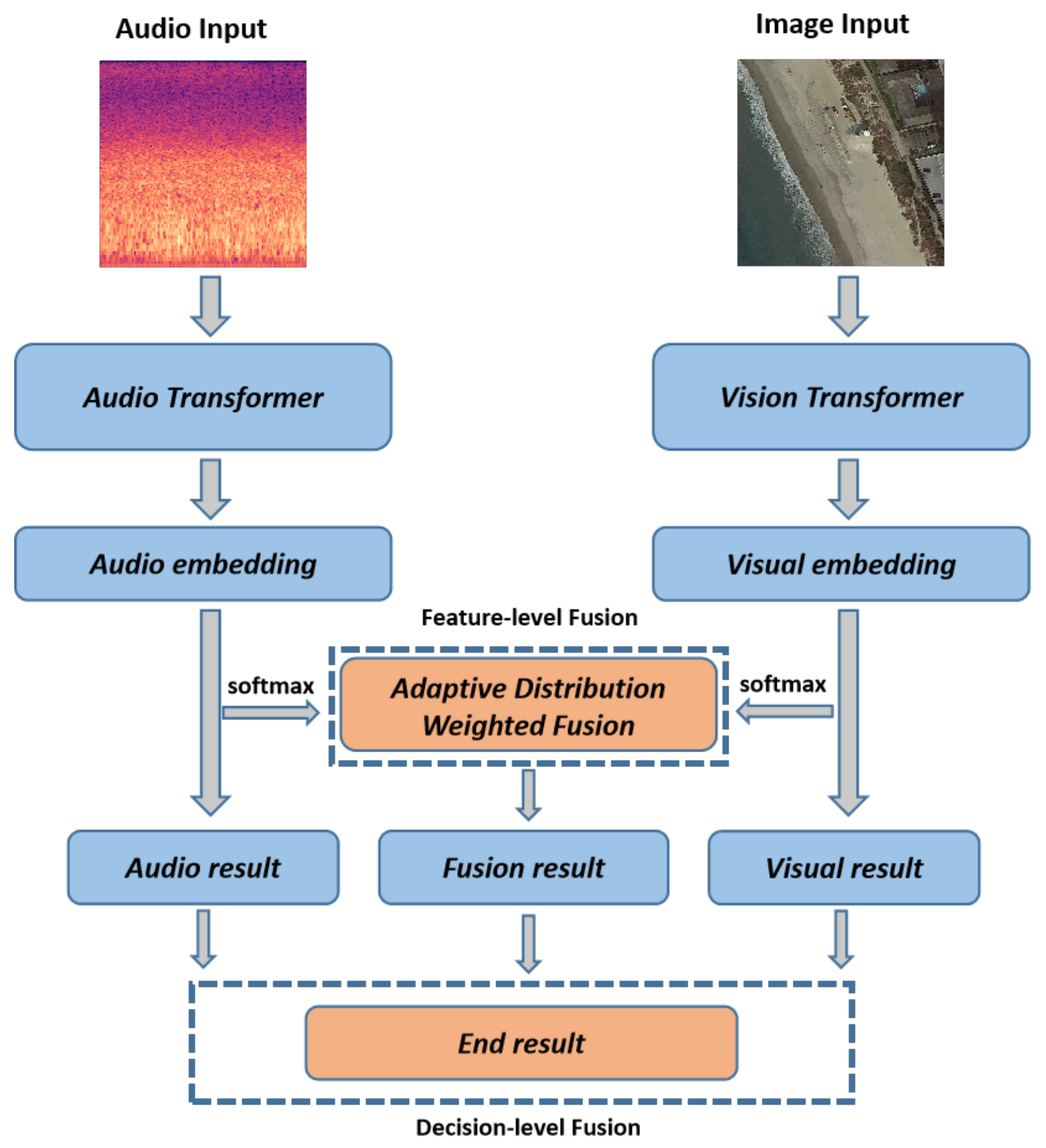
In this paper, we propose a novel two-stage fusion-based multimodal audiovisual classification network, aiming to explore the potential of using remote sensing images and ground environment audio for multimodal remote sensing scene classification. The audio, vision, and fusion modules make up the network. By combining ground environment audio and remote sensing aerial images, we can obtain more-accurate audiovisual scene classification results. The resilience of the classification method may also be improved via multimodal fusion, allowing it to perform well in challenging and noisy conditions. The following are the primary contributions of this study:

• A Two-stage Fusion-based Audiovisual Classification Network (TFAVCNet) was designed in this paper. We simultaneously used ground environment audio and remote sensing images to solve the task of remote sensing audiovisual scene classification in order to enhance the performance of single-mode remote sensing scene classification.
• The proposed approach makes use of two separate networks, which were, respectively, trained on audio and visual data, so that each network specialized in a given modality. We constructed the Audio Transformer (AiT) model to extract the time-domain and frequency-domain features of the audio signals.
• In the fusion module, we propose a two-stage hybrid fusion strategy. During the feature-level fusion stage, we propose the adaptive distribution weighted fusion to obtain the fusion embedding. In the decision-level fusion stage, we retained the single-mode decision results for both images and audio and weighted them with the feature fusion results.

This paper is organized as follows: Section 2 presents the related work. Section 3 presents the overall framework of the proposed audiovisual remote sensing scene classification network, as well as the audio module, visual module, and two-stage hybrid fusion strategy. Section 4 describes the details and results of each part of the performed experiments. Section 5 summarizes the paper and details the outlook for future research work.

2. Related Works

In recent years, researchers have paid close attention to the fusion of multimodal data for remote sensing scene classification. This section, divided into three parts, provides a brief overview of related work in the fields of audiovisual learning, remote sensing scene classification, and multimodal fusion in remote sensing.

2.1. Audiovisual Learning

Using both visual and audible information, audiovisual learning is a multimodal teaching and learning approach. As computer vision and voice processing have developed quickly over the past several years, more and more academics have focused on audiovisual learning and made impressive strides in a variety of tasks and applications. In order to give more thorough and precise scene understanding and event identification skills, audiovisual learning may combine the auditory aspects of speech signals with visual data from movies, such as face expressions and lip movements. Prominent results include the following: the introduction of visual modalities allows audiovisual separation and localization, i.e., the separation of specific sounds emanating from corresponding objects or the task of localizing sounds in visual modalities based on audio input [38,39]; the global semantic relationship among them, using the semantics provided by visual information, to improve the recognition performance of audiovisual speech recognition tasks [40,41,42,43]; based on one of the modalities to synthesize another modal cross-modal audiovisual generation task [44,45,46,47]; and audiovisual retrieval tasks that use audio or images to search for counterparts in another modality [48,49].

A wide range of applications for audiovisual learning exist outside of the domains of computer vision and voice processing. It may be used, for instance, in fields like robotic learning, intelligent monitoring, computer–human interaction, and virtual reality. In order to learn and comprehend remotely sensed audiovisual situations more effectively, we used the complementary nature of visual and aural information in this research.

2.2. Remote Sensing Multi-Modal Fusion Strategy

Given that sight and hearing are two of the five senses through which humans perceive the world, methods in both domains have advanced, giving rise to the emerging field of multimodal analysis. With the increasing availability of geotagged data from various sources, modes, and perspectives, facilitated by public audio libraries (e.g., Freesound, radio aporee) and mapping software (e.g., Google Maps 11.102.0101, Google Street View 2.0.0.484371618), the collection of such data has become more straightforward.

In general, multi-modal fusion methods can be roughly divided into three categories: data-level, feature-level, and decision-level fusion [50]. In the domain of remote sensing, data-level multimodal fusion has primarily been a focal point in early research endeavors. Data-level fusion methods typically involve the integration of raw or preprocessed data. Jakub Nalepa [51] used machine learning and advanced data analytics for multispectral and hyperspectral image processing. Mangalraj et al. [52] studied in detail the effectiveness of image fusion based on Multi-Resolution Analysis (MRA) and Multi-Geometric Analysis (MGA) and the impact of the corresponding fusion modes in retaining the required information. Another frequently employed approach is feature-level fusion, which involves the combination of intermediate features extracted from various modalities [53,54]. Lin et al. [55], inspired by the success of deep learning in face verification, proposed the Where-CNN method, demonstrating the effectiveness of Where-CNN in finding matches between street views and bird’s-eye view images. Workman et al. [56] combined overhead and ground images in an end-to-end trainable neural network that uses kernel regression and density estimation to convert features extracted from ground images into dense feature maps for estimating geospatial functions such as population density, land cover, or land use. Feature-level fusion methods tend to yield positive outcomes when the information supplied by different modalities in multimodal data demonstrates a substantial degree of correlation and consistency.

Decision-level fusion employs various fusion rules to aggregate predictions from multiple classifiers, each derived from a separate model. By using methods like weighted summation, voting, or probability-based approaches [57,58], decision fusion aims to enhance the reliability and consistency of classification results. Hu et al. [59] developed a method that combines the physical characteristics of remote sensing data (i.e., spectral information) and the social attributes of open social data (e.g., socioeconomic functions), to quickly identify land use types in large areas and tested its effectiveness in Beijing. Liu et al. [60] proposed a novel scene classification framework to identify major urban land use types at the traffic analysis area level by integrating probabilistic topic models and support vector machines. It plays a crucial role in improving and balancing different modalities, especially when the decision outcomes of these modalities differ significantly from one another or when there is little correlation between them [61].

For the purpose of fully utilizing the benefits of multimodal data and enhancing the performance of remote sensing audiovisual scene classification, we used feature fusion and decision fusion to process the features and decision results of audiovisual data.

3. Methods

3.1. Overall Framework

As depicted in Figure 1, we present a novel framework aimed at enhancing the performance of remote sensing scene classification. Our approach, known as the Two-stage Fusion-based Audiovisual Classification Network (TFAVCNet), serves as the foundation of this method. In the first step, the audio module extracts audio embeddings from the audio input, represented by an audio spectrogram computed from the raw audio file. Simultaneously, the image module extracts the visual embedding from the image input, consisting of a remote sensing aerial image. Subsequently, in the feature-level fusion stage, the adaptive distribution weighted fusion module combines the audio and visual embeddings. Importantly, in the decision-level fusion stage, we preserve the results of single-mode decisions to effectively retain the original information from each modality. In the final step, the results of audio-, visual-, and feature-level fusion undergo a second-stage weighted fusion process, culminating in classification via the Softmax function. The subsequent subsections provide a more-detailed exploration of each module.

3.2. Audio Module

As shown in Figure 2, the CNN structure, or the CNN combined with a the basic self-attention mechanism, is the typical foundation for traditional acoustic scene-classification algorithms. For tasks involving natural language processing, Transformer was initially proposed. For the implementation of our audio module, we adopted a Transformer-based model from the field of visual processing, in contrast to the prior usage of the CNN architecture or a combination of the CNN and self-attention mechanisms for audio scene classification [16,62,63]. We constructed the Audio Transformer (AiT) model to extract the time-domain and frequency-domain features of the audio signals, on which we carried out the tasks for audio scene classification.

Figure 3 displays our audio module. The AiT and ViT share similar foundational structures, as both are non-convolutional models primarily constructed using attention mechanisms. However, a significant distinction arises in their respective input requirements. While the ViT is designed to process three-channel images, the AiT operates on a single-channel log-Mel spectrogram. To accommodate this different input format, we averaged the channel weights of the patch-embedding layer. Furthermore, given the utilization of pre-trained weights, the input dimensions of the log-Mel spectrogram (batch_size, hop_length, n_mels) do not align with the fixed input size of the ViT-B (batch_size, 384, 384).Therefore, we rescaled the position embedding of the ViT according to the dimension of the spectrogram. First, the audio file’s log-Mel spectrogram is calculated and used as the patch embedding layer’s input. An audio file with a length of t seconds will receive an audio input with a size of (batch_size, n_mels, hop_length). Please note that the audio files referenced in this context pertain specifically to ground environment sounds, and each of them corresponds directly to a corresponding remote sensing aerial image. For a more-in-depth explanation of the audio spectrogram computation, please refer to the Experiments Section 4.6. The spectrogram is then divided into a series of patches, each of which is fed into a linear projection layer to produce patch embeddings (batch_size, n_patches, 768). After that, we added learnable positional embeddings and categorical variable $CLS$ tokens at the start of the patch-embedding sequence before feeding them into the Transformer encoder layer. We averaged the two $CLS$ tokens (classification token and distillation token) to create an audio spectrogram representation in the Transformer encoder using the DeiT-B pre-trained weights from ImageNet. In order to obtain the audio_result vector, we must first obtain the output of the audio module ($CLS$ token) as the feature of the audio spectrogram (audio embedding), input it into a fully connected layer with Softmax activation, then map the audio embedding to the label for classification.

According to strict definitions, the patch-embedding layer can be thought of as a single convolutional layer with a big kernel and stride size, while the projection layer in each Transformer block is comparable to a 1 × 1 convolution. The design deviates from typical CNNs, which have many layers and tiny kernel and stride sizes. In order to separate these Transformer models from the CNNs, they are typically referred to as convolution-free.

3.3. Visual Module

To learn image representations appropriate for this dataset, we specifically fine-tuned on the images in the target dataset using the weights of the ViT [64] model that have already been trained on ImageNet. We obtained four variants of the Vision Transformer by assigning various values to the block numbers and token dimensions: ViT-T, ViT-S, ViT-B, and ViT-L, where T, S, B, and L correspond to the number of parameters (i.e., tiny, small, base, and big). As the ViT-B has a reasonable balance between performance and model size, it serves as the foundation of our methodology there. The ViT separates the input image into various patches, projects each patch into a fixed-length vector, and then, passes the vector to the Transformer. As with the original Transformer, the ensuing encoder operations are identical. However, in order to account for the classification of the images, a specific token ($CLS$) is added to the input sequence, and the output corresponding to the token is the final category prediction.

As shown in Figure 4, each image will produce 196 patches when divided into groups of patches of a specific size; this means that the input sequence length is 196 and the dimension of each patch is 768. The addition of the $CLS$ token and position embedding is required prior to entering the Transformer encoder. Position embedding is a straight add-on token, and the token is concatenated with the token created from the previous image. The shape after splicing the $CLS$ token is currently (197, 768), so the shape of the position embedding is also (197, 768). Following feature extraction by the Multi-Layer Perceptron (MLP) and encoding by the multi-head self-attention module, the output ($CLS$ token) is regarded as the feature (visual embedding) of the image. The visual embedding is mapped to the label for classification to obtain the visual_result vector.

In the vision module, we are able to extract more-significant and -expressive features from images by utilizing the ViT model and the transfer learning method. Such feature representations can aid in improving our comprehension of the information contained in images and can deliver more-precise data for the upcoming scene classification tasks.

3.4. Two-Stage Hybrid Fusion Strategy

Integrating data from various modalities is the aim of multimodal fusion. Early fusion (feature-level fusion) and late fusion (decision-level fusion) are the two primary multimodal fusion strategies. However, because the sparsity of the features extracted by various modalities may differ, their distributions may differ significantly. Therefore, it may not be possible to achieve the best fusion results by simply concatenating multimodal features into an input-level joint feature vector. Additionally, because decision-level fusion does not take into account the relationship between feature sets, it is not possible to fully utilize the similarity and complementarity of features, and it may not produce satisfactory fusion results.

As shown in Figure 5, we propose a two-stage hybrid fusion strategy, which consists of feature-level fusion and decision-level fusion. This module fuses information from both audio and visual modalities in two stages and trains jointly to achieve a more-robust solution.

In the feature-level fusion stage, we designed the adaptive distribution weighted fusion module to obtain fusion embedding. First, we calculated the Softmax results of audio embedding and visual embedding. Both embeddings share the same dimensions (batch_size, 768). The normalized weight (or importance) of the channel is calculated by computing the Softmax of the i-th channel of embedding [65], as shown in Equation (1).

$$S\left(e_i\right)=\frac{exp\left(e_i\right)}{{\sum }_{i}exp\left(e_i\right)}$$

(1)

where $e_i$ is the i-th channel of embedding.

Then, calculate the weight of audio embedding ($f_1$) and visual embedding ($f_2$) for fusion embedding ($f_3$) by calculating the matrix kernel norm ($\Vert S{\Vert }_{*}$). Finally, the weight of the embedding is obtained by taking the weighted average of the nuclear norm. The calculation formula is given by Equations (2) and (3).

$$W_1=\frac{\phi (\Vert S{\left(e_i\right)}^1{\Vert }_{*})}{\phi (\Vert S{\left(e_i\right)}^1{\Vert }_{*})+\phi (\Vert S{\left(e_i\right)}^2{\Vert }_{*})}$$

(2)

$$W_2=\frac{\phi (\Vert S{\left(e_i\right)}^2{\Vert }_{*})}{\phi (\Vert S{\left(e_i\right)}^1{\Vert }_{*})+\phi (\Vert S{\left(e_i\right)}^2{\Vert }_{*})}$$

(3)

where $S{\left(e_i\right)}^j,j\in [1,2]$ is the weight after the Softmax operation for the feature $f_j,j\in [1,2]$ and $\phi (·)$ can be any arbitrary functions; we will discuss the effect of different function settings on the results in detail in the later experimental part. The final fusion embedding is then given by $f=W_1\times f_1+W_2\times f_2$.

After obtaining the audio, visual, and fusion embeddings, map the three embeddings to the labels for classification using a fully connected layer with Softmax activation to produce the audio result, visual result, and fusion result vectors, each of which has a batch size of 13.

We weighted and fused the output results of the audio module, visual module, and feature-level fusion stage in the decision-level fusion stage to maximize the use of the two types of single-mode information and weighted fusion information. These outputs are all probability distributions that were obtained using a Softmax activation function on a fully connected layer. The calculation process is shown in Equation (4). $\varphi (·)$ can be any arbitrary functions; we will discuss the effect of different function settings on the results in detail in the later experimental part.

$$R=\varphi (R_1,R_2,R_3)$$

(4)

4. Experiments

In this section, we evaluate our audio module, visual module, and two-stage hybrid fusion strategy on a publicly available dataset for remote sensing audiovisual scene classification. We first introduce the dataset that will be used, as well as the experimental setup and evaluation metrics. Second, we compared these three modules to current methods and experimentally show their efficacy.

4.1. Dataset

The audiovisual dataset we used is the AuDio Visual Aerial sceNe reCognition datasEt (ADVANCE) [66], a multimodal learning dataset, which aims to explore the contribution of both audio and conventional visual messages to scene recognition. This dataset in summary contains 5075 pairs of geotagged aerial images and sounds, classified into 13 scene classes, i.e., airport, sports land, beach, bridge, farmland, forest, grassland, harbor, lake, orchard, residential area, shrubland, and train station. Some examples in the dataset are shown in Figure 6. The number of image–audio pairs in each scene is shown in

Table 1. ADVANCE dataset scene category distribution.

Scene Category of ADVANCE	Total
Airport	185
Beach	216
Bridge	280
Farmland	430
Forest	862
Grassland	150
Harbor	508
Lake	357
Orchard	207
Residential	1056
Shrubland	405
Sports land	159
Train station	260

.

4.2. Experimental Setup and Evaluation Metrics

All experiments were implemented using Pytoch 1.12. The models were trained on an NVIDIA RTX 3080 (12 GB) GPU in a single machine. The details during training were as follows. In the audio module, we used the pretrained weights of a DeiT-base 384 [67], which is trained with CNN knowledge distillation, with 384 × 384 images, and has 87M parameters. In the visual module, we used a ViT-B/16 [64] (with 70 M parameters) as the backbone. We removed the original fully connected layers of the two Transformers. In addition, the pretrained parameters of ImageNet-21K were loaded on the DeiT-base 384 and ViT-B/16 (except the fully connected layer). When training TFAVCNet, we chose the Adam optimizer with a relatively small learning rate of $1\times {10}^{-4}$ and a weight decay of $1\times {10}^{-3}$ to optimize the parameters of TFAVCNet, as both backbones have been pre-trained from external knowledge. In the optimizer, we improved the stability of the model by taking a 10-epoch warm-up strategy. Considering the limited GPU memory resource, we set the batch size to 64 for the audio experiment and to 32 for the image.

Splitting strategy: The ADVANCE dataset was employed for the evaluation, where 70% image–sound pairs were for training, 10% for validation, and 20% for testing. All the test results are the mean results of 10 splits in order to reduce random influence.

Evaluation metrics: To quantitatively evaluate the performance of each module, we adopted the weighted average precision, recall, and F-score metrics with the standard deviation (±STD) for the evaluation. The distribution of the data can have an impact on accuracy in tasks with imbalanced classes, as the model may be biased towards prediction if the number of samples from one class is significantly higher than the number of samples from another class. Most categories receive high accuracy ratings, while minority categories receive an insufficient performance evaluation. Metrics like the precision, recall, and F-score may be more useful in this situation because they give more in-depth information to analyze the model’s performance across various categories:

• The accuracy of model predictions is determined by the precision. It shows how many of the samples that the model predicted to be positive are actually positive.
• Another crucial evaluation metric is the recall, which is used to determine how well the model is able to identify all real positive examples. A high recall means that the model can capture positive examples more accurately.
• The F-score combines the precision and recall to provide an indicator for comprehensively evaluating model performance. The F-score is the weighted average of the precision and recall, where the weight factor can be adjusted according to the task requirements. The most-common F-score is the F1-score, which gives equal weight to the precision and recall.

4.3. Audio Experiments

Here, we compare the results of four schemes, ADVANCE [66], SoundingEarth [68], attention + CNN, and AiT, to demonstrate the effectiveness of the schemes based only on Transformer. Among them, the acoustic characteristics of the four schemes are common (use the log-Mel spectrogram). The audio path of the ADVANCE solution uses the AudioSet pre-trained ResNet-50 to model the sound content. The second solution uses batch triplet loss, which has the advantage of combining classical triplet loss training with recent contrastive learning methods. The third scheme consists of a single layer of self-attention and four layers of convolution. The fourth option is the audio Transformer introduced in Section 3.2.

In order to prevent purely memorizing the input data and introducing more diversity into the training samples, we used frequency mask and time mask data augmentation [69] for the audio spectrogram, so that the AiT model can learn more-robust feature representations, thereby improving the generalization performance on the validation dataset. Specifically, before extracting the spectrogram features, we applied the FrequencyMasking (freqm) and TimeMasking (timem) transformations. The parameters, freqm and timem, represent the respective widths of the continuous frequency interval and time window to be masked. In addition, we also normalized the feature dimension of the spectrogram, so that the dataset was normalized to 0 mean and standard deviation.

Table 2. Results (%) ± STD of the experiments on audio systems.

Methods	Precision	Recall	F1-Score
ADVANCE (ResNet-50) [66]	30.46 ± 0.66	32.99 ± 1.20	28.99 ± 0.51
SoundingEarth (ResNet-18) [68]	37.91 ± 0.31	38.36 ± 0.25	37.69 ± 0.19
SoundingEarth (ResNet-50) [68]	39.13 ± 0.22	39.96 ± 0.14	39.01 ± 0.17
Attention + CNN	33.41 ± 0.21	34.42 ± 0.41	33.56 ± 0.24
AiT (Ours)	41.8 ± 0.15	42.8 ± 0.61	41.9 ± 0.11

shows the results of different audio system approaches. We can observe that the method using the attention + CNN architecture is superior to the baseline (ADVANCE) scheme based on the CNN architecture on all three indicators. Specifically, the results of the attention + CNN architecture (33.56% ± 0.24 on the F1-score) are 4.57% higher than the ADVANCE method (28.99% ± 0.51 on the F1-score) using only CNN, but it has no advantage or is even worse than the SoundingEarth scheme. According to the preliminary analysis, the attention + CNN structure does not receive any additional dataset pre-training, whereas the SoundingEarth model is pre-trained on a large audiovisual dataset. From the AiT scheme, we can observe that, in the case of using a pre-trained model, only the Transformer-based method (41.9% ± 0.11 on the F1-score) is 2.89% higher than the ADVANCE and SoundingEarth methods (39.01% ± 0.17 on the F1-score), which also use the transfer learning method.

The confusion matrix for our the audio classification model AiT is shown in Figure 7. When only audio samples were used in the training, the ability to classify audio scenes was poor. Although forest and residential scenes with a large number of samples had better classification results, this also led to natural scenes (such as shrubland, orchard, and grassland) and scenes of human life (such as farmland and sports land) having poor classification results. As a consequence, there were some limitations when classifying scenes solely based on land ambient audio.

4.4. Image Experiments

This experiment did not establish a new image scene classification model. We chose to use the ViT-B/16 classification model, which is effective in the field of image classification, with an appropriate number of model parameters. Here, we compare the results of the ADVANCE scheme, the SoundingEarth scheme, and the Vision Transformer architecture. In addition, the pretrained parameters of ImageNet-21K were loaded onto the ViT-B/16 (except the fully connected layer). During fine-tuning, we normalized all images and used random repositioning cropping, random horizontal flipping, random adjustment of image brightness and contrast, and other data-enhancement techniques.

The visual pathway in the ADVANCE solution employs a pre-trained ResNet-101 from AID. Likewise, the second solution utilizes a ResNet architecture, but with a distinction: it employs pre-trained ResNet-18 and ResNet-50 models using the SoundingEarth dataset. In the third approach, we opted for the ViT-B/16 for comparative purposes.

Table 3. Results (%) ± STD of the experiments on visual systems.

Methods	Precision	Recall	F1-Score
ADVANCE (ResNet-101) [66]	74.05 ± 0.42	72.79 ± 0.62	72.85 ± 0.57
SoundingEarth (ResNet-18) [68]	87.09 ± 0.19	87.07 ± 0.11	86.92 ± 0.16
SoundingEarth (ResNet-50) [68]	83.97 ± 0.15	83.88 ± 0.14	83.84 ± 0.17
ViT-B/16 (Ours)	87.64 ± 0.38	87.52 ± 0.49	87.61 ± 0.41

, shows the results of different image system methods. We can observe that the method of the SoundingEarth scheme architecture (86.92% ± 0.16 on the F1-score) performed 14.07% higher than the baseline (ADVANCE) scheme (72.85% ± 0.57 on the F1-score). One of the most-straightforward explanations is that, despite their models being pre-trained on large-scale aerial image datasets, the dataset scale varies. The SoundingEarth scheme employs a dataset that is five-times larger than that of ADVANCE (AID comprises over 10,000 aerial scene images, while SoundingEarth boasts more than 50,000 overhead imagery samples). The Vision Transformer introduces a self-attention mechanism, which can effectively capture different positions in the image dependencies between and model global information. Although it was not pre-trained on a large-scale aerial scene images dataset, it still showed its efficient scene classification performance (87.61% ± 0.41 on the F1-score).

The confusion matrix for our image classification model is shown in Figure 8. Scene classification using images is better than scene classification using audio. The figure shows that, first, there were much fewer test samples that were incorrectly classified, and in some scenes (like beach, forest, harbor, residential, and train station), there were very few misclassified samples. Second, the scenes farmland, orchard, and shrubland were where the misclassified test samples were most-frequently found. In the scene, eight samples of farmland were incorrectly classified as grassland, nine samples of orchard were incorrectly classified as forest, and eight samples of shrubland were incorrectly classified as forest. Eight samples from sports land were incorrectly classified as residential for the same issue, and six samples from lake were incorrectly classified as harbor.

4.5. Audiovisual Experiments

Here, we compare the results of ADVANCE [66], SoundingEarth [68], and our two-stage hybrid fusion strategy and show the quantitative results of different fusion strategies on three metrics (precision, recall, F1-score). The ADVANCE scheme transfers sound event knowledge to aerial scene recognition tasks to improve scene recognition performance. The SoundingEarth solution learns semantic representation between the audio and image modalities through self-supervised learning. Next, in our two-stage hybrid fusion schemes, we selected the $max\left(\right)$ and $sum\left(\right)$ functions to determine $\phi (·)$ and $\varphi (·)$ for feature fusion and decision fusion.

From

Table 4. Results (%) ± STD of the experiments on audiovisual systems.

Methods	Precision	Recall	F1-Score
ADVANCE (ResNet + Cross-Task Transfer) [66]	75.25 ± 0.34	74.79 ± 0.34	74.58 ± 0.25
SoundingEarth (ResNet-18) [68]	89.59 ± 0.27	89.52 ± 0.29	89.5 ± 0.12
SoundingEarth (ResNet-50) [68]	88.9 ± 0.21	88.85 ± 0.34	88.83 ± 0.27
TFAVCNet (Ours)	89.9 ± 0.14	89.85 ± 0.36	89.83 ± 0.21

, the following observations can be made. First, audiovisual experiments can achieve better results than those based only on audio or visual information, suggesting that fusing information from the audio and visual modalities can improve single-mode classification. Secondly, for the comparison of the fusion methods, our two-stage fusion strategy further improved the effect compared with the ADVANCE method and SoundingEarth method, which only use feature fusion.

The confusion matrix of our two-stage hybrid fusion strategy’s classification results is shown in Figure 9. For the majority of categories, we can see that the result of classification tended to be good. In certain scenes (forest, harbor, residential), it worked flawlessly. Grassland and orchard were the scenes with the worst classification. In the test set for grassland, six samples were classified as forest, six as shrubland, and three as farmland; in the test set for orchard, eight samples were classified as forests and three were classified as farmland. The dataset’s obvious long tail distribution and the insufficient sample size for the grassland and orchard scenes prevented the model from learning more-useful distinguishing features, according to preliminary analysis. The fact that the scene’s audio events were too similar could also be a factor. In the grassland, forest, and shrubland scenes, we discovered that there were numerous similar sound events, such as birdsong, water, etc., through manual inspection. The vast amounts of green vegetation in both scenes, which are indistinguishable to humans, further resembled one another, creating a visual similarity between the two.

4.6. Log-Mel Spectrogram

Different acoustic features will have different effects on the accuracy of scene classification. Here, we chose the log-Mel spectrogram, which is widely used in the field of speech and sound processing.

The log-Mel spectrogram provides more-detailed spectrum information than the traditional spectrogram. It is divided into frames on the time axis, and each frame represents the energy distribution of different frequencies over a period of time. The purpose of logarithmic transformations, usually applied to Mel spectrograms, is to enhance details in low-energy regions such that the features are more evenly distributed on a logarithmic scale. The calculation process of the log-Mel spectrogram is shown in Formula (5).

$$Mel\left(f\right)=2595*{log}_{10}(1+\frac{f}{700})$$

(5)

where f is the frequency expressed in Hertz and $Mel\left(f\right)$ is the corresponding Mel frequency.

In addition, we performed some experimental analysis on two important parameters in the calculation of the spectrogram: hop length and number of Mel filters, to determine the optimal hyperparameters. The results are shown in

Table 5. The experimental results of the hop length and the number of Mel filters of the log-Mel spectrogram feature.

Log-Mel Spectrogram Parameters	Size	Accuracy
Hop Length 1	300	0.3235 ± 0.0019
	400	0.3288 ± 0.0016
	500	0.3275 ± 0.0008
Number of Mel Filters 2	32	0.3425 ± 0.0091
	64	0.3494 ± 0.0085
	128	0.3571 ± 0.0039

¹ Hop length: number of samples between consecutive analysis frames. Smaller frame shifts provide better temporal resolution, but also lead to increased computation. ² Number of Mel filters: the number of Mel frequency bands. A larger number of filters can provide better frequency resolution, but also increases computational complexity.

.

Hop length is measured on samples here, and 441 samples corresponded to 10 ms at a sampling rate of 44,100. In this experiment, we can see that a hop length of 400 samples (about 10 ms) had a higher average accuracy overall. Hop length is important, because it directly affects how “wide” the image is, so while a hop length of 5 ms might have a slightly higher accuracy than 10 ms, the images will be twice as large and, therefore, take up twice as much GPU memory.

If hop length determines the width of the spectrogram, then the height is determined by the number of Mel filters. After first producing a regular STFT using an FFT size of, say, 2048, the result is a spectrum with 1025 FFT bins, varying over time. When we convert to a Mel spectrogram, those bins are logarithmically compressed down to n_mels bands. This experiment showed that 32 is definitely too few, but other than that, it did not affect the accuracy too much. A value of 128, which is the default with the baseline, gave the highest mean accuracy.

Figure 10 shows the log-Mel spectrogram for the two audio scene classes we created using the librosa library, with hop_length set to 400 and the number of Mel filters set to 128. The plotted log-Mel spectrogram shows the characteristics of the audio signal in time and frequency. Some information can be observed from the spectrogram:

• Time information: Each time step on the x-axis corresponds to an audio frame, which is the time axis of the audio signal. The audio’s temporal development is visible.
• Frequency information: The frequency band of the Mel filter is shown on the y-axis, which is typically scaled in the Mel frequency. The Mel frequency is a frequency scale that is connected to human auditory perception and more closely resembles the features of the auditory system in humans.
• Energy information: Each time frame’s logarithmic energy for each Mel frequency band is represented by a different color. The relative strength of various frequency components in the audio signal can be represented using this.

For example, contrast the spectrograms of the 07497_4.wav airport scene and the 00095.wav beach scene. Intermittent high-frequency, high-intensity sounds can be seen in the high-frequency portion of the airport scene spectrogram (the darkest part at the top); medium-to-high-intensity sounds can be seen in the middle portion (the dark, large area in the middle of the spectrogram); there is obviously medium–low intensity sound in the middle and rear portions of the low-frequency portion (the orange–white part at the bottom). By manually listening to the 07497_4.wav file, we can clearly hear the airport broadcast beginning at the third second in the scene (corresponding to the orange part starting at the third second in the spectrogram), as well as the noisy human conversation in the scene (corresponding to the darker, high-intensity portion of the spectrogram). An obvious low-intensity (large areas of orange–yellow) sound in the middle and low frequencies (low-intensity sounds are mainly shown in the middle and lower parts of the spectrogram) can be seen in the spectrogram of the beach scene. By manually listening to the 00095.wav file, we can identify the long-lasting, low-intensity ocean waves that are audible in this scene. Additionally, the spectrogram makes it easy to see the audio noise (possibly wind sound) and the brief burst of bird calls in the first few seconds.

Different areas in the spectrogram are represented by the frequency components, energy distribution, time-domain characteristics, background noise, and other information of the various sounds in the environment. It is crucial for subsequent models to achieve good classification performance to choose an appropriate audio feature extraction technique by choosing better hyperparameters.

4.7. Fusion Strategy Experiments

This section chooses various $\phi (·)$ and $\varphi (·)$ functions to find the best function settings for feature fusion and decision fusion. On the three metrics (precision, recall, and F1-score), as shown in

Table 6. Results (%) ± STD of the experiments on fusion strategy.

Methods	Precision	Recall	F1-Score
Feature-Level (ADVANCE) [66]	73.93 ± 0.8	72.91 ± 0.74	72.71 ± 0.76
Feature-Level ($\phi (·)=mean$)	79.12 ± 0.27	78.42 ± 0.22	79.41 ± 0.27
Feature-Level ($\phi (·)=max$)	83.91 ± 0.33	83.02 ± 0.38	83.02 ± 0.35
Feature-Level ($\phi (·)=sum$)	84.05 ± 0.30	83.56 ± 0.39	83.72 ± 0.42
Feature-Level ($\phi (·)=max+sum$)	85.21 ± 0.98	84.76 ± 0.46	84.74 ± 0.31
Decision-Level ($\varphi (·)=mean$)	79.96 ± 0.52	79.75 ± 0.61	79.93 ± 0.49
Decision-Level ($\varphi (·)=max$)	87.02 ± 0.47	87.75 ± 0.38	87.06 ± 0.25
Decision-Level ($\varphi (·)=sum$)	86.64 ± 0.25	86.61 ± 0.34	86.56 ± 0.24
Decision-Level ($\varphi (·)=max+sum$)	88.12 ± 0.23	88.31 ± 0.31	88.02 ± 0.35
Proposed	89.9 ± 0.14	89.85 ± 0.36	89.83 ± 0.21

, we used the average, max, and sum functions to show the quantitative results of various fusion strategies.

The following observations can be made. First of all, the baseline (ADVANCE scheme) uses feature splicing in the feature-level fusion method to combine audio features and image features. This straightforward fusion approach is not superior to the single-mode image method. When using a two-stage hybrid fusion strategy, the fusion’s performance will increase and its constituent features will become more abstract. Second, in feature-level fusion and decision-level fusion, the performance of the $max$ and $sum$ functions for the selection of the $\phi (·)$ and $\varphi (·)$ functions was nearly identical, and both were superior to the $mean$ function. The most-ideal strategy is when the $max+sum$ function setting was used. Last but not least, the proposed strategy was actually a result of feature enhancement performed in two steps. The weights of the audio and the image that determine the results of classification were not equal under the two stages’ weighting; instead, the more-significant party was given a greater weight.

5. Conclusions

Traditional remote sensing scene classification tasks have been broadened by ground environment audio and remote sensing aerial images. In this study, we presented TFAVCNet, a two-stage fused-based multimodal audiovisual classification network for tasks involving scene classification in audiovisual remote sensing. TFAVCNet is made up of an audio module, a vision module, and a fusion module, which effectively combine the acoustic and visual modalities, and achieves state-of-the-art performance. In addition, in order to extract valuable ground environment audio information, we designed a Transformer-based Audio Transformer (AiT) network, which is different from the previous CNN or a CNN combined with a self-attention network. Additionally, in the fusion module, we designed an adaptive distributed weighted fusion module to obtain fusion embedding. Especially in the decision fusion module, we retained the single-mode decision results for both images and audio and weighted them with the feature fusion results.

There is still much research to be performed in the area of remote sensing scene classification based on audiovisual fusion. Firstly, the availability of publicly accessible audiovisual multimodal datasets for remote sensing tasks is limited, and there is an urgent requirement for extensive remote sensing audiovisual multimodal datasets to support relevant research initiatives. Moreover, it is essential to explore methods for effectively modeling single-mode information when integrating visual and auditory data. There is a need to investigate how to extract more-valuable supervisory information from the coarse-level congruence of the visual and auditory modalities when they are combined. Finally, more-effective fusion methods should be designed to build the correlation between them. Because information is different, some have more information, some have less information, and the synchronicity between them is different.

References

1. Wang, M.; Zhang, X.; Niu, X.; Wang, F.; Zhang, X. Scene classification of high-resolution remotely sensed image based on ResNet. J. Geovis. Spat. Anal. 2019, 3, 16. [Google Scholar] [CrossRef]
2. Shabbir, A.; Ali, N.; Ahmed, J.; Zafar, B.; Rasheed, A.; Sajid, M.; Ahmed, A.; Dar, S.H. Satellite and scene image classification based on transfer learning and fine tuning of ResNet50. Math. Probl. Eng. 2021, 2021, 5843816. [Google Scholar] [CrossRef]
3. Zhou, Y.; Chen, P.; Liu, N.; Yin, Q.; Zhang, F. Graph-Embedding Balanced Transfer Subspace Learning for Hyperspectral Cross-Scene Classification. IEEE J. Sel. Top. Appl. Earth Obs. Remote Sens. 2022, 15, 2944–2955. [Google Scholar] [CrossRef]
4. Chen, L.; Cui, X.; Li, Z.; Yuan, Z.; Xing, J.; Xing, X.; Jia, Z. A new deep learning algorithm for SAR scene classification based on spatial statistical modeling and features re-calibration. Sensors 2019, 19, 2479. [Google Scholar] [CrossRef] [PubMed]
5. Wang, Q.; Liu, S.; Chanussot, J.; Li, X. Scene Classification With Recurrent Attention of VHR Remote Sensing Images. IEEE Trans. Geosci. Remote Sens. 2019, 57, 1155–1167. [Google Scholar] [CrossRef]
6. Li, B.; Guo, Y.; Yang, J.; Wang, L.; Wang, Y.; An, W. Gated Recurrent Multiattention Network for VHR Remote Sensing Image Classification. IEEE Trans. Geosci. Remote Sens. 2022, 60, 5606113. [Google Scholar] [CrossRef]
7. Wellmann, T.; Lausch, A.; Andersson, E.; Knapp, S.; Cortinovis, C.; Jache, J.; Scheuer, S.; Kremer, P.; Mascarenhas, A.; Kraemer, R.; et al. Remote sensing in urban planning: Contributions towards ecologically sound policies? Landsc. Urban Plan. 2020, 204, 103921. [Google Scholar] [CrossRef]
8. Zhang, T.; Huang, X. Monitoring of Urban Impervious Surfaces Using Time Series of High-Resolution Remote Sensing Images in Rapidly Urbanized Areas: A Case Study of Shenzhen. IEEE J. Sel. Top. Appl. Earth Obs. Remote Sens. 2018, 11, 2692–2708. [Google Scholar] [CrossRef]
9. Ghazouani, F.; Farah, I.R.; Solaiman, B. A Multi-Level Semantic Scene Interpretation Strategy for Change Interpretation in Remote Sensing Imagery. IEEE Trans. Geosci. Remote Sens. 2019, 57, 8775–8795. [Google Scholar] [CrossRef]
10. Mesaros, A.; Heittola, T.; Virtanen, T. Acoustic Scene Classification: An Overview of Dcase 2017 Challenge Entries. In Proceedings of the 2018 16th International Workshop on Acoustic Signal Enhancement (IWAENC), Tokyo, Japan, 17–20 September 2018; pp. 411–415. [Google Scholar] [CrossRef]
11. Valenti, M.; Diment, A.; Parascandolo, G.; Squartini, S.; Virtanen, T. DCASE 2016 Acoustic Scene Classification Using Convolutional Neural Networks. In Proceedings of the Detection and Classification of Acoustic Scenes and Events 2016 Workshop (DCASE2016), Budapest, Hungary, 3 September 2016; pp. 95–99. [Google Scholar]
12. Barchiesi, D.; Giannoulis, D.; Stowell, D.; Plumbley, M.D. Acoustic Scene Classification: Classifying environments from the sounds they produce. IEEE Signal Process. Mag. 2015, 32, 16–34. [Google Scholar] [CrossRef]
13. Rybakov, O.; Kononenko, N.; Subrahmanya, N.; Visontai, M.; Laurenzo, S. Streaming Keyword Spotting on Mobile Devices. In Proceedings of the Interspeech 2020, Shanghai, China, 25–29 October 2020; pp. 2277–2281. [Google Scholar] [CrossRef]
14. Li, P.; Song, Y.; McLoughlin, I.; Guo, W.; Dai, L. An Attention Pooling Based Representation Learning Method for Speech Emotion Recognition. In Proceedings of the Interspeech 2018, Hyderabad, India, 2–6 September 2018; pp. 3087–3091. [Google Scholar] [CrossRef]
15. Kong, Q.; Cao, Y.; Iqbal, T.; Wang, Y.; Wang, W.; Plumbley, M.D. PANNs: Large-Scale Pretrained Audio Neural Networks for Audio Pattern Recognition. IEEE/ACM Trans. Audio Speech Lang. Process. 2020, 28, 2880–2894. [Google Scholar] [CrossRef]
16. Gong, Y.; Chung, Y.A.; Glass, J. PSLA: Improving Audio Tagging With Pretraining, Sampling, Labeling, and Aggregation. IEEE/ACM Trans. Audio Speech Lang. Process. 2021, 29, 3292–3306. [Google Scholar] [CrossRef]
17. Abeßer, J. A Review of Deep Learning Based Methods for Acoustic Scene Classification. Appl. Sci. 2020, 10, 2020. [Google Scholar] [CrossRef]
18. Ren, Z.; Kong, Q.; Han, J.; Plumbley, M.D.; Schuller, B.W. Attention-based Atrous Convolutional Neural Networks: Visualisation and Understanding Perspectives of Acoustic Scenes. In Proceedings of the ICASSP 2019-2019 IEEE International Conference on Acoustics, Speech and Signal Processing (ICASSP), Brighton, UK, 12–17 May 2019; pp. 56–60. [Google Scholar] [CrossRef]
19. Koutini, K.; Eghbal-zadeh, H.; Widmer, G. CP-JKU Submissions to DCASE’19: Acoustic Scene Classification and Audio Tagging with Receptive-Field-Regularized CNNS Technical Report. In Proceedings of the Detection and Classification of Acoustic Scenes and Events 2019, New York, NY, USA, 25–26 October 2019. [Google Scholar]
20. Basbug, A.M.; Sert, M. Acoustic Scene Classification Using Spatial Pyramid Pooling with Convolutional Neural Networks. In Proceedings of the 2019 IEEE 13th International Conference on Semantic Computing (ICSC), Newport Beach, CA, USA, 30 January–1 February 2019; pp. 128–131. [Google Scholar] [CrossRef]
21. Li, Z.; Hou, Y.; Xie, X.; Li, S.; Zhang, L.; Du, S.; Liu, W. Multi-level Attention Model with Deep Scattering Spectrum for Acoustic Scene Classification. In Proceedings of the 2019 IEEE International Conference on Multimedia & Expo Workshops (ICMEW), Shanghai, China, 8–12 July 2019; pp. 396–401. [Google Scholar] [CrossRef]
22. Wang, C.Y.; Santoso, A.; Wang, J.C. Acoustic scene classification using self-determination convolutional neural network. In Proceedings of the 2017 Asia-Pacific Signal and Information Processing Association Annual Summit and Conference (APSIPA ASC), Kuala Lumpur, Malaysia, 12–15 December 2017; pp. 19–22. [Google Scholar] [CrossRef]
23. Dalal, N.; Triggs, B. Histograms of oriented gradients for human detection. In Proceedings of the 2005 IEEE Computer Society Conference on Computer Vision and Pattern Recognition (CVPR’05), San Diego, CA, USA, 20–25 June 2005; Volume 1, pp. 886–893. [Google Scholar]
24. Haralick, R.M.; Shanmugam, K.; Dinstein, I.H. Textural features for image classification. IEEE Trans. Syst. Man Cybern. 1973, SMC-3, 610–621. [Google Scholar] [CrossRef]
25. Oliva, A.; Torralba, A. Modeling the shape of the scene: A holistic representation of the spatial envelope. Int. J. Comput. Vis. 2001, 42, 145–175. [Google Scholar] [CrossRef]
26. Swain, M.J.; Ballard, D.H. Color indexing. Int. J. Comput. Vis. 1991, 7, 11–32. [Google Scholar] [CrossRef]
27. Lowe, D.G. Distinctive image features from scale-invariant keypoints. Int. J. Comput. Vis. 2004, 60, 91–110. [Google Scholar] [CrossRef]
28. Cheng, G.; Ma, C.; Zhou, P.; Yao, X.; Han, J. Scene classification of high resolution remote sensing images using convolutional neural networks. In Proceedings of the 2016 IEEE International Geoscience and Remote Sensing Symposium, IGARSS 2016, Beijing, China, 10–15 July 2016. [Google Scholar]
29. Zhou, W.; Shao, Z.; Cheng, Q. Deep feature representations for high-resolution remote sensing scene classification. In Proceedings of the 2016 4th International Workshop on Earth Observation and Remote Sensing Applications (EORSA), Guangzhou, China, 4–6 July 2016; pp. 338–342. [Google Scholar] [CrossRef]
30. Guo, J.; Jia, N.; Bai, J. Transformer based on channel-spatial attention for accurate classification of scenes in remote sensing image. Sci. Rep. 2022, 12, 15473. [Google Scholar] [CrossRef]
31. Tang, X.; Li, M.; Ma, J.; Zhang, X.; Liu, F.; Jiao, L. EMTCAL: Efficient Multiscale Transformer and Cross-Level Attention Learning for Remote Sensing Scene Classification. IEEE Trans. Geosci. Remote Sens. 2022, 60, 5626915. [Google Scholar] [CrossRef]
32. Li, M.; Ma, J.; Tang, X.; Han, X.; Zhu, C.; Jiao, L. Resformer: Bridging Residual Network and Transformer for Remote Sensing Scene Classification. In Proceedings of the IGARSS 2022-2022 IEEE International Geoscience and Remote Sensing Symposium, Kuala Lumpur, Malaysia, 17–22 July 2022; pp. 3147–3150. [Google Scholar] [CrossRef]
33. Zhu, H.; Luo, M.D.; Wang, R.; Zheng, A.H.; He, R. Deep audiovisual learning: A survey. Int. J. Autom. Comput. 2021, 18, 351–376. [Google Scholar] [CrossRef]
34. Owens, A.; Wu, J.; McDermott, J.H.; Freeman, W.T.; Torralba, A. Ambient Sound Provides Supervision for Visual Learning. In Proceedings of the Computer Vision—ECCV 2016, Amsterdam, The Netherlands, 11–14 October 2016; Leibe, B., Matas, J., Sebe, N., Welling, M., Eds.; Springer International Publishing: Cham, Switzerland, 2016; pp. 801–816. [Google Scholar]
35. Sahu, S.; Goyal, P. Leveraging Local Temporal Information for Multimodal Scene Classification. In Proceedings of the ICASSP 2022-2022 IEEE International Conference on Acoustics, Speech and Signal Processing (ICASSP), Singapore, 23–27 May 2022; pp. 1830–1834. [Google Scholar] [CrossRef]
36. Zhou, L.; Zhou, Z.; Hu, D. Scene classification using a multi-resolution bag-of-features model. Pattern Recognit. 2013, 46, 424–433. [Google Scholar] [CrossRef]
37. Kurcius, J.J.; Breckon, T.P. Using compressed audiovisual words for multi-modal scene classification. In Proceedings of the 2014 International Workshop on Computational Intelligence for Multimedia Understanding (IWCIM), Paris, France, 1–2 November 2014; pp. 1–5. [Google Scholar] [CrossRef]
38. Gabbay, A.; Ephrat, A.; Halperin, T.; Peleg, S. Seeing Through Noise: Visually Driven Speaker Separation And Enhancement. In Proceedings of the 2018 IEEE International Conference on Acoustics, Speech and Signal Processing (ICASSP), Calgary, AB, Canada, 15–20 April 2018; pp. 3051–3055. [Google Scholar] [CrossRef]
39. Morgado, P.; Nvasconcelos, N.; Langlois, T.; Wang, O. Self-Supervised Generation of Spatial Audio for 360° Video. In Proceedings of the Advances in Neural Information Processing Systems, Montreal, QC, Canada, 3–8 December 2018; Bengio, S., Wallach, H., Larochelle, H., Grauman, K., Cesa-Bianchi, N., Garnett, R., Eds.; Curran Associates, Inc.: Red Hook, NY, USA, 2018; Volume 31. [Google Scholar]
40. Krishna, G.; Tran, C.; Yu, J.; Tewfik, A.H. Speech Recognition with No Speech or with Noisy Speech. In Proceedings of the ICASSP 2019-2019 IEEE International Conference on Acoustics, Speech and Signal Processing (ICASSP), Brighton, UK, 12–17 May 2019; pp. 1090–1094. [Google Scholar] [CrossRef]
41. Petridis, S.; Li, Z.; Pantic, M. End-to-end visual speech recognition with LSTMS. In Proceedings of the 2017 IEEE International Conference on Acoustics, Speech and Signal Processing (ICASSP), New Orleans, LA, USA, 5–9 March 2017; pp. 2592–2596. [Google Scholar] [CrossRef]
42. Zhou, P.; Yang, W.; Chen, W.; Wang, Y.; Jia, J. Modality Attention for End-to-end Audio-visual Speech Recognition. In Proceedings of the ICASSP 2019-2019 IEEE International Conference on Acoustics, Speech and Signal Processing (ICASSP), Brighton, UK, 12–17 May 2019; pp. 6565–6569. [Google Scholar] [CrossRef]
43. Makino, T.; Liao, H.; Assael, Y.; Shillingford, B.; Garcia, B.; Braga, O.; Siohan, O. Recurrent Neural Network Transducer for Audiovisual Speech Recognition. In Proceedings of the 2019 IEEE Automatic Speech Recognition and Understanding Workshop (ASRU), Singapore, 14–18 December 2019; pp. 905–912. [Google Scholar] [CrossRef]
44. Zhou, H.; Xu, X.; Lin, D.; Wang, X.; Liu, Z. Sep-Stereo: Visually Guided Stereophonic Audio Generation by Associating Source Separation. In Proceedings of the Computer Vision—ECCV 2020, Glasgow, UK, 23–28 August 2020; Vedaldi, A., Bischof, H., Brox, T., Frahm, J.M., Eds.; Springer International Publishing: Cham, Switzerland, 2020; pp. 52–69. [Google Scholar]
45. Wan, C.H.; Chuang, S.P.; Lee, H.Y. Towards Audio to Scene Image Synthesis Using Generative Adversarial Network. In Proceedings of the ICASSP 2019-2019 IEEE International Conference on Acoustics, Speech and Signal Processing (ICASSP), Brighton, UK, 12–17 May 2019; pp. 496–500. [Google Scholar] [CrossRef]
46. Li, J.; Zhang, X.; Jia, C.; Xu, J.; Zhang, L.; Wang, Y.; Ma, S.; Gao, W. Direct Speech-to-Image Translation. IEEE J. Sel. Top. Signal Process. 2020, 14, 517–529. [Google Scholar] [CrossRef]
47. Wang, X.; Qiao, T.; Zhu, J.; Hanjalic, A.; Scharenborg, O. Generating Images From Spoken Descriptions. IEEE/ACM Trans. Audio, Speech, Lang. Process. 2021, 29, 850–865. [Google Scholar] [CrossRef]
48. Surís, D.; Duarte, A.; Salvador, A.; Torres, J.; Giró-i Nieto, X. Cross-modal Embeddings for Video and Audio Retrieval. In Proceedings of the Computer Vision—ECCV 2018 Workshops, Munich, Germany, 8–14 September 2018; Leal-Taixé, L., Roth, S., Eds.; Springer International Publishing: Cham, Switzerland, 2019; pp. 711–716. [Google Scholar]
49. Nagrani, A.; Albanie, S.; Zisserman, A. Learnable PINs: Cross-Modal Embeddings for Person Identity. In Proceedings of the European Conference on Computer Vision (ECCV), Munich, Germany, 8–14 September 2018. [Google Scholar]
50. Ren, Y.; Xu, N.; Ling, M.; Geng, X. Label distribution for multimodal machine learning. Front. Comput. Sci. 2022, 16, 161306. [Google Scholar] [CrossRef]
51. Nalepa, J. Recent Advances in Multi- and Hyperspectral Image Analysis. Sensors 2021, 21, 6002. [Google Scholar] [CrossRef] [PubMed]
52. Mangalraj, P.; Sivakumar, V.; Karthick, S.; Haribaabu, V.; Ramraj, S.; Samuel, D.J. A review of multi-resolution analysis (MRA) and multi-geometric analysis (MGA) tools used in the fusion of remote sensing images. Circuits Syst. Signal Process. 2020, 39, 3145–3172. [Google Scholar] [CrossRef]
53. Wang, X.; Feng, Y.; Song, R.; Mu, Z.; Song, C. Multi-attentive hierarchical dense fusion net for fusion classification of hyperspectral and LiDAR data. Inf. Fusion 2022, 82, 1–18. [Google Scholar] [CrossRef]
54. Fan, R.; Li, J.; Song, W.; Han, W.; Yan, J.; Wang, L. Urban informal settlements classification via a Transformer-based spatial-temporal fusion network using multimodal remote sensing and time-series human activity data. Int. J. Appl. Earth Obs. Geoinf. 2022, 111, 102831. [Google Scholar] [CrossRef]
55. Lin, T.Y.; Cui, Y.; Belongie, S.; Hays, J. Learning deep representations for ground-to-aerial geolocalization. In Proceedings of the 2015 IEEE Conference on Computer Vision and Pattern Recognition (CVPR), Boston, MA, USA, 7–12 June 2015; pp. 5007–5015. [Google Scholar] [CrossRef]
56. Workman, S.; Zhai, M.; Crandall, D.J.; Jacobs, N. A Unified Model for Near and Remote Sensing. In Proceedings of the IEEE International Conference on Computer Vision (ICCV), Venice, Italy, 22–29 October 2017. [Google Scholar]
57. Jia, Y.; Ge, Y.; Ling, F.; Guo, X.; Wang, J.; Wang, L.; Chen, Y.; Li, X. Urban land use mapping by combining remote sensing imagery and mobile phone positioning data. Remote Sens. 2018, 10, 446. [Google Scholar] [CrossRef]
58. Tu, W.; Hu, Z.; Li, L.; Cao, J.; Jiang, J.; Li, Q.; Li, Q. Portraying urban functional zones by coupling remote sensing imagery and human sensing data. Remote Sens. 2018, 10, 141. [Google Scholar] [CrossRef]
59. Hu, T.; Yang, J.; Li, X.; Gong, P. Mapping Urban Land Use by Using Landsat Images and Open Social Data. Remote Sens. 2016, 8, 151. [Google Scholar] [CrossRef]
60. Liu, X.; He, J.; Yao, Y.; Zhang, J.; Liang, H.; Wang, H.; Hong, Y. Classifying urban land use by integrating remote sensing and social media data. Int. J. Geogr. Inf. Sci. 2017, 31, 1675–1696. [Google Scholar] [CrossRef]
61. Hong, D.; Yokoya, N.; Chanussot, J.; Zhu, X.X. CoSpace: Common Subspace Learning From Hyperspectral-Multispectral Correspondences. IEEE Trans. Geosci. Remote Sens. 2019, 57, 4349–4359. [Google Scholar] [CrossRef]
62. Lee, Y.; Lim, S.; Kwak, I.Y. CNN-Based Acoustic Scene Classification System. Electronics 2021, 10, 371. [Google Scholar] [CrossRef]
63. Martín-Morató, I.; Heittola, T.; Mesaros, A.; Virtanen, T. Low-complexity acoustic scene classification for multi-device audio: Analysis of DCASE 2021 Challenge systems. arXiv 2021, arXiv:2105.13734. [Google Scholar]
64. Dosovitskiy, A.; Beyer, L.; Kolesnikov, A.; Weissenborn, D.; Zhai, X.; Unterthiner, T.; Dehghani, M.; Minderer, M.; Heigold, G.; Gelly, S.; et al. An image is worth 16 × 16 words: Transformers for image recognition at scale. arXiv 2020, arXiv:2010.11929. [Google Scholar]
65. Zhou, M.; Xu, X.; Zhang, Y. An Attention-based Multi-Scale Feature Learning Network for Multimodal Medical Image Fusion. arXiv 2022, arXiv:2212.04661. [Google Scholar]
66. Hu, D.; Li, X.; Mou, L.; Jin, P.; Chen, D.; Jing, L.; Zhu, X.; Dou, D. Cross-task transfer for geotagged audiovisual aerial scene recognition. In Proceedings of the Computer Vision—ECCV 2020: 16th European Conference, Glasgow, UK, 23–28 August 2020; Proceedings, Part XXIV 16. Springer: Berlin/Heidelberg, Germany, 2020; pp. 68–84. [Google Scholar]
67. Touvron, H.; Cord, M.; Douze, M.; Massa, F.; Sablayrolles, A.; Jegou, H. Training data-efficient image Transformers & distillation through attention. In Proceedings of the 38th International Conference on Machine Learning, PMLR, Virtual, 18–24 July 2021; Volume 139, pp. 10347–10357. [Google Scholar]
68. Heidler, K.; Mou, L.; Hu, D.; Jin, P.; Li, G.; Gan, C.; Wen, J.R.; Zhu, X.X. Self-supervised audiovisual representation learning for remote sensing data. Int. J. Appl. Earth Obs. Geoinf. 2023, 116, 103130. [Google Scholar] [CrossRef]
69. Park, D.S.; Chan, W.; Zhang, Y.; Chiu, C.C.; Zoph, B.; Cubuk, E.D.; Le, Q.V. SpecAugment: A Simple Data Augmentation Method for Automatic Speech Recognition. In Proceedings of the Interspeech 2019, Graz, Austria, 15–19 September 2019; pp. 2613–2617. [Google Scholar] [CrossRef]
Figure 1. The overall framework of the proposed Two-stage Fusion-based Audiovisual Classification Network (TFAVCNet) on audiovisual remote sensing scene classification.
Applsci 13 11890 g001
Figure 2. Two classical audio modules. (a) Traditional acoustic scene classification using the CNN; (b) self-attention mechanism combined with the CNN.
Applsci 13 11890 g002
Figure 3. The proposed audio module.
Applsci 13 11890 g003
Figure 4. The proposed visual module.
Applsci 13 11890 g004
Figure 5. Our two-stage hybrid fusion strategy.
Applsci 13 11890 g005
Figure 6. Example aerial images of ADVANCE dataset: (1) airport, (2) sports land, (3) beach, (4) bridge, (5) farmland, (6) forest, (7) grassland, (8) harbor, (9) lake, (10) orchard, (11) residential, (12) shrubland, (13) train station.
Applsci 13 11890 g006
Figure 7. Confusion matrix for our audio classification model AiT, with true labels on the vertical axis and predicted values on the horizontal axis.
Applsci 13 11890 g007
Figure 8. Confusion matrix for our image systems, with true labels on the vertical axis and predicted values on the horizontal axis.
Applsci 13 11890 g008
Figure 9. Confusion matrix for our audiovisual systems, with true labels on the vertical axis and predicted values on the horizontal axis.
Applsci 13 11890 g009
Figure 10. The log-Mel spectrogram of two audio samples under the previous conditions. The category label appears at the top of the spectrogram, and the file name within the dataset appears at the bottom.
Applsci 13 11890 g010