Abstract
Studies on many dense correspondence tasks in the field of computer vision attempt to find spatially smooth results. A typical way to solve these problems is by smoothing the matching costs using edge-preserving filters. However, local filters generate locally optimal results, in that they only take the costs over a small support window into account, and non-local filters based on a minimum spanning tree (MST) tend to overuse the piece-wise constant assumption. In this paper, we propose a linear time non-local cost aggregation method based on two complementary spatial tree structures. The geodesic distances in both the spatial and intensity spaces along the tree structures are used to evaluate the similarity of pixels, and the final aggregated cost is the sum of the outputs from these two trees. The filtering output of a pixel on each tree can be obtained by recursively aggregating the costs along eight sub-trees with linear time complexity. The only difference between the filtering procedures on these two spatial tree structures is the order of the filtering. Experimental results in optical flow estimation and stereo matching on the Middlebury and KITTI datasets demonstrate the effectiveness and efficiency of our method. It turns out that our method outperforms typical non-local filters based on the MST in cost aggregation. Moreover, a comparison of handcrafted features and deep features learned by convolutional neural networks (CNNs) in calculating the matching cost is also provided. The code will be available soon.
1. Introduction
Dense correspondence aims to find matching pixels between a pair of images, which is a fundamental building block in many computer vision and graphics applications, such as 3D reconstruction [1,2], image registration [3,4], and interactive segmentation [5,6,7]. The image pairs are rectified left and right images from binocular stereo cameras in stereo matching, while they are consecutive frames from a video in optical flow estimation. Most traditional algorithms perform four steps to generate a final result [8], namely matching cost computation, cost aggregation, disparity optimization, and disparity refinement. The matching cost indicates how well a pixel in one image matches a pixel in another image shifted by a displacement. Due to radiometric variations [9], initial matching costs are very noisy. Cost aggregation is performed to compute the weighted average or sum of matching costs over a support window. Disparity optimization aims to find the disparity with the lowest matching cost, and disparity refinement is performed to remove artifacts or increase the accuracy of the disparity image by subpixel interpolation. The goal of these procedures is to find a solution that shares discontinuities with the edges in a guidance image.
Cost aggregation is crucial for generating high-quality results, and an interesting approach to aggregating cost over a support region is to make use of edge-aware filtering methods [10,11,12]. The weight between any two pixels depends on the spatial affinity and the intensity similarity. Yoon and Kweon [12] introduced the bilateral filter (BF) into stereo matching, which computes the weights from both the left and right support windows. However, the computational cost of BF is time, where r is the radius of the support window. He et al. [13] proposed a local linear model to build the relationship between the guidance image and filtering output; they named this a guided filter (GF). It has linear time complexity and outperforms many local approaches in both speed and accuracy [14]. However, the squared window used in BF and GF lacks spatial adaptivity, which results in many erroneous disparities at boundaries. In order to find a structure adaptive support window, Zhang et al. [15] adaptively built an upright cross skeleton for each pixel with varying arm lengths, relying on the connectivity constraint and color similarity. They also presented an efficient algorithm to construct a shape-adaptive support window for each pixel on the fly, while local filtering methods only take pixels in the support region into account, struggling to deal with the ambiguity in large homogeneous regions.
Non-local edge-aware filters extend the support region to the whole image by extracting tree structures from the guidance image. The filtering procedure is recursively performed along these trees with linear time complexity. Yang [16] proposed the non-local filter (NL), which derives an MST from the guidance image by removing large gradients. It is more natural to measure the similarity of pixels along the MST. However, the structure of an MST is susceptible to highly textured regions. Mei et al. [17] constructed the segment tree (ST) by creating tree structures at both the pixel level and region level. Dai et al. [18] replaced the box filter in GF by an MST to extend the support region of GF to the whole image; they called this a fully connected guided filter (FCGF). However, it tends to weaken the support from neighboring pixels and also results in an increase in the computational cost. Another drawback of these MST-based non-local filters is that messages only propagate along a part of the edges in a four-connected neighborhood. Thus, fake edges appear when filtering along these MST-based non-local filters. Domain transform (DT) [19] defined an isometric transformation between a real line and curves on a 2D image manifold, which means that 1D edge-aware filtering can be implemented with linear time complexity. Pham et al. [20] utilized the 1D edge-aware filter in DT to perform cost aggregation. Although it is very efficient, informative messages can only propagate along the horizontal or vertical directions in each pass, resulting in stripe artifacts in the disparity image. Our goal is to present novel tree structures which can propagate information along all edges efficiently. This work is motivated by two key observations: first, the similarity of neighboring pixels can be evaluated by their intensity distance since there is no need to extract the tree structure from the guidance image with extra computation; second, adjacent pixels with similar intensity tend to possess similar disparities, which suggests that informative messages should propagate along all edges.
With the rapid advance in machine learning, many approaches [21,22,23,24] take advantage of CNNs to extract features with semantic information or to perform cost aggregation directly. Deep CNNs with a large receptive field can extract high-level semantic information from the guidance image, so that the matching cost generated by deep features shows better robustness, even for pixels in homogeneous areas. However, features learned by CNNs have low positioning accuracy and are also less distinctive than handcrafted features. Therefore, an investigation of these two kinds of features in evaluating the similarity of corresponding pixels is necessary. The integration of handcrafted features and features learned by CNNs may help to improve the generalization ability of deep learning-based approaches.
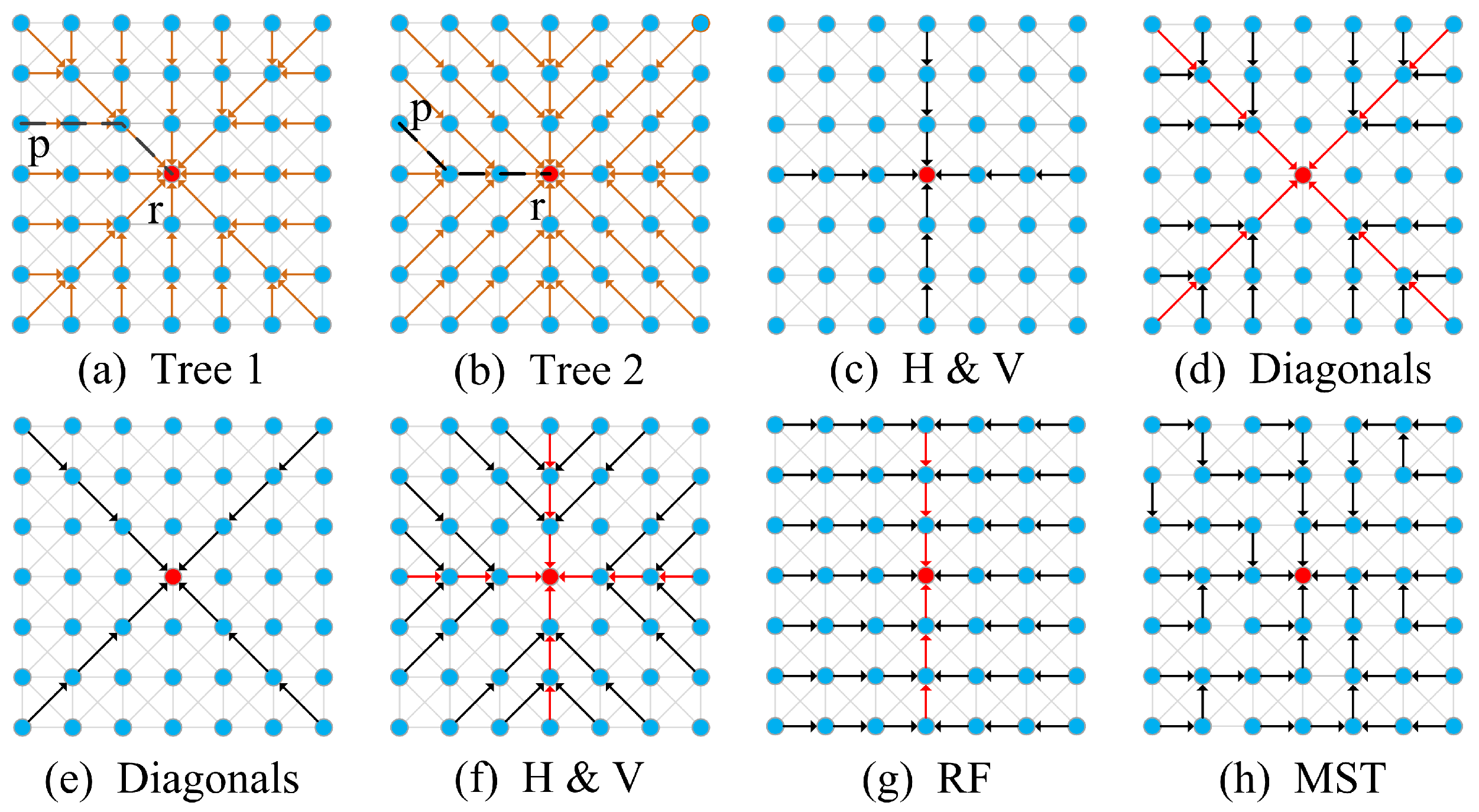
In this paper, we first propose an efficient non-local cost aggregation method that performs filtering along two complementary spatial tree structures, as shown in Figure 1a,b. The weight between any two pixels on each tree is the sum of the geodesic distances in both the spatial and intensity spaces and the final aggregated cost is the sum of the outputs from these two trees. The two spatial trees complement each other to balance the information propagated in all directions. The filtering procedure along each tree is implemented by aggregating costs along eight sub-trees. The eight sub-trees for Figure 1a are shown in (c) and (d), and they are (e) and (f) for Figure 1b. The filtering output on each sub-tree can be obtained by recursively aggregating costs from leaf nodes to the root node with linear time complexity. The only difference between performing cost aggregation along these two trees is filtering order. Experimental results in stereo matching and optical flow estimation validate the effectiveness of our method. Then, we compare handcrafted features and deep features extracted by CNNs in computing matching costs. In summary, our main contributions are:
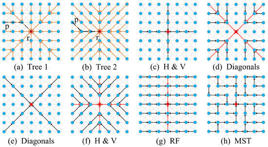
Figure 1.
Illustration of the filtering procedures along different tree structures. The black and red arrows indicate the directions of information propagated in the first and second steps, respectively. (a,b) show how the messages are propagated along our complementary spatial trees (Tree 1 and Tree 2) when calculating the output of the root node (the red node). The dot lines between nodes p and q indicate the different paths used to calculate the geodesic distances between pixels. (c,d) show the procedures to calculate the output of the root node on Tree 1. The filtering procedure is performed first along horizontal and vertical directions and then along diagonal directions. (e,f) show the procedure to calculate the output of the root node on Tree 2. The filtering procedure is performed first along diagonal, and then horizontal and vertical directions. (g) the filtering procedure of recursive filter [19]. The filtering procedure is performed in horizontal and vertical directions. (h) The way information propagated along the MST. See the text for details.
- Novel complementary spatial tree structures are proposed to perform non-local cost aggregation.
- Linear time complexity algorithms are presented to aggregate informative messages in all directions.
- A comparison of handcrafted features and deep features extracted by CNNs in computing matching costs.
- Experimental results in stereo matching and optical flow estimation show the effectiveness of our approach, which turns out our method outperforms typical MST-based non-local cost aggregation methods on the Middlebury [8] and KITTI [25,26] datasets.
The rest of this paper is organized as follows. We elaborate on our linear time non-local cost aggregation method based on two complementary spatial tree structures in Section 2. In Section 3, we provide the implementation and computational complexity of our algorithm. Experimental comparisons showing the superiority of our method are given in Section 4. Conclusion and future work are presented in Section 5.
2. Methods
The procedure of building initial cost volume for a rectified stereo pair can be formulated as , where H and W are the height and width of input images, 3 is the channels of a color image, and it is 1 for a gray input image. L is the disparity space, and we use to denote the matching cost of pixel at disparity l. Kinds of edge-aware filters have been designed to denoise the initial cost volume, aiming to enhance the quality of disparity images. Here, we elaborate on our non-local cost aggregation method which performs filtering along two complementary spatial tree structures with linear time complexity. The output of a pixel on each tree can be recursively computed from several sub-trees.
2.1. Cost Aggregation on Tree 1
Aggregating cost on Tree 1 can be implemented by filtering each cost slice in two steps: (1) Filtering each cost slice along horizontal and vertical directions to obtain the supports from pixels located in the same row and column, as shown in Figure 1c; (2) Filtering the outputs of the first step along diagonal tree structures to obtain supports from pixels on the sub-trees in diagonal directions, as shown in Figure 1d.
Step 1: The supports from pixels in the top, bottom, left, and right of root node can be obtained by filtering each cost slice along four directions, namely from top to bottom, bottom to top, left to right, and right to left. We let denote those four directions. The filtering output of pixel at disparity l in direction can be recursively computed by
where is the aggregated cost in direction , corresponding to the weight between root node and its previous pixel in direction .
Step 2: Other than the supports from pixels in vertical and horizontal directions, the supports from other pixels can be obtained by filtering the outputs of the first step along sub-trees in diagonal directions. Here, the four diagonal directions are denoted by , where , and we use and to represent the vectors in horizontal and vertical directions which satisfy . For instance, if , we have and . Therefore, the filtering output of pixel at disparity l in direction can be expressed as
where is the output of the sub-tree in direction . and are the filtering outputs in the first step for pixel at disparity l from the sub-trees in directions and , respectively.
Until now, for each pixel at disparity l, we have obtained the supports from pixels in the whole image, denoted by the filtering outputs along eight sub-trees in Tree 1, namely with , and with where . The aggregated cost of pixel at disparity l on Tree 1 is
where is the aggregated cost of pixel at disparity l on Tree 1. is subtracted in the formula so that is used four times in the computation of the outputs of sub-trees in horizontal and vertical directions.
In our approach, the reference image is divided into eight sub-trees, and the filtering outputs on these tree structures are fused to obtain the aggregated cost on Tree 1. As shown in Equations (1) and (2), we present a recursive strategy to compute the filtering output on each sub-tree. Thus, the computational complexity of our method on Tree 1 is time, where N is the resolution of the reference image.
2.2. Cost Aggregation on Tree 2
Performing cost aggregation on Tree 2 can also be implemented by filtering each cost slice in two steps: (1) filtering along diagonal directions to obtain the supports from pixels lying on these scanlines, as shown in Figure 1e; (2) filtering the outputs of the first step along sub-trees in vertical and horizontal directions, as shown in Figure 1f.
Step 1: Performance of filtering of each cost slice along scanlines in diagonal directions to obtain the supports from pixels on these scanlines. We denote the filtering output of the scanline in direction as . For pixel at disparity l, we have
The supports from other pixels on each scanline can be obtained by subtracting from the filtering output.
Step 2: The supports from pixels in non-diagonal directions can be obtained by filtering the outputs of the first step along sub-trees in vertical and horizontal directions, as shown in Figure 1f. We let and indicate the vectors in diagonal directions which satisfy . For instance, if , we have and . Thus, the filtering output of pixel at disparity l from the sub-tree in direction is
where is the support from pixels on the sub-tree in direction .
After performing cost aggregation along each sub-tree in Tree 2, we obtain eight outputs, namely with , and with where . Thus, the aggregated cost of pixel at disparity l on Tree 2 is
where is the aggregated cost on Tree 2. is subtracted in the formula so that is used four times in the computation of outputs of the sub-trees in four diagonal directions.
Although variables and appear in Equation (3) and Equation (6), they are quite different. in Equation (6) is the support from pixels on the scanline in direction , while it is the support from pixels on the sub-tree in this direction in Equation (3). in Equation (3) is only the support from pixels in horizontal or vertical directions, while it is the support from pixels on the sub-tree in the same direction in Equation (6).
The only difference between performing cost aggregation on Tree 1 and Tree 2 is the order of filtering procedures. Thus, our method has linear time complexity when performing cost aggregation on Tree 2.
2.3. Aggregated Cost on Complementary Spatial Trees
We perform cost aggregation on two complementary spatial tree structures to balance the supports from pixels in different directions, and the final aggregated cost for pixel at disparity l can be expressed as
We present a recursive strategy to compute the filtering result along each sub-tree, since only the weights among eight-connected neighborhoods are needed. We use both intensity similarity and spatial affinity to measure the distance between neighboring pixels. The distance in the range space is the maximum absolute difference between color vectors, and the spatial affinity is defined by the Euclidean distance. Thus, the weight between neighboring pixels u and v can be obtained by
where is the Euclidean distance between pixel u and pixel v; and correspond to the support ranges in both spatial and range spaces.
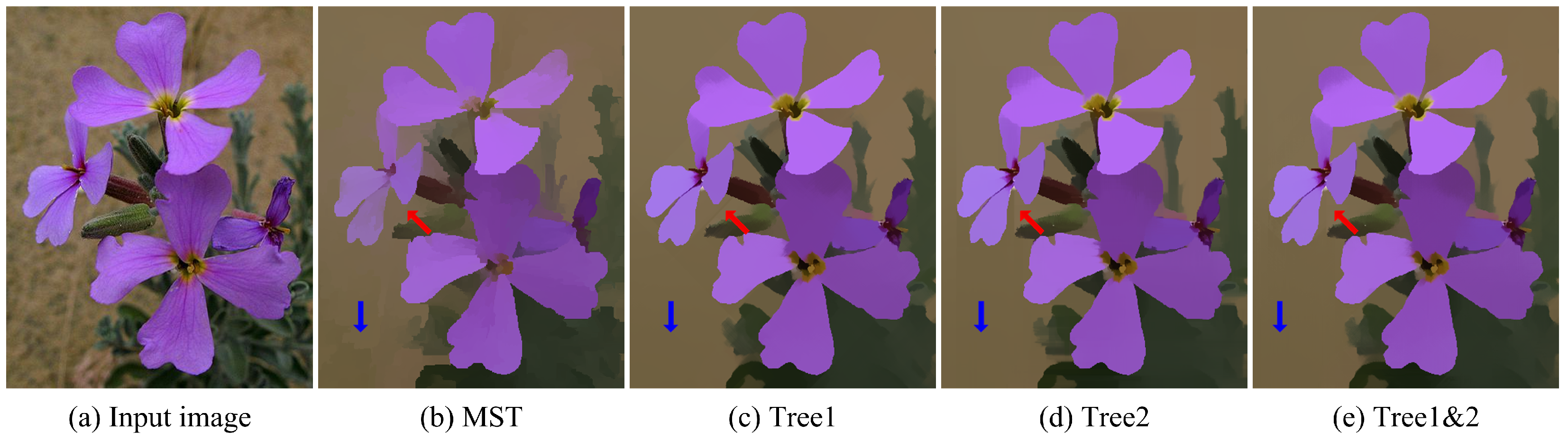
Table 1 presents a comparison of typical non-local filters. Both NL and ST need extra computation to build the tree structures, while DT and our method utilize the spatial relationship among pixels to propagate information across the entire image. All these non-local filters are implemented recursively to achieve high efficiency. The spatial distance between any two pixels for NL and ST is evaluated along the corresponding tree structure, while it is the Manhattan distance for DT. The spatial distance is composed of two parts in our method. They are along row/column and diagonal directions, as shown in Figure 1. Moreover, our method propagates information along the edges in the eight-connected neighborhood. NL, ST, and DT only utilize a section of edges in eight-connected neighbors. Figure 2 shows the results of filtering on different tree structures. It turns out that filtering along the MST tends to generate piece-wise constant results. The reason is that sub-trees in the MST are loosely connected since the informative message in each sub-tree has little impact on pixels in other sub-trees. Most pixels contribute to the output of the root node along diagonal directions on Tree 1, which are horizontal and vertical directions on Tree 2, resulting in stripe artifacts stretching along these two directions, denoted by red arrows in Figure 2c,d. We perform filtering along both Tree 1 and Tree 2 to balance the information propagated along all directions, which makes stripe artifacts visually unnoticeable.

Table 1.
Comparison of typical non-local filtering methods. Tree building: if extra computation is needed to build a tree structure. Implementation: the way to implement the filtering procedure. Spatial distance: the way to evaluate spatial distance between two pixels. Eight neighborhood: if messages propagate along eight directions.
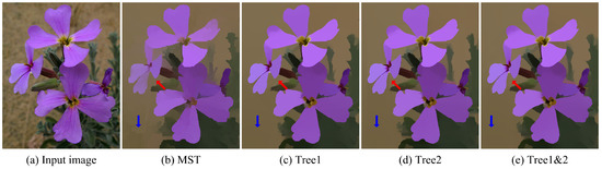
Figure 2.
Filtering results of different tree structures. (a) Input image. (b) Result of filtering along the MST. (c) Result of filtering along Tree 1. (d) Result of filtering along Tree 2. (e) Result of filtering along both Tree 1 and Tree 2. The blue arrows indicate the fake edges among sub-trees generated in the MST, and the red arrows indicate the streak artifacts when only filtering along one of our complementary spatial trees.
3. Implementation and Complexity
Our method performs cost aggregation along two complementary spatial trees, namely Tree 1 and Tree 2 in Figure 1a,b. The spatial distance and the intensity difference between pixels in the eight-connected neighborhood are computed first to obtain the weights in recursive filtering procedures. The cost aggregation on each tree is implemented by filtering along eight sub-trees, and the final aggregated cost of our approach is the sum of outputs from these two trees.
As the computational costs of performing cost aggregation on our two complementary spatial tree structures are the same, we elaborate on the computation required by performing cost aggregation on Tree 1, and the total computational cost of our method is twice that performing cost aggregation on Tree 1. From Equation (1), we can see that it needs four multiplication operations and four addition operations to obtain support from pixels located in the same row and column. Equation (2) needs four multiplication, four subtraction operations, and another eight addition operations to compute the support from pixels on sub-trees in diagonal directions. The fusion of the outputs from eight sub-trees in Equation (3) needs three subtraction and seven addition operations. Hence, seven subtraction, eight multiplication, and nineteen addition operations are required to calculate the aggregated cost of each pixel at each disparity level on Tree 1. As the computational complexities of performing cost aggregation on Tree 1 and Tree 2 are the same, our method has linear time complexity. Supposing the resolution of the reference image and the candidate disparity space are N and L, the computational cost of our approach is time.
Table 2 presents a running time comparison of typical edge-aware filtering approaches for one cost slice on a laptop with 2.0 GHz and 8 GB RAM. Both NL and ST extract tree structure from the reference image and recursively traverse the tree structure in two passes to aggregate informative messages across the whole image since they have the same computational complexity. The divergence of running time between NL and ST is due to different strategies adopted to implement the filtering procedure. GF needs to invert a three-by-three matrix when computing the filtering output for the color reference image. FCGF extends the support region of GF to the whole image to build complicated geometric structures of the input image. Although FCGF still has linear time complexity, the running time of FCGF is multiple times that of GF. Both spatial affinity and radiometric difference are utilized in BF to define the weights between neighboring pixels since the computational cost increases dramatically as the size of the support window rises.
Table 2.
Running time comparison of typical cost aggregation methods for each cost slice.
4. Results and Discussion
We perform experiments in optical flow estimation and stereo matching to demonstrate the effectiveness of our complementary spatial tree structures in cost aggregation. The ways of using our method in these two low-level vision tasks are almost identical, and the only difference is the strategy adopted to construct initial cost volume.
4.1. Stereo Matching
We use Middlebury and KITTI datasets to validate typical cost aggregation approaches, namely BF [12], GF [11], NL [16], DT [20], LRNL [28], FCGF [18], and ST [17]. The input stereo images are normalized to [0, 1] at first, and then used to compute matching costs at all candidate disparities. We use the implementations in cross-scale cost aggregation [10] for BF, GF, NL, and ST, and implement FCGF by referring to the elaboration in paper [18]. Default parameters are used in these approaches to generate satisfactory results. We use 0.05 for and 10 for on the Middlebury dataset and halve them on the KITTI dataset, as there is a large portion of textureless regions in the KITTI dataset.
4.1.1. Middlebury Dataset
The Middlebury dataset contains kinds of indoor artificial scenes taken under a controlled environment with pixel-level accuracy ground truth generated by structured light. We adopt pixel-based truncated absolute differences of both color vector and gradient to measure the proximity of matching pixels. Thus, the initial matching cost of pixel at disparity l can be computed by
where and are the color vectors of two candidate matching pixels and in the left and right images, is the gradient operation in the x direction. balances the gradient and color terms. , and correspond to the truncation values of these two terms. In our experiments, , , and are 0.89, 7/255, and 2/255, respectively. Both left and right images are used as guidance images to generate corresponding disparity images. We use the left–right consistency check to classify pixels into stable and unstable, and the non-local refinement method [16] is adopted to propagate reliable disparities from stable pixels to unstable ones.
Table 3 lists the error rate of non-occluded and all regions for typical cost aggregation methods. Our method outperforms BF, LRNL, FCGF, NL, DT, and ST at all metrics. NL, ST, and FCGF are all tree-based non-local filters. ST enforces tight connections for pixels in a neighborhood by building pixel-level and region-level tree structures so that the over-smoothing problem of NL can be alleviated, leading to better results. FCGF reduces the supports of neighboring pixels and generates noisy disparity images. DT can only propagate informative messages along the horizontal or vertical direction in each pass since it produces the worst results among these approaches. Both BF and GF take advantage of local structures to evaluate the similarity of neighboring pixels. However, GF adopts a linear model aiming to preserve the structure of the guidance image so that it produces more satisfactory results. We perform cost aggregation on two spatial trees, which balances the information propagated along all directions. After post-processing, our method generates competitive or even better results than GF. Moreover, our approach is more efficient than GF, as shown in Table 2.
Table 3.
Quantitative comparison with typical cost aggregation approaches on the Middlebury dataset [8]. Out_a and Out_n are the percentages of erroneous pixels in all and non-occluded regions, respectively (/%). The bold is the best result in each metric.
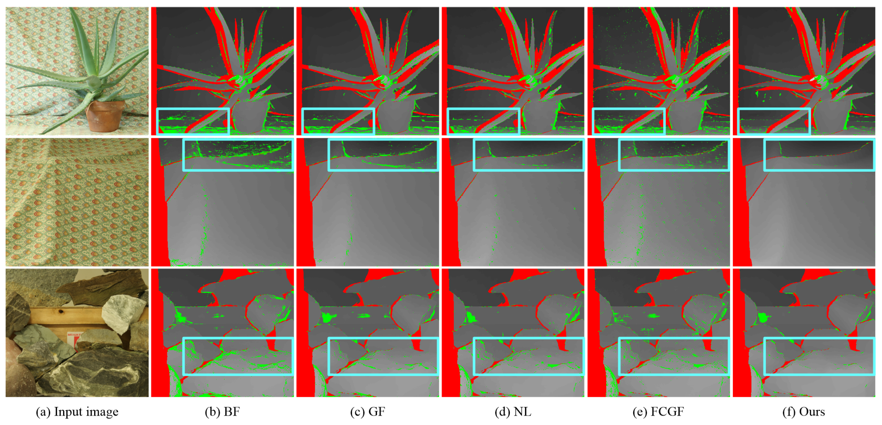
Figure 3 presents the final disparity images of typical cost aggregation methods. All these approaches can correctly estimate the disparities of pixels in highly textured regions. BF and GF assume all pixels in the support window on a disparity plane. NL and FCGF utilize the MST of the input image to build long-range connections. However, they tend to overuse the piece-wise constant assumption. Thus, BF, GF, NL, and FCGF produce many erroneous disparities in slant surfaces, as indicated by the boxes in the first row of Figure 3b–e. Compared with BF and GF, NL and FCGF weaken the constraints from neighboring pixels. Hence, NL and FCGF produce better results in regions containing fine-scale details, as indicated by the boxes in the second row in Figure 3b–e. Our method overcomes these shortages by recursive filtering and balancing the information propagated in all directions. Thus, our approach can successfully preserve fine-scale details in highly textured regions and alleviate the over-smoothing problem in slant surfaces, as shown in Figure 3f.
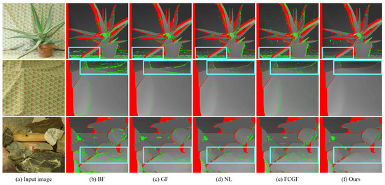
Figure 3.
Results of typical cost aggregation methods on the Middlebury dataset [8]. Mismatched pixels in occluded and non-occluded regions are indicated by red and green, respectively. (a) Input image. (b) Bilateral filter [29]. (c) Guided filter [13]. (d) Non-local filter [16]. (e) Fully connected guided filter [18]. (f) Our method.
4.1.2. KITTI Dataset
Both KITTI 2012 [25] and KITTI 2015 [26] datasets are real-world street views of both highways and rural areas captured by a driving car under natural conditions since there is a large portion of textureless regions in these stereo pairs. We adopt both the Census Transform and the correlation of deep features extracted by CNNs to compute matching costs and then evaluate the performance of these two cost functions under different cost aggregation methods. The main idea of Census Transform is to use a string of bits to characterize the pixels in the local window. We suppose the size of the local window is ; thus, the Census Transform of pixel can be defined as
where is the string of bits for pixel after Census Transform and ⊗ is the bit-wise concatenation operation. The Hamming distance of two strings of bits is utilized to measure the similarity of pixels. The matching cost of pixel at disparity l is
where and are the two strings of bits for matching pixels in the left and right images, is the operation to calculate Hamming distance, and indicates the matching cost of the handcrafted feature. As for features extracted by CNNs, we directly use the correlation of left and right features to evaluate the similarity of matching pixels. The PSMNet [24] combines spatial pyramid pooling and dilated convolution to enlarge the receptive field. The resultant local and global features aggregate context information at different scales and locations and are widely used in many state-of-the-art methods [23,30,31]. We also use the PSMNet to extract deep features in our experiments. We denote the learned features as , so the matching cost of pixel at disparity l can be expressed as
where is the matching cost of features extracted by CNNs, and represent the deep features of left and right images, is the norm. Typical cost aggregation methods are utilized to improve the robustness of matching costs. In the refinement step, the left–right consistency check is used to identify mismatched pixels, and those mismatched pixels are assigned to the lowest disparity value of the spatially closest matched pixels on the same scanline. Finally, we adopt the weighted median filter to remove streak artifacts. The error threshold in our evaluation is 3.
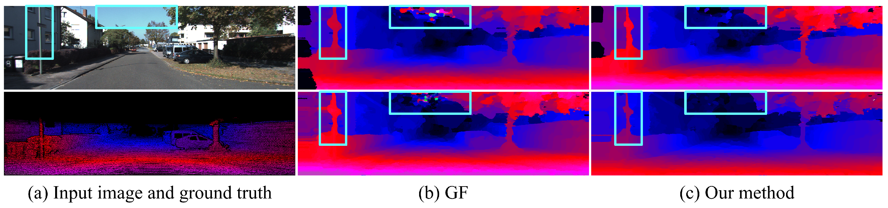
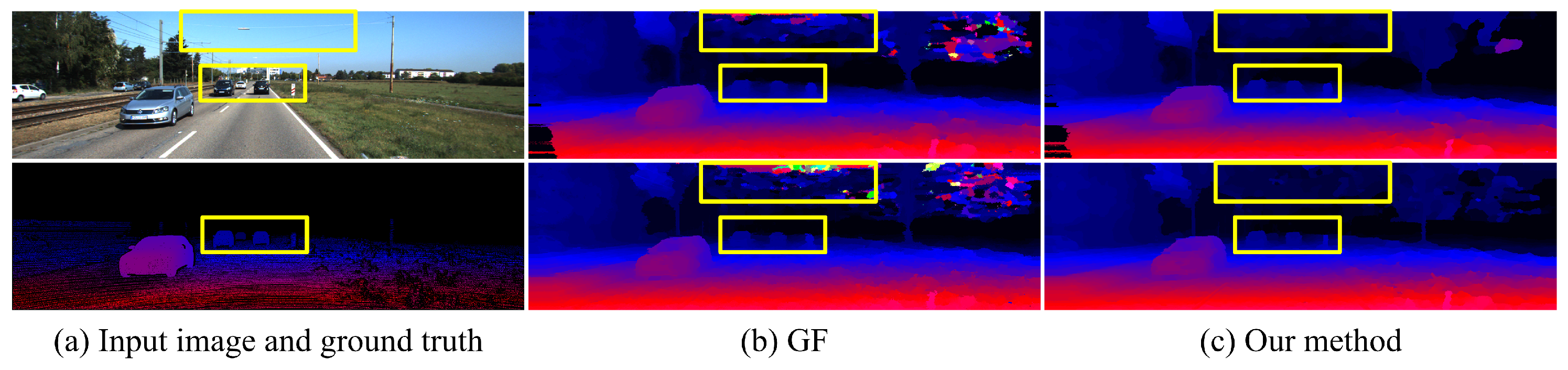
Qualitative evaluation: Figure 4 and Figure 5 present a comparison of GF and our method using two kinds of features to compute the matching costs on the KITTI 2012 and KITTI 2015 datasets. GF can effectively filter out noise in textured regions by taking advantage of local structure in the guidance image but fails to preserve fine-scale details in real-world stereo pairs. The reason is that the intensity difference between foreground and background is indistinctive in many cases since the local linear regression model used in GF cannot accurately distinguish fine-scale details from background. Moreover, GF fails to filter out the noise in large homogeneous regions, such as the sky. Due to this, there is no informative message in these areas, resulting in matching costs at different candidate disparities becoming identical. Our method performs non-local coat aggregation on two complementary spatial tree structures, and the geodesic distances in both spatial and intensity spaces are used to evaluate the similarity of pixels along these two trees. Therefore, our method propagates informative messages across the entire image to deal with challenging occasions, for example, the degradation of region-based cost function for fine-scale structures and the lack of useful information in homogeneous areas.

Figure 4.
Comparison of disparity images using deep features from PSMNet [24] (top row) and handcrafted feature (second row) to compute matching cost on the KITTI 2012 dataset. (a) Guidance image and sparse ground-truth disparity image. (b) Guided Filter [11]. (c) Our method.
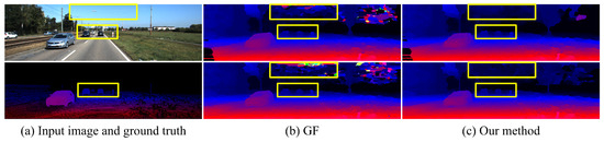
Figure 5.
Comparison of disparity images using deep features from PSMNet [24] (top row) and handcrafted feature (second row) to compute matching cost on the KITTI 2015 dataset. (a) Guidance image and sparse ground-truth disparity image. (b) Guided Filter [11]. (c) Our method.
The results of each method using different features to compute matching cost demonstrate that handcrafted features tend to generate more edge-aware disparity images while deep features produce better results in textureless regions. The reason is that deep CNNs with a large receptive field can utilize textural information from a wide range, improving the robustness of deep features for pixels in homogeneous areas.
Quantitative evaluation: Table 4 presents the error rate and average end-point error of typical cost aggregation methods on the KITTI 2012 dataset. Our approach surpasses NL, ST, and FCGF in all metrics. Although the error rates of both initial and final disparity images are smaller than ours, the average end-point error of our method is close to or even smaller than that of GF. The main reason for this phenomenon is that only the disparities of pixels near the ground are provided in ground-truth disparity images. Most of those valid pixels are located in highly textured regions so that GF can utilize the structure information in the local area to generate high-quality results. Our method is superior to GF in homogeneous regions, as shown in Figure 4 and Figure 5. HASR incorporates edge information with CT to further compensate for radiometric changes and adopts a hierarchical cross-based cost aggregation scheme to fuse costs at multiple scales. These strategies make their method obtain the lowest error rate in non-occluded regions. However, the end-point errors in non-occluded and all areas are 1.9 px and 2.9 px, which are 0.3 px and 1.02 px larger than ours. The reason is that they incorporate multi-scale costs by an exponential function while we take advantage of the inter-scale regularization [10].
Table 4.
Quantitative comparison of typical cost aggregation approaches using handcrafted features to compute matching cost on the KITTI 2012 dataset [25]. Avg_n and Avg_a are the end-point errors in non-occluded and all regions, respectively (/px). “/”: the results are not available. The bold is the best result in each metric.
Table 5 lists the results of GF, NL, FCGF, ST, LRNL, and our method using deep features extracted by PSMNet [24] to compute the matching cost. Compared with the results generated by the handcrafted feature of GF, FCGF, NL, and ST, the average error rate and end-point error of these cost aggregation methods in non-occluded regions decreased from 12.54% and 2.50 px to 9.27% and 2.32 px, improved by 26.08% and 7.20%, respectively. The average error rates of final disparity images are still lower than that of the handcrafted feature. The reason is that CNNs can incorporate information in a large receptive field to improve the robustness of features in textureless areas. Our method outperforms LRNL in all metrics by a margin. It turns out that keeping the information propagated along all directions in balance is vital for improving the quality of disparity images. Figure 6 presents examples of disparity images and corresponding error maps of our method using the handcrafted feature and deep ones to compute the matching cost. Our approach correctly estimates the disparities of most pixels in the guidance image. Pixels with significant errors are mainly located at occluded regions as they have no matching pixels in the other view. Comparing the error maps of these two kinds of features, the average end-point error of pixels in occluded areas of handcrafted features is smaller than that of deep ones. The reason is that the matching costs of handcrafted features are less distinctive than those of deep features since it is easier to propagate reliable information from non-occlusion regions to occluded areas.
Table 5.
Quantitative comparison of typical cost aggregation approaches on the KITTI 2012 dataset [25] using deep features extracted by PSMNet [24] to compute the matching cost. The bold is the best result in each metric.
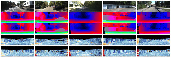
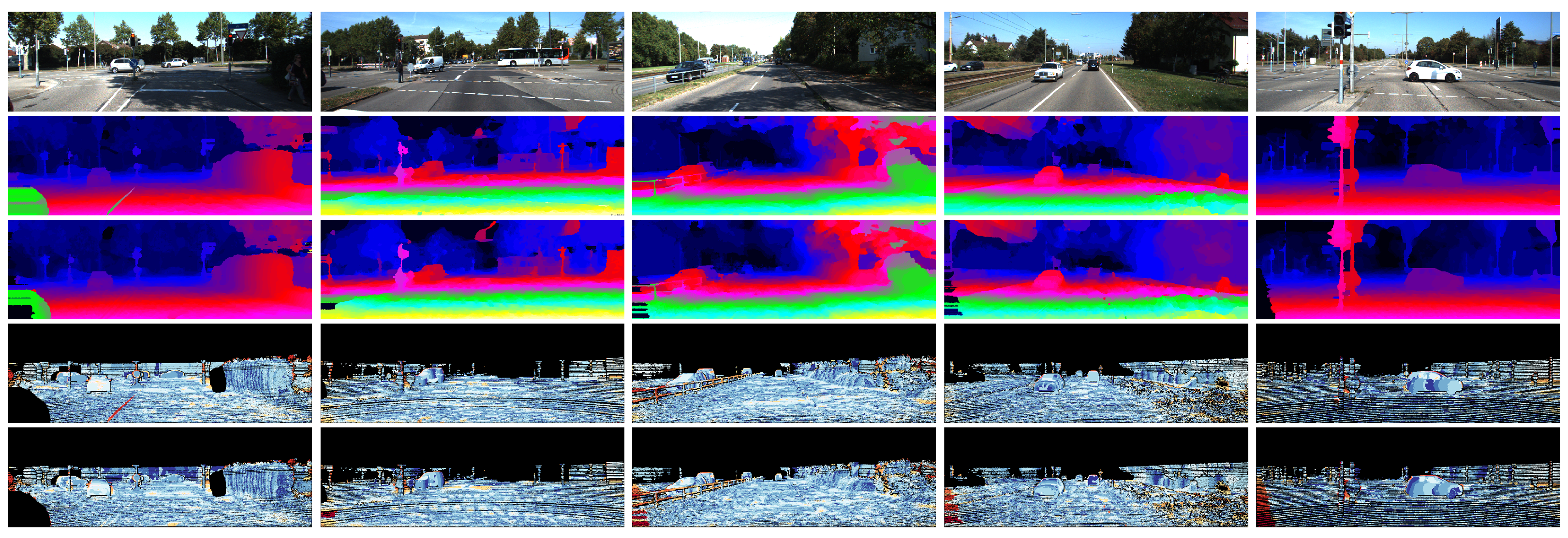
Figure 6.
Disparity images and corresponding error maps of our approach using the handcrafted feature and deep features to compute the matching costs on the KITTI 2012 dataset [25]. From top to bottom: Input reference image, disparity image using the handcrafted feature, disparity image using deep ones extracted by PSMNet [24], error map of disparity image using the handcrafted feature, error map of disparity image using deep features extracted by PSMNet [24].
Table 6 presents the results of different approaches using the handcrafted feature to compute the matching cost on the KITTI 2015 dataset [26]. Our method achieves the best results in most metrics. Compared with FCGF, the average end-point errors of the initial disparity images in all and non-occluded regions are decreased by 0.63 px and 0.66 px, and the error rates in these regions are reduced by about 4.3% and 4.4%, respectively. Although the error rates of GF are lower than ours after refinement, we achieve the lowest average end-point error among these methods. It means that the end-point error of most outliers of our approach is smaller than that of GF. Table 7 lists the results of typical methods on the KITTI 2015 dataset using deep features extracted by PSMNet [24] to compute the matching cost. Our approach surpasses all other methods in all metrics. Comparing our statistics with those of other non-local cost aggregation methods on both KITTI 2012 [25] and KITTI 2015 [26], our method achieves the best performance. Thus, we can conclude that the geodesic distance depending on the relative spatial relationship could be better than considering the similarity of pixels on an MST or its variants. The reason could be that geodesic distance can help to weaken the piece-wise constant assumption, leading to more accurate disparities in regions composed of large slant planes, such as roads.
Table 6.
Quantitative comparison of different approaches on the KITTI 2015 dataset [26] using the handcrafted feature to compute the matching cost. The bold is the best result in each metric.
Table 7.
Quantitative comparison of typical cost aggregation approaches on the KITTI 2015 dataset [26] using the deep features extracted by PSMNet [24] to compute the matching cost. The bold is the best result in each metric.
Figure 7 shows disparity images and corresponding error maps of our method using both the handcrafted feature and the deep features to compute the matching cost on the KITTI 2015 dataset [26]. We can see that the matching costs generated by deep features can deal with radiometric variations in real-world images. However, it suffers from propagating useful information to occluded areas in the image border, resulting in a higher average end-point error.
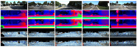
Figure 7.
Disparity images and corresponding error maps of our approach using the handcrafted and deep ones to compute the matching costs on the KITTI 2015 dataset [26].
4.2. Optical Flow Estimation
Optical flow estimation aims to estimate the change in spatial location of objects with respect to time from image sequences. Supposing label l corresponding to vector denotes the motion in the x and y directions, the matching cost of pixel at label l can be computed by
where is the gradient in the y direction. The other variables are the same as that in stereo matching, and the values of parameters , , and remain the same. We use left and right images as the guidance images to derive the initial flow fields and adopt the same strategies as stereo matching to refine them. To generate flow maps with sub-pixel accuracy, we use bicubic interpolation to upscale input images, which only leads to an increase in the label space. In practice, we use an upscaling parameter of four and compare our results with that of GF, which has been proven to outperform many cost aggregation methods in optical flow estimation.
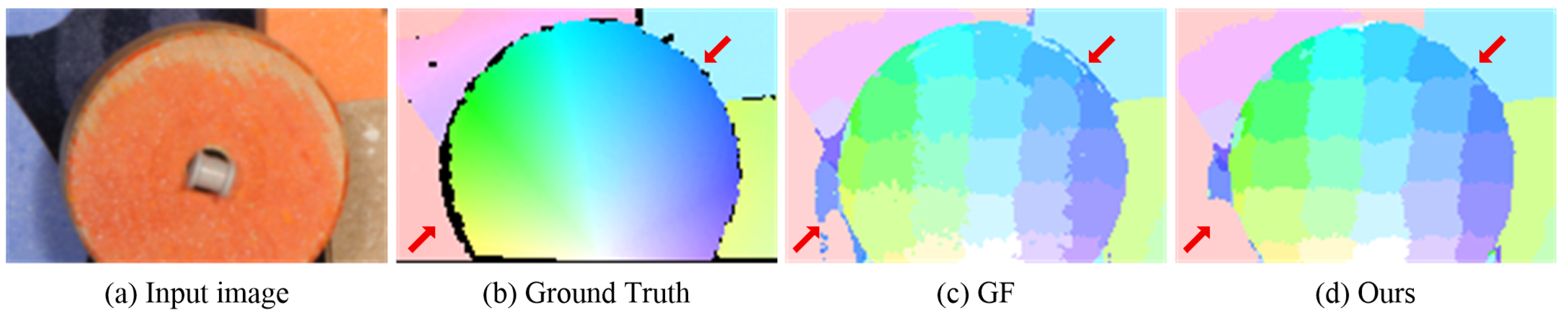
Figure 8 presents the initial flow maps of GF and our method with pixel-level accuracy on the Middlebury flow dataset [35]. These two methods can correctly estimate the motion of the main structures in the input image. The non-local property of our approach alleviates the ambiguity in homogeneous and occluded regions by encouraging informative messages to propagate in a wide range, as marked by the arrow in the bottom left. Another advantage is that our method can correctly preserve the discontinuities in flow maps where foreground and background are similar, as marked by the arrow in the top right.
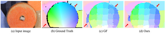
Figure 8.
Comparison of the initial flow maps for RubberWhale generated by GF [13] and our method. (a) Input image. (b) Ground-truth flow map. (c) Initial flow maps of GF. (d) Initial flow maps of our method. The red arrows show that our method generates better results.
We quantitatively compare our method with GF on Dimetrodon, Grove2, and RubberWhale images with ground truth provided by Baker et al. [35]. The end-point error (EDE) and average angular error (AE) are adopted to evaluate the performance of these two methods. Table 8 presents the initial and final flow maps. Figure 9 shows examples of flow maps and close-ups with sub-pixel accuracy. Our method outperforms GF on RubberWhale as it contains large textureless regions with unreliable matching costs. GF only utilizes matching costs over a local support window and fails to solve the ambiguity in these regions. GF obtains lower errors in both initial and final flow maps on Groves2. The reason is that our strategy attempts to approximate the geodesic distances in both spatial and intensity spaces. Thus, reliable information cannot propagate in a long range under these circumstances, leading to erroneous flow, as shown in the close-ups in Figure 9. However, this can be amended by reducing in Equation (8). Moreover, our method is more efficient than GF.
Table 8.
Quantitative comparison of cost aggregation on flow estimation. AE ± std: Average agular error. EDE: Endpoint error (px).
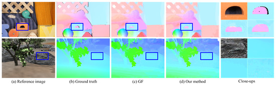
Figure 9.
Qualitative comparison of GF and our method in optical flow estimation. (a) Input image. (b) Ground-truth flow map. (c) Guided filter [13]. (d) Our method.
5. Conclusions and Future Work
In this paper, we propose an efficient non-local cost aggregation method on two complementary spatial tree structures. Recursive algorithms with linear time complexity are presented to compute the output on each tree. Our spatial tree structures provide more suitable ways to calculate the geodesic distances in spatial and intensity spaces. The integration of these two trees balances the information propagated in all directions. Experimental results in stereo matching and optical flow estimation demonstrate that our method is superior to MST-based non-local filtering methods. We also compare handcrafted features and deep features extracted by CNNs in stereo matching. The results show that handcrafted features can successfully preserve the discontinuities in disparity images, while deep features extracted by CNNs are superior at dealing with ambiguity in homogeneous regions. After refinement, the percentage of erroneous pixels and average end-point error in non-occluded areas using features extracted by deep CNNs to compute matching costs are improved by 37.2% and 8.2%, respectively. It is straightforward to fuse the matching costs of these two kinds of features based on the texture pattern in the local area. Moreover, our method can also be applied to edge-preserving graphics applications. We will work on this in the future.
Author Contributions
Conceptualization, H.W. and H.Z.; methodology, P.B.; software, P.B.; validation, P.B. and H.Z.; investigation, Y.D.; resources, Y.D.; writing—original draft preparation, P.B.; writing—review and editing, P.B.; visualization, P.B.; supervision, Y.D.; project administration, H.Z.; funding acquisition, P.B. and H.Z. All authors have read and agreed to the published version of the manuscript.
Funding
This research was funded by the Research and Development Program of Shaanxi Province (Grant no. 2023-YBGY-103) and the National Natural Science Foundation of China (Grant No. 61975161).
Institutional Review Board Statement
Not applicable.
Informed Consent Statement
Not applicable.
Data Availability Statement
The data presented in this study are openly available in https://www.cvlibs.net/datasets/kitti/eval_stereo.php and https://vision.middlebury.edu/stereo/data/, accessed on 15 March 2017.
Acknowledgments
The authors would like to thank Tao Yang for his help in applying the Research and Development Program of Shaanxi Province (Grant no. 2023-YBGY-103) and preparing this manuscript. We appreciate the help from anonymous editors and reviewers for their valuable suggestions.
Conflicts of Interest
The authors declare no conflict of interest.
Abbreviations
The following abbreviations are used in this manuscript:
| BF | Bilateral filter |
| GF | Guided filter |
| NL | Non-local filter |
| ST | Segment-tree filter |
| DT | Domain Transform |
| FCGF | Fully connected guided filter |
| LRNL | Linear recursive non-local filter |
References
- Zeglazi, O.; Rziza, M.; Amine, A.; Demonceaux, C. A hierarchical stereo matching algorithm based on adaptive support region aggregation method. Pattern Recognit. Lett. 2018, 112, 205–211. [Google Scholar] [CrossRef]
- Yao, Y.; Luo, Z.; Li, S.; Fang, T.; Quan, L. Mvsnet: Depth inference for unstructured multi-view stereo. In Proceedings of the European Conference on Computer Vision (ECCV), Munich, Germany, 8–14 September 2018; pp. 767–783. [Google Scholar]
- Shrivastava, A.; Malisiewicz, T.; Gupta, A.; Efros, A.A. Data-driven visual similarity for cross-domain image matching. ACM Trans. Graph. 2011, 30, 154. [Google Scholar] [CrossRef]
- Truong, P.; Apostolopoulos, S.; Mosinska, A.; Stucky, S.; Ciller, C.; Zanet, S.D. Glampoints: Greedily learned accurate match points. In Proceedings of the IEEE/CVF International Conference on Computer Vision, Seoul, Republic of Korea, 27 October–2 November 2019; pp. 10732–10741. [Google Scholar]
- Sun, X.; Chen, C.; Wang, X.; Dong, J.; Zhou, H.; Chen, S. Gaussian dynamic convolution for efficient single-image segmentation. IEEE Trans. Circuits Syst. Video Technol. 2021, 32, 2937–2948. [Google Scholar] [CrossRef]
- Lv, X.; Wang, X.; Wang, Q.; Yu, J. 4D light field segmentation from light field super-pixel hypergraph representation. IEEE Trans. Vis. Comput. Graph. 2020, 27, 3597–3610. [Google Scholar] [CrossRef] [PubMed]
- Lu, Y.; Sarkis, M.; Lu, G. Multi-task learning for single image depth estimation and segmentation based on unsupervised network. In Proceedings of the 2020 IEEE International Conference on Robotics and Automation (ICRA), Paris, France, 31 May–31 August 2020; pp. 10788–10794. [Google Scholar]
- Scharstein, D.; Szeliski, R. A taxonomy and evaluation of dense two-frame stereo correspondence algorithms. Int. J. Comput. Vis. 2002, 47, 7–42. [Google Scholar] [CrossRef]
- Hirschmuller, H.; Scharstein, D. Evaluation of stereo matching costs on images with radiometric differences. IEEE Trans. Pattern Anal. Mach. Intell. 2008, 31, 1582–1599. [Google Scholar] [CrossRef]
- Zhang, K.; Fang, Y.; Min, D.; Sun, L.; Yang, S.; Yan, S.; Tian, Q. Cross-scale cost aggregation for stereo matching. In Proceedings of the IEEE Conference on Computer Vision and Pattern Recognition, Columbus, OH, USA, 23–28 June 2014; pp. 1590–1597. [Google Scholar]
- Hosni, A.; Rhemann, C.; Bleyer, M.; Rother, C.; Gelautz, M. Fast cost-volume filtering for visual correspondence and beyond. IEEE Trans. Pattern Anal. Mach. Intell. 2012, 35, 504–511. [Google Scholar] [CrossRef]
- Yoon, K.J.; Kweon, I.S. Adaptive support-weight approach for correspondence search. IEEE Trans. Pattern Anal. Mach. Intell. 2006, 28, 650–656. [Google Scholar] [CrossRef] [PubMed]
- He, K.; Sun, J.; Tang, X. Guided image filtering. IEEE Trans. Pattern Anal. Mach. Intell. 2012, 35, 1397–1409. [Google Scholar] [CrossRef]
- Hosni, A.; Bleyer, M.; Gelautz, M.; Rhemann, C. Local stereo matching using geodesic support weights. In Proceedings of the 2009 16th IEEE International Conference on Image Processing (ICIP), Cairo, Egypt, 7–10 November 2009; pp. 2093–2096. [Google Scholar]
- Zhang, K.; Lu, J.; Lafruit, G. Cross-based local stereo matching using orthogonal integral images. IEEE Trans. Circuits Syst. Video Technol. 2009, 19, 1073–1079. [Google Scholar] [CrossRef]
- Yang, Q. A non-local cost aggregation method for stereo matching. In Proceedings of the 2012 IEEE Conference on Computer Vision and Pattern Recognition, Providence, RI, USA, 16–21 June 2012; pp. 1402–1409. [Google Scholar]
- Mei, X.; Sun, X.; Dong, W.; Wang, H.; Zhang, X. Segment-tree based cost aggregation for stereo matching. In Proceedings of the IEEE Conference on Computer Vision and Pattern Recognition, Portland, OR, USA, 23–28 June 2013; pp. 313–320. [Google Scholar]
- Dai, L.; Yuan, M.; Zhang, F.; Zhang, X. Fully connected guided image filtering. In Proceedings of the IEEE International Conference on Computer Vision, Santiago, Chile, 11–13 December 2015; pp. 352–360. [Google Scholar]
- Gastal, E.S.; Oliveira, M.M. Domain transform for edge-aware image and video processing. In ACM SIGGRAPH 2011 Papers; ACM: New York, NY, USA, 2011; pp. 1–12. [Google Scholar]
- Pham, C.C.; Jeon, J.W. Domain transformation-based efficient cost aggregation for local stereo matching. IEEE Trans. Circuits Syst. Video Technol. 2012, 23, 1119–1130. [Google Scholar] [CrossRef]
- Kendall, A.; Martirosyan, H.; Dasgupta, S.; Henry, P.; Kennedy, R.; Bachrach, A.; Bry, A. End-to-end learning of geometry and context for deep stereo regression. In Proceedings of the IEEE International Conference on Computer Vision, Venice, Italy, 22–29 October 2017; pp. 66–75. [Google Scholar]
- Tulyakov, S.; Ivanov, A.; Fleuret, F. Weakly supervised learning of deep metrics for stereo reconstruction. In Proceedings of the IEEE International Conference on Computer Vision, Venice, Italy, 22–29 October 2017; pp. 1339–1348. [Google Scholar]
- Zhang, Y.; Chen, Y.; Bai, X.; Yu, S.; Yu, K.; Li, Z.; Yang, K. Adaptive Unimodal Cost Volume Filtering for Deep Stereo Matching. In Proceedings of the AAAI, New York, NY, USA, 7–12 February 2020; pp. 12926–12934. [Google Scholar]
- Chang, J.R.; Chen, Y.S. Pyramid stereo matching network. In Proceedings of the IEEE Conference on Computer Vision and Pattern Recognition, Salt Lake City, UT, USA, 18–23 June 2018; pp. 5410–5418. [Google Scholar]
- Geiger, A.; Lenz, P.; Urtasun, R. Are we ready for autonomous driving? The kitti vision benchmark suite. In Proceedings of the 2012 IEEE Conference on Computer Vision and Pattern Recognition, Providence, RI, USA, 16–21 June 2012; pp. 3354–3361. [Google Scholar]
- Menze, M.; Geiger, A. Object scene flow for autonomous vehicles. In Proceedings of the IEEE Conference on Computer Vision and Pattern Recognition, Boston, MA, USA, 7–12 June 2015; pp. 3061–3070. [Google Scholar]
- Yang, Q. Stereo matching using tree filtering. IEEE Trans. Pattern Anal. Mach. Intell. 2014, 37, 834–846. [Google Scholar] [CrossRef] [PubMed]
- Bu, P.; Zhao, H.; Jin, Y.; Ma, Y. Linear Recursive Non-Local Edge-Aware Filter. IEEE Trans. Circuits Syst. Video Technol. 2020, 31, 1751–1763. [Google Scholar] [CrossRef]
- Tomasi, C.; Manduchi, R. Bilateral filtering for gray and color images. In Proceedings of the Sixth International Conference on Computer Vision (IEEE Cat. No. 98CH36271), Bombay, India, 4–7 January 1998; pp. 839–846. [Google Scholar]
- Guo, X.; Yang, K.; Yang, W.; Wang, X.; Li, H. Group-wise correlation stereo network. In Proceedings of the IEEE/CVF Conference on Computer Vision and Pattern Recognition, Long Beach, CA, USA, 15–20 June 2019; pp. 3273–3282. [Google Scholar]
- Song, X.; Yang, G.; Zhu, X.; Zhou, H.; Wang, Z.; Shi, J. Adastereo: A simple and efficient approach for adaptive stereo matching. In Proceedings of the IEEE/CVF Conference on Computer Vision and Pattern Recognition, Nashville, TN, USA, 20–25 June 2021; pp. 10328–10337. [Google Scholar]
- Oguri, K.; Shibata, Y. A new stereo formulation not using pixel and disparity models. arXiv 2018, arXiv:1803.01516. [Google Scholar]
- Zeglazi, O.; Rziza, M.; Amine, A.; Demonceaux, C. Accurate dense stereo matching for road scenes. In Proceedings of the 2017 IEEE International Conference on Image Processing (ICIP), Beijing, China, 17–20 September 2017; pp. 720–724. [Google Scholar]
- Hamzah, R.A.; Ibrahim, H.; Hassan, A.H.A. Stereo matching algorithm based on per pixel difference adjustment, iterative guided filter and graph segmentation. J. Vis. Commun. Image Represent. 2017, 42, 145–160. [Google Scholar] [CrossRef]
- Baker, S.; Scharstein, D.; Lewis, J.; Roth, S.; Black, M.J.; Szeliski, R. A database and evaluation methodology for optical flow. Int. J. Comput. Vis. 2011, 92, 1–31. [Google Scholar] [CrossRef]


Disclaimer/Publisher’s Note: The statements, opinions and data contained in all publications are solely those of the individual author(s) and contributor(s) and not of MDPI and/or the editor(s). MDPI and/or the editor(s) disclaim responsibility for any injury to people or property resulting from any ideas, methods, instructions or products referred to in the content. |
© 2023 by the authors. Licensee MDPI, Basel, Switzerland. This article is an open access article distributed under the terms and conditions of the Creative Commons Attribution (CC BY) license (https://creativecommons.org/licenses/by/4.0/).