Abstract
Student dropout is a serious issue in that it not only affects the individual students who drop out but also has negative impacts on the former university, family, and society together. To resolve this, various attempts have been made to predict student dropout using machine learning. This paper presents a model to predict student dropout at Sahmyook University using machine learning. Academic records collected from 20,050 students of the university were analyzed and used for learning. Various machine learning algorithms were used to implement the model, including Logistic Regression, Decision Tree, Random Forest, Support Vector Machine, Deep Neural Network, and LightGBM (Light Gradient Boosting Machine), and their performances were compared through experiments. We also discuss the influence of oversampling used to resolve data imbalance issues in the dropout data. For this purpose, various oversampling algorithms such as SMOTE, ADASYN, and Borderline-SMOTE were tested. Our experimental results showed that the proposed model implemented using LightGBM provided the best performance with an F1-score of 0.840, which is higher than the results of previous studies discussing the dropout prediction with the issue of class imbalance.
1. Introduction
Student dropout has been recognized as the most complex and important issue in education systems [1]. It has a negative impact not only on individual students but also on society [2]. From the perspective of individual students, this results in failing to obtain a degree, which may limit opportunities for securing quality employment and lower income. Re-admission or transferring to another university could entail additional time and financial loss. From the perspective of society, it can be a factor that increases social security costs, such as re-employment training costs and unemployment benefits, since students who drop out may need additional employment training or remain unemployed due to a lack of skills. Also, from the perspective of universities, student dropout leads to direct financial losses and has a negative impact on financial operations due to increased expenses arising from the selection of additional students.
Machine learning has been used effectively in a variety of research fields [3,4], and it has also been employed in the majority of existing studies to predict whether or not students will drop out [5,6,7]. Dropout prediction can be modeled as a binary classification problem, and its performance can be influenced by the dropout rate of the source data used for learning. The problem is that the dropout rate is either quite high or low depending on the university or educational institution. For example, as of 2018, the dropout rate of 4-year universities in South Korea is approximately 5% [8,9], while the rate increases to 18.9% for cyber universities [10]. On the other hand, the dropout rate of online open lecture systems, including Massive Open Online Courses (MOOCs), is extremely high, up to 80–95% [11,12,13]. From this, the prediction accuracy can be significantly influenced by the data imbalance caused by the extremely high or low dropout rate. In order to achieve high accuracy, it is essential to reflect such imbalance properly in learning. It is also necessary to adopt performance indicators that account for the data imbalance when evaluating the performance of prediction models.
This paper presents a model to predict student dropout at Sahmyook University, a small- and medium-sized 4-year university located in Seoul. About 168,000 academic records collected from 20,050 students from 2010 to 2022 were analyzed and used for learning. Various machine learning algorithms were used to implement the model, including Logistic Regression (LR) [14], Decision Tree (DT) [15], Random Forest (RF) [16], Support Vector Machine (SVM) [17], Deep Neural Network (DNN) [18], and Light Gradient Boosting Machine (LightGBM) [19], and their performance were compared through experiments. In addition, we discuss the influence of oversampling used to resolve the data imbalance mentioned above. For this purpose, various oversampling techniques, such as SMOTE [20], ADASYN [21], and Borderline-SMOTE [22], were tested. To compare the performance of models, the F1-score was used, which is a performance metric that properly reflects the data imbalance in the performance evaluation.
This paper is organized as follows. Section 2 introduces existing studies related to dropout prediction using machine learning. Section 3 describes the structure of source data, feature selection, and model implementation using machine learning algorithms. Section 4 provides experimental results that compare the performance of the prediction models and show the influence of oversampling on the prediction performance. Section 5 concludes the paper with the future research directions.
2. Related Work
Table 1 shows the existing studies related to the prediction of student dropout and compares them in terms of training data, machine learning algorithms, and prediction performance. The studies are listed in an ascending order of the dropout rate shown in their source data used for learning.
Barros et al. [23] used academic records collected from 7718 students at the Federal Institute of Rio Grande do Norte (IFRN) for learning, where the dropout rate was found to be 4.5%. To deal with the data imbalance, SMOTE and ADASYN were applied to the learning data. As an algorithm to develop a prediction model, Balanced bagging [24], DNN, and DT were considered, and the model implemented with DT showed the best F1-score of 0.976. One thing to note in their results is that the dropout records were classified as negative. This is contrary to the conventional approach, where the dropout records are classified as positive. If the class of the records is set to positive, their F1-score is lowered to 0.480, whose value can be calculated from the confusion matrix provided in their paper.
Kim et al. [8] used academic records collected from 67,060 students at Gyeongsang National University from 2015 to 2021 for their study, where the dropout rate was 5%. To deal with the data imbalance, SMOTE, SMOTE+Tomek [25], and SMOTE+ENN [25] were used. A prediction model was implemented as an ensemble of XGBoost [26] and CatBoost [27], and they obtained an F1-score of 0.808 using the model. Jeong [9] tried to perform the prediction using a survey of 3075 students from 2017 to 2021. To process texts in the survey documents, a Twitter morphological analyzer was used to extract words from the documents, and only nouns were used to build the data for learning. As an algorithm, Naive Bayes (NB) [28], Ridge Regression [14], DT, and RF were adopted. Among them, a model implemented with Ridge Regression showed the highest precision of 0.739. Despite the fact that their experimental data showed high skewness with a dropout rate of 6.4%, the problem of data imbalance was not discussed in their paper.
Silva et al. [29] used academic data collected from 331 students at the Department of Computer Science at Universidade de Tras-os-Montes e Alto Douro (UTAD) for learning, where the dropout rate was 37.5%. Random oversampling (ROS) was applied to address data imbalance. DNN, RF, and XGBoost were used to implement a model, and the RF model achieved the highest F1-score of 0.81. Fernandez et al. [30] implemented a predictive model for each semester for 1418 students at a public Spanish university. As an algorithm to develop the model, Gradient Boosting (GB) [31], RF, and SVM were used. Among the models, the SVM model achieved the highest F1-score of 0.902 for students in the fourth semester, and the average F1-score for the data from all semesters was 0.804. In their experimental data, the dropout rate was 55.2%, so the performance degradation due to data imbalance was not expected to be significant.
Palis et al. [32] used academic data collected from 2097 students of the Escuela Politecnica Nacional leveling course from 2017 to 2018 for learning. LR and DNN were used to implement a model, and the DNN model provided the highest accuracy of 0.768. Despite the high dropout rate of 72.8% in their data, the problem of data imbalance was not discussed in their paper. Shynarbek et al. [33] used data collected from 366 students in the Department of Computer Science at Suleyman Demirel University. As an algorithm to implement a model, DNN, LR, NB, and SVM were used, and the NB model showed the highest F1-score of 0.96. Although their models achieved high accuracy, their study has a limitation in that the experimental data used for learning and validation was insufficient. In addition, the dropout rate in their data was not presented, and the issue of data imbalance was not discussed.
Among the studies listed in Table 1, the proposed method can be compared with [8,9,29,30,32]. Regarding [23], it was excluded from our comparison because there was a problem with its classification criterion. In the case of [33], the data used for verification was insufficient, and the dropout rate was not also presented, which makes direct comparison difficult. So, it was also excluded from the comparison.

Table 1.
Summarization of the existing studies: target data, dropout rate, algorithms, performance measure, and the best prediction score. (DNN: Deep Neural Network, DT: Decision Tree, GB: Gradient Boosting, K-NN: K-Nearest Neighbor, LR: Linear Regression, NB: Naive Bayes, RF: Random Forest, SVM: Support Vector Machine.)
| Ref# | Source Data | Dropout Rate | Imbalance Processing | Algorithms | Measure | Best Score (Algorithm) |
|---|---|---|---|---|---|---|
| [19] | 2018 academic records from 7718 students | 4.5% | SMOTE, ADASYN | Balanced Bagging, DNN, DT, | F1-score | 0.976 (DT) |
| [8] | 2015~2021 academic records from 67,060 students | 5% | SMOTE + Tomek SMOTE + ENN | CatBoost + XGBoost | F1-score | 0.808 |
| [9] | 2017~2021 survey from 3075 students | 6.4% | - | DT, NB, RF, Ridge Regression | Precision | 0.739 (Ridge Regression) |
| [29] | 2011~2019 academic records from 331 students | 37.5% | ROS | DNN, RF, XGBoost | F1-score | 0.81 (RF) |
| [30] | Academic records from 1418 students | 55.2% | SMOTE+Tomek | GB, RF, SVM | F1-score | 0.804 (SVM) |
| [32] | 2017~2018 academic records from 2097 students | 72.8% | - | LR, DNN | Accuracy | 0.768 (DNN) |
| [33] | 2016~2017 academic records from 366 students | - | - | DNN, LR, NB, SVM | F1-score | 0.96 (NB) |
| Proposed method | 2013–2022 academic records from 20,050 students | 4.5% | SMOTE | DNN, DT, LR, RF, SVM | F1-score | 0.817 (RF) |
3. Proposed Method
3.1. Data Description
To perform supervised learning for dropout prediction, we used data stored in the academic information system of Sahmyook University, a medium-sized four-year university located in Seoul. In the system, the student data were stored separately in several tables to prevent duplication by applying database normalization. Table 2 shows the tables and attributes that can be used for dropout prediction, where underlined attributes indicate those that make up a primary key. All of the tables except StudentInfo contain student records by semester and use a primary key in the form of a composite key consisting of three attributes, including SID, year, and semester.

Table 2.
Tables and attributes stored in the academic information system of Sahmyook University, which can be used for dropout prediction in the proposed method (underlined attributes represent those that make up a primary key).
In a typical case, each student has 8 records in the tables because he or she attends 8 semesters until graduation. Table 3 shows an example of the records in the Grade table for dropout and non-dropout students. The SID values were partially masked to protect privacy of students. In the example, the student with SID 2012xxx010 successfully graduated after completing 8 semesters, so the table contains 8 records representing grade information for each semester. Note that each student has an additional record indicating the semester in which he or she graduated or dropped out. In the example below, the 9th record of 2012xxx010 indicates that the student graduated in the first semester of 2016. The student with SID 2012xxx011 was only enrolled for one semester and dropped out.

Table 3.
Example records of dropout and non-dropout students in the Grade table.
Table 4 shows example records of two dropout students in the AcademicStatus table. The student with SID 2012xxx012 entered as a freshman in the first semester of 2012, took a leave of absence for two semesters in 2013, and finally dropped out in the first semester of 2014. The student with SID 2012xxx013 entered as a transfer student, attended two semesters, and dropped out in the first semester of 2013.

Table 4.
Example records of dropout and non-dropout students in the AcademicStatus table.
As mentioned before, all tables except StudentInfo contain student records by semester, and they have the same number of records, 168,000. On the other hand, StudentInfo contains records by SID and consists of 20,050 records. The table stores information such as student name, department, major, year of admission, admission type (freshman, transfer, etc.), and region of the high school from which the student graduated for each student.
3.2. Feature Selection
To perform supervised learning, it is necessary to merge the tables in Table 2 into a single table. The new table used for learning is constructed as follows.
- ①
- In the new table, records are stored by SID. To implement this, records with the same SID in the existing source tables need to be converted into a single record consisting of summarized values of attributes in the records. From this, the new table is called the summary table, as seen below.
- ②
- When merging all source tables, 150 attributes could be added to the summary table. Not all of these attributes have a significant impact on student dropout. If attributes having less relevance to the dropout are used for learning, prediction accuracy may decrease. So, only attributes with a high correlation with the dropout are extracted and added to the summary table.
Regarding ①, Table 5 shows the list of candidate attributes that can be extracted from the source tables in Table 2 and added to the summary table.

Table 5.
Candidate attributes of the summary table whose values can be extracted from the source tables in Table 2.
First, from the Grade table, an average grade and the number of F grades can be obtained for each student, which are denoted as the Grade and NumF attributes in Table 5, respectively. To get the average grade from the multiple records with the same SID, the simple exponential smoothing function [34] was adopted. The function can give higher weight to recent values, as follows.
In expression (1), the parameter denotes the weight, and it was set to 0.8 in the proposed method. denotes the grade of the i-th record, where is the most recent. Consequently, older records are multiplied by a weighting factor of 0.2. In the example of Table 3, when (1) is applied to the records of student 2012xxx010, y is calculated as 3.73. For the NumF attribute, the number of F grades in the last semester of attendance is extracted and stored as an attribute value.
From the AcademicStatus table, the number of semesters enrolled, the number of consecutive semesters of leave-of-absence, and dropout information can be obtained for each student, which attributes are denoted as NumSem, NumAbs, and Dropout in Table 5, respectively. The values of these attributes can be extracted from the Status attribute of the AcademicStatus table. For example, the value of NumSem can be calculated as the number of records whose values of the Status attribute are of Admission (0), Enrollment (1), or Transfer (3). Similarly, the value of NumAbs can be calculated as the number of records whose Status values are equal to Leave-of-absence (2). In the example of Table 4, the values of NumSem and NumAbs for student 2012xxx012 are equal to 2. The value of the Dropout attribute is set to 1 if Status of the last semester record of a student is equal to Dropout (4). Otherwise, it is set to 0.
From the Scholarship table, scholarship received in the last semester is obtained for each student, which attribute is denoted as Scholar in Table 5. Also, from the Counsel, ExtraCourse, and BookLoan tables, the number of counseling sessions, extracurricular courses attended, and book rentals performed in the last semester can be obtained for each student. Note that we only consider information from the last semester when extracting the attribute values from the source tables. This is because it was determined that the attribute values for each semester were independent of each other. From the StudentInfo table, the department, admission type, and region information can be obtained, which attributes are denoted as Dept, AdmType, and Region, respectively.
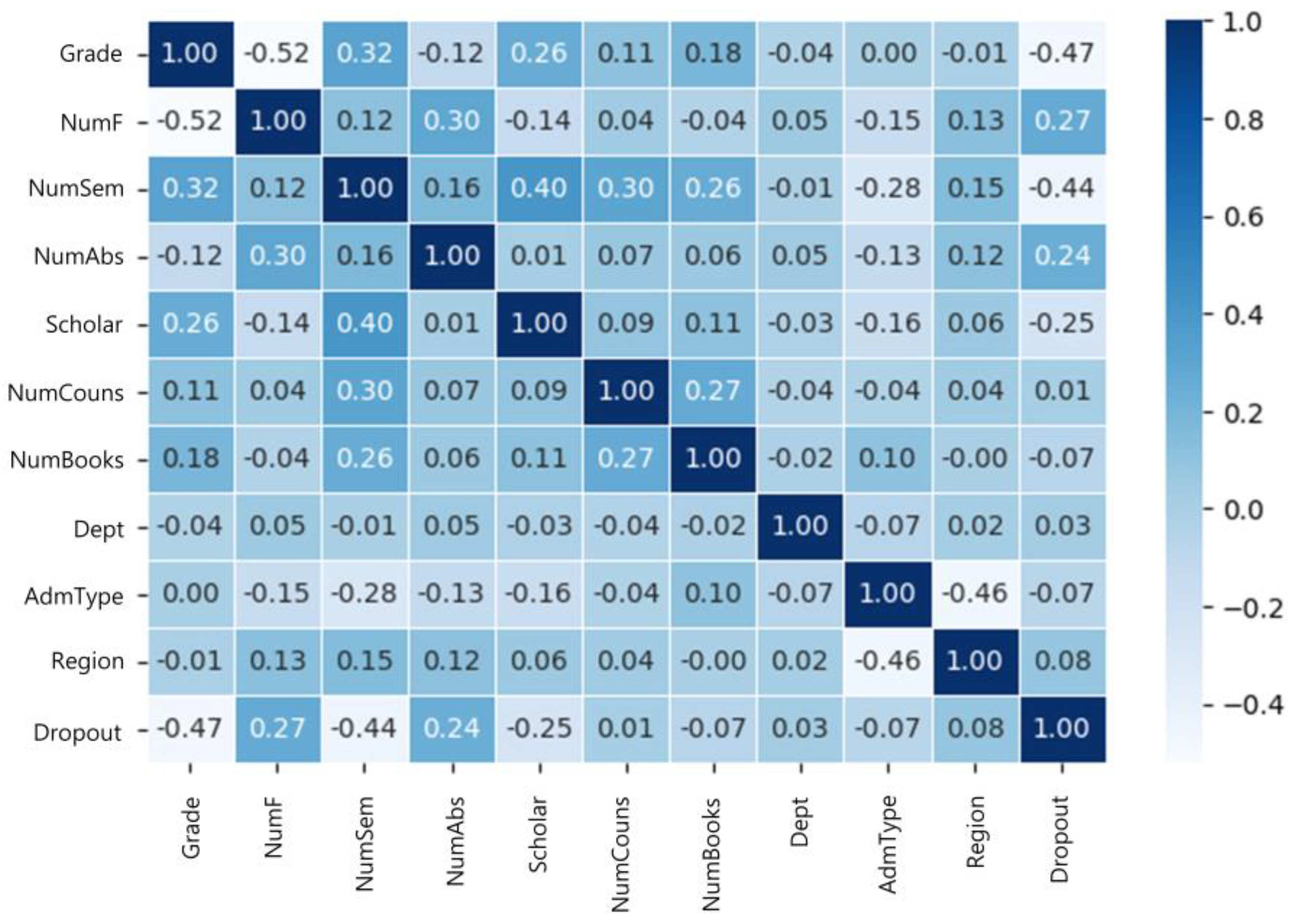
Regarding ②, the summary table can arithmetically contain up to 150 attributes. In order to achieve high classification accuracy, only attributes that have a high correlation with the Dropout attribute need to be added to the table; the more attributes that are highly correlated with student dropout are included and learned, the higher prediction accuracy can be obtained. As a criterion for the selection, the correlation coefficient with the Dropout attribute was examined for each candidate. In the proposed method, attributes whose coefficient value was greater than or equal to 0.01 were chosen.
Figure 1 shows the attributes chosen for the summary table. The attribute with the highest correlation with Dropout was Grade, followed by NumSem, NumF, Scholar, and NumAbs. NumSem was highly correlated with Grade and Scholar, while Grade was highly correlated with NumF. To obtain the correlation coefficients between the attributes, the corr() function of the data frame in Python was used. For visualization, the heatmap() function in the Seaborn package [35] was used.
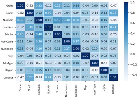
Figure 1.
Selected attributes for the summary table whose correlation coefficient with the Dropout attribute is greater than or equal to 0.01.
Table 6 shows an example of the summary table constructed from the records shown in Table 3 and Table 4. The summary table consists of 11 attributes shown in Figure 1 in addition to SID as a primary key, and it has 20,050 records, which is equal to the number of students registered in the academic information system of Sahmyook University.

Table 6.
Example records of the summary table with key attributes extracted from the source tables shown in Table 2.
3.3. Model Implementation
As an algorithm to build a model for the dropout prediction, various machine learning algorithms were used and compared, including Logistic Regression (LR), Decision Tree (DT), Random Forest (RF), Support Vector Machine (SVM), Deep Neural Network (DNN), and Light Gradient Boosting Machine (LightGBM). For the LR, DT, RF, SVM, and LightGBM models, Scikit-learn [36] was used, which is a machine learning library in Python. For the DNN models, Keras [37] was used, which is an open source software library for artificial neural networks provided by Google.
The summary table shown in Table 6 is used as input data for training the model. The table is input in the form of a CSV file and converted to a data frame in Python. From the data frame, the X and T lists are extracted as follows, which denote the list of input records and the list of values indicating whether each input record results in dropout or not, respectively. Since there is a derivation between the values of X, its values are normalized to values between 0 and 1 using Scikit-learn’s StandardScaler. Then, X and T are split into the training and test data sets using the train_test_split() function. In the code below, X_train and T_train denote the training data sets, while X_test and T_test denote the test data sets.
| X = df[[“AdmType”,”NumSem”,”Grade”, … ]].values T = df[“Dropout”].values X_scaled = StandardScaler().fit_transform(X) X_train, X_test, T_train, T_test = train_test_split(X_scaled, T, test_size = 0.2) |
Table 7 shows the hyperparameters and their settings for each machine learning algorithm used to implement the model. First, the LR model was implemented using the LogisticRegression class, which is included in the linear_model package of Scikit-learn. The value of C, the regularization parameter used to control overfitting, was set to 100.
| from sklearn.linear_model import LogisticRegression model = LogisticRegression(C = 100) model.fit(X_train, T_train) |

Table 7.
Hyperparameter settings of machine learning algorithms used to implement the dropout prediction model in the proposed method.
The DT model was implemented using the DecisionTreeClassifier class included in the tree package of Scikit-learn. The parameter max_depth was set to 10, which denotes the depth of a Decision Tree to control overfitting. The parameter random_state was set to 0 to get the same Decision Tree when conducting experiments.
| from sklearn.tree import DecisionTreeClassifier model = DecisionTreeClassifier(max_depth = 10, random_state = 0) model.fit(X_train, T_train) |
The RF model was implemented using the RandomForestClassifier class included in the ensemble package of Scikit-learn. The parameter n_estimators was set to 100, which represents the number of trees that make up a forest, and the parameter random_state was set to 0 to get the same forest when conducting experiments.
| from sklearn.ensemble import RandomForestClassifier model = RandomForestClassifier(n_estimators = 100, random_state = 0) model.fit(X_train, T_train) |
The SVM model was implemented using the SVC class included in the svm package of Scikit-learn. The parameter C was set to 100, the same as for the LR model.
| from sklearn.svm import SVC model = SVC(C = 100) model.fit(X_train, T_train) |
The DNN model was implemented using Keras 2.0 and consisted of three Dense layers. The Dense layer has two parameters to specify the number of hidden nodes and the activation function. For the first two layers, relu was used as an activation function to calculate the output value from each node while avoiding the vanishing gradient problem [38]. For the last layer, sigmoid was used as an activation function to calculate the probability of student dropout. The parameter input_shape in the first layer was used to specify the size of input data. As an optimizer for the DNN model, adam was used, and binary-crossentropy was adopted as a loss function to correct the weights and biases based on the T values. The training was set to be performed up to 50 times.
| model = keras.Sequential([ keras.layers.Dense(128, activation = “relu”, input_shape = (7, )), keras.layers.Dense(32, activation = “relu”), keras.layers.Dense(1, activation = ‘sigmoid’) ]) model.compile(optimizer = “adam”, loss = ‘binary_crossentropy’) model.fit(X_train, T_train, epochs = 30) |
The LightGBM model was implemented using the LGBMClassifier class included in the lightgbm package. The parameter n_estimators was set to 100, which represents the number of boosted trees, and the parameter random_state was set to 0 to get the same data when conducting experiments.
| from lightgbm import LGBMClassifier model = LGBMClassifier(n_estimators = 100, random_state = 0) model.fit(X_train, T_train) |
4. Experimental Results
4.1. Performance Measure
Dropout prediction is a two-class classification problem, where dropout records are classified into the P (Positive) class, while non-dropout records are classified into the N (Negative) class. When evaluating the prediction result, T (True) means that the prediction is correct, and F (False) means that it is not. From this, there are four cases for determining the prediction performance in the two-class classification problem, including TP (True Positive), FP (False Positive), FN (False Negative), and TN (True Negative). In the prediction of student dropout, TP refers to a case where the model correctly predicts the P class, i.e., student dropout, while FP refers to a case where the model incorrectly predicts the dropout. TN and FN can be interpreted in the same way.
The most common measure to evaluate the prediction performance is accuracy, which is defined as follows.
Note that when the data are skewed toward one class, accuracy cannot be used properly. For example, the dropout rate of four-year universities in South Korea is about 5% [6,7], where the data are highly skewed to the N class. In this case, simply predicting that no one will drop out would yield 95% accuracy. However, if the opposite prediction is made, the accuracy is significantly lowered to 5%.
The above problem indicates that FP and FN should be used together when measuring the prediction performance. Precision can be used to measure the performance from the perspective of FP and is defined as
Similarly, recall can be used to measure the performance from the perspective of FN, which is defined as
A simple way to measure the performance considering both FP and FN is to use the average of precision and recall. The F1-score is defined as the harmonic mean of precision and recall as follows.
In this paper, the F1-score was used for evaluating the performance of prediction models since it can properly reflect the data imbalance in the performance evaluation.
4.2. Model Performance
To check the performance of prediction models implemented with LR, DT, RF, SVM, DNN, and LightGBM, which were discussed in Section 3.3, experiments were conducted on the summary table with the 20,050 student records shown in Table 6. The experiments were performed on an HP server equipped with an Intel Xeon E5-2609 1.70 GHz CPU, MSI GeForce RTX-4090 GPU, and 32 GB of memory. TensorFlow 2.10.1 was used for DNN, and CUDA 11.8 was used for GPU acceleration.
Table 8 shows the prediction performance of the six models, where each value in the table represents the average value of 5 runs obtained through the experiments. The average accuracy of the six models was high at 0.945, while their average F1-score was relatively low at 0.796. Among the models, the LightGBM model showed the highest prediction performance with an F1-score of 0.840.

Table 8.
Prediction performance of the LR, DT, RF, SVM, and DNN models discussed in Section 3.3.
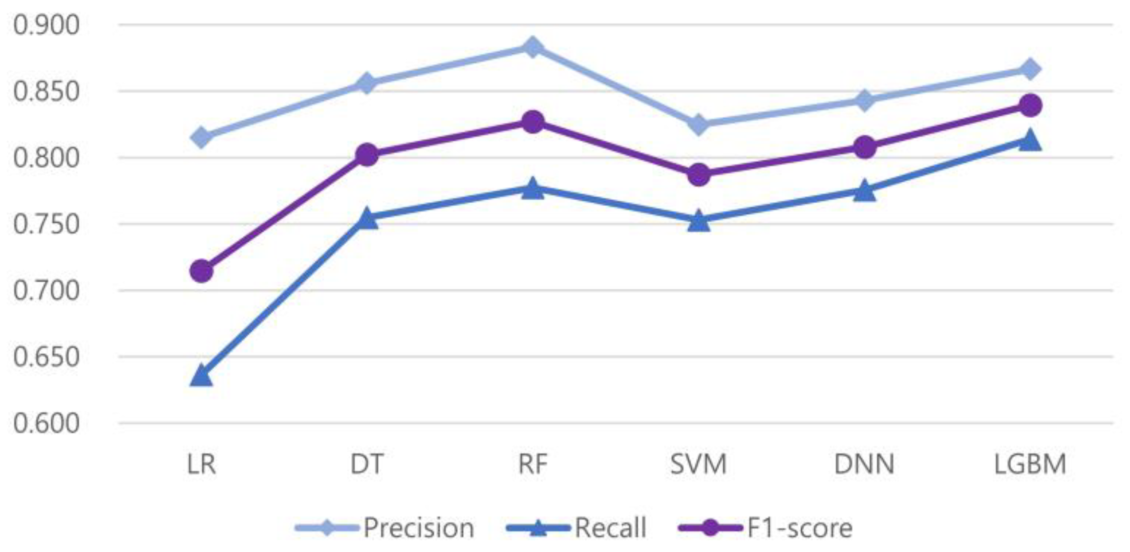
Figure 2 depicts the differences between the precision, recall, and F1-scores of the six models. We can see that the graph of the F1-score is more affected by recall than precision; the difference between the F1-score and recall values is smaller than the difference between the F1-score and precision values. The standard deviation of recalls is also larger than that of precisions, which is shown in Table 8.
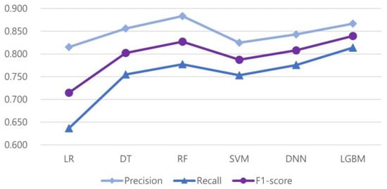
Figure 2.
Precision, recall, and F1-scores of the proposed prediction models.
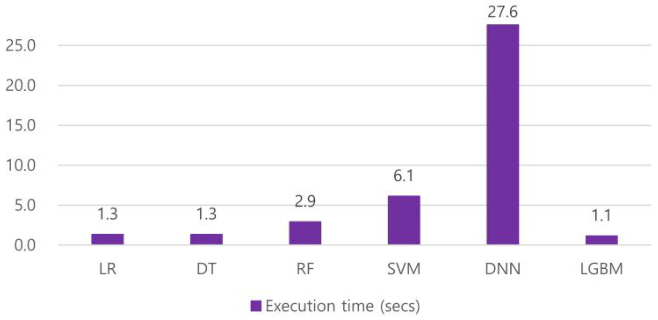
Figure 3 compares the average execution time of the six models. The LR, DT, RF, and LightGBM models showed relatively good performance within 3 s, while the SVM and DNN models have longer execution times. Especially in the case of the DNN model, it took over 27 s to run 30 epochs.

Figure 3.
Average execution time of the LR, DT, RF, SVM, DNN, and LightGBM models.
Considering the prediction accuracy and execution time of the six models obtained through the experiments, the LightGBM model showed the best performance and is expected to be most suitable for the dropout prediction. Table 9 compares the performance of the proposed LightGBM model with the models presented in previous studies. As discussed in Section 2, the models of [8,9,29,30,32] were compared. In [8], an F1-score of 0.808 was obtained using an ensemble model of CatBoost and XGBoost. In [9], the performance of the ridge regression model was the best, providing a precision of 0.739. In [29], the RF model provided the best performance with an F1-score of 0.810. In [30], the SVM model was the best, providing an F1-score of 0.804. In [32], the DNN model achieved an accuracy of 0.768. Compared to the five existing models, the proposed LightGBM model showed improved performance in all aspects with accuracy, precision, and F1-score of 0.955, 0.867, and 0.840, respectively.

Table 9.
Performance comparison of the proposed LightGBM model and the existing models discussed in [8,9,29,30,32].
4.3. Influence of Oversampling
As mentioned earlier, the source data used for dropout prediction are highly skewed, where the dropout records account for only 5% of the total data. Such data imbalance can have a significant impact on the prediction performance because it can lead to an overfitting problem where the training can be biased toward a class with a higher distribution. For example, the ratio of P and N classes in our source data is 5:95. In this case, the training can be biased toward the N class, which leads to the result that the prediction performance for the N class increases while the performance for the P class may significantly decrease.
One of the popular methods to resolve the overfitting problem is oversampling. In this technique, artificial records are generated and added to the minor class, e.g., the P class, until the ratio between the classes becomes even. Among the various oversampling techniques, SMOTE (Synthetic Minority Oversampling Technique) [20] is the most commonly used.
Data augmentation in SMOTE is performed based on K-NN. Figure 4 illustrates how artificial records are generated in SMOTE. It considers only the records in the P class when generating new records. From the P class data, a reference vector is first selected. Then, K neighboring vectors close to the reference vector are chosen using K-NN. These vectors are connected to the reference vector with lines, as shown in Figure 4. Finally, new vectors are randomly extracted from the connection lines and added to the minor class until the ratio between the classes becomes even.
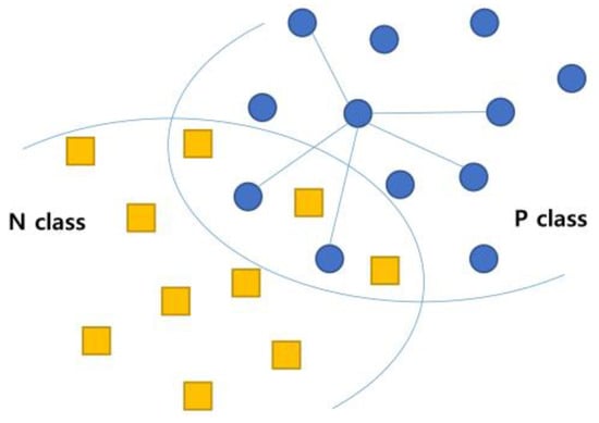
Figure 4.
Data augmentation in SMOTE.
Table 10 shows the prediction performance when SMOTE is applied to the proposed prediction models. SMOTE was applied only to the training data, not to the test data. From the results shown in Table 10, we can see that the F1-scores of all models except the RF model decreased after applying SMOTE. Compared with the results in Table 8, the average F1-score of the models dropped from 0.796 to 0.762. This is due to the fact that the average value of precision has dropped significantly from 0.848 to 0.677. On the other hand, the average value of recall improved from 0.752 to 0.882. As an exceptional case, the F1-score of the RF model slightly increased from 0.827 to 0.830. It was not possible to measure the performance of the LightGBM model since an error occurred due to a conflict between the LightGBM and SMOTE packages.

Table 10.
Performance of the proposed prediction models after applying SMOTE.
We also checked the influence of ADASYN and Borderline-SMOTE on the performance of the proposed prediction models. Table 11 and Table 12 show the performance after ADASYN and Borderline-SMOTE were applied, respectively. ADASYN showed the lowest performance, with an average F1-score of 0.735, among the three oversampling techniques discussed in this paper. The performance of Borderline-SMOTE was also worse than that of SMOTE, with an average F1-score of 0.742.

Table 11.
Performance of the proposed prediction models after applying ADASYN.

Table 12.
Performance of the proposed prediction models after applying Borderline-SMOTE.
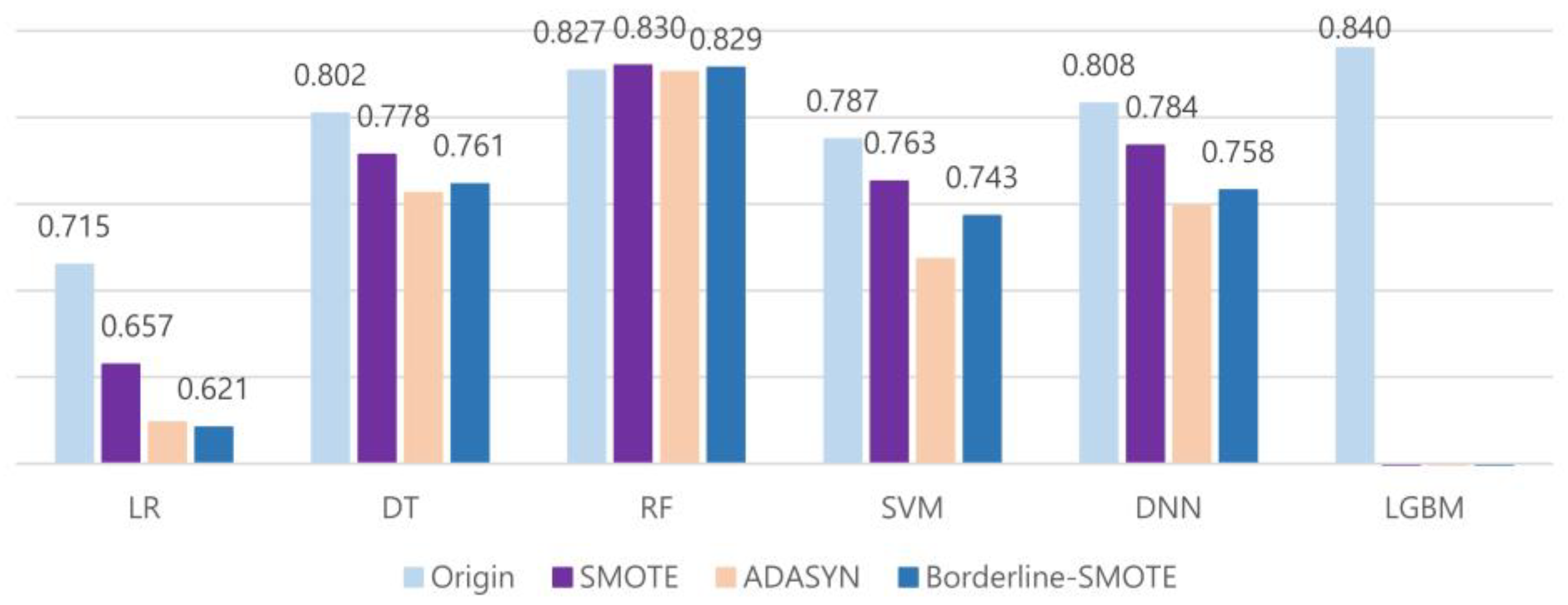
Figure 5 visualizes the change in F1-scores of the proposed prediction models before and after applying SMOTE, ADASYN, and Borderline-SMOTE. The average F1-scores of all models decreased after applying the oversampling techniques, except the RF model; the performance improvement of the RF model was also not so significant. Among the oversampling techniques, SMOTE showed the best performance, whereas ADASYN performed the worst.
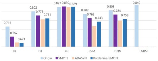
Figure 5.
Change in F1-scores of the proposed prediction models before and after applying SMOTE, ADASYN, and Borderline-SMOTE.
The performance degradation after applying oversampling was also discussed in the previous studies of [39,40]. The reason can be explained by the fact that the new dropout records of the P class augmented by SMOTE or other techniques acted as noise when the classification process was performed. As shown in Figure 4, as the overlapping region between the P and N classes increases, classification becomes more difficult.
To see how much portion of our source data overlaps, we compared the data distribution of dropout and non-dropout students. Among the 10 attributes used for training, we examined the distribution of grades and the number of leaves of absence, which had a high correlation with student dropout. Figure 6 shows the distribution of the two attribute values for students in the Computer Science department of Sahmyook University, where purple circles denote the values of dropout students while yellow circles denote the values of non-dropout students. As shown in the figure, the data of the two groups significantly overlapped in the areas where the grade ranges from 1.0 to 4.0, and the number of absences ranges from 1 to 4 semesters. In this case, if dropout records are oversampled and added to the P class, the number of FP errors might increase significantly, which can subsequently decrease the precision of the prediction models.
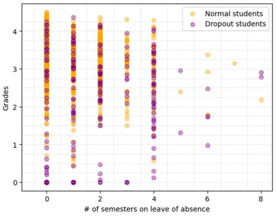
Figure 6.
Distribution of grades and number of semesters on leave of absence for dropout and non-dropout students in the Department of Computer Engineering of Sahmyook University.
5. Conclusions and Future Work
In this study, we implemented machine learning models to predict the dropout of university students and compared the performance of the models using academic records collected from 20,050 students at Sahmyook University located in Seoul, Republic of Korea. Since the source records were stored in multiple tables separately to avoid redundancy, the records from the tables were merged into a single table with 150 attributes to perform learning. Among them, 10 attributes having a high correlation with student dropout were extracted and used for learning. To implement a prediction model, various machine learning algorithms, including Linear Regression, Decision Tree, Random Forest, Support Vector Machine, Deep Neural Network, and Light Gradient Boosting Machine (LightGBM), were used. The performance of the models was compared through experiments, and the LightGBM model provided the best performance with an F1-score of 0.840.
We also examined the influence of the data imbalance on the prediction performance. For this purpose, we compared the performance of the proposed prediction models before and after applying oversampling techniques such as SMOTE, ADASYN, and Borderline-SMOTE. Interestingly, the performance of all models decreased after applying the oversampling techniques, except the RF model, and the performance improvement of the RF model was also not so significant. Among the oversampling techniques, SMOTE showed the best performance, whereas ADASYN performed the worst.
Such performance degradation means that there was a lot of overlap in the data between the dropout and non-dropout classes. From this, new records augmented by the oversampling techniques acted as noise when the classification process was performed. Regarding this, we plan to study oversampling techniques that can reduce noise by detecting the class boundary or outliers more clearly. We will also continue research to develop a new model that can predict student dropout by semester.
Author Contributions
Methodology, C.H.C. and Y.W.Y.; Writing—original draft, H.G.K. All authors have read and agreed to the published version of the manuscript.
Funding
This research was supported by the Sahmyook University Research Fund in 2023.
Institutional Review Board Statement
Not applicable.
Informed Consent Statement
Not applicable.
Conflicts of Interest
The authors declare no conflict of interest. The funders had no role in the design of the study; in the collection, analyses, or interpretation of data; in the writing of the manuscript; or in the decision to publish the results.
References
- Kim, D.; Kim, S. Sustainable education: Analyzing the determinants of university student dropout by nonlinear panel data models. Sustainability 2018, 10, 954. [Google Scholar] [CrossRef]
- Martinho, V.R.D.C.; Nunes, C.; Minussi, C.R. An intelligent system for prediction of school dropout risk group in higher education classroom based on artificial neural networks. In Proceedings of the 2013 IEEE 25th International Conference on Tools with Artificial Intelligence, Washington, DC, USA, 4–6 November 2013; pp. 159–166. [Google Scholar]
- Jain, P.; Chhabra, H.; Chauhan, U.; Prakash, K.; Gupta, A.; Soliman, M.S.; Islam, M.S.; Islam, M.T. Machine learning assisted hepta band THz metamaterial absorber for biomedical applications. Sci. Rep. 2023, 13, 1792. [Google Scholar] [CrossRef] [PubMed]
- Jain, P.; Chhabra, H.; Chauhan, U.; Singh, D.K.; Anwer, T.M.K.; Ahammad, S.H.; Hossain, M.A.; Rashed, A.N.Z. Multiband Metamaterial absorber with absorption prediction by assisted machine learning. Mater. Chem. Phys. 2023, 307, 128180. [Google Scholar] [CrossRef]
- Prenkaj, B.; Velardi, P.; Stilo, G.; Distante, D.; Faralli, S. A survey of machine learning approaches for student dropout prediction in online courses. ACM Comput. Surv. (CSUR) 2020, 53, 1–34. [Google Scholar] [CrossRef]
- Alyahyan, E.; Düştegör, D. Predicting academic success in higher education: Literature review and best practices. Int. J. Educ. Technol. High. Educ. 2020, 17, 3. [Google Scholar] [CrossRef]
- Mduma, N.; Khamisi, K.; Dina, M. A Survey of Machine Learning Approaches and Techniques for Student Dropout Prediction. Data Sci. J. 2019, 18, 1–10. [Google Scholar] [CrossRef]
- Kim, S.; Choi, E.; Jun, Y.K.; Lee, S. Student Dropout Prediction for University with High Precision and Recall. Appl. Sci. 2023, 13, 6275. [Google Scholar] [CrossRef]
- Jeong, S.H. A study on the development of university students dropout prediction model using classification technique. J. Converg. Cons. 2022, 5, 174–185. [Google Scholar]
- Park, C. Development of prediction model to improve dropout of cyber university. J. Korea Acedemia-Ind. Coop. Soc. 2020, 21, 380–390. [Google Scholar]
- Onah, D.F.; Sinclair, J.; Boyatt, R. Dropout rates of massive open online courses: Behavioral patterns. In Proceedings of the 6th International Conference on Education and New Learning Technologies, Barcelona, Spain, 7–9 July 2014; pp. 5825–5834. [Google Scholar]
- Liyanagunawardena, T.R.; Parslow, P.; Williams, S. Dropout: MOOC participants’perspective. In Proceedings of the EMOOCs 2014, the Second MOOC European Stakeholders Summit, Lausanne, Switzerland, 10–12 February 2014; pp. 95–100. [Google Scholar]
- Xing, W.; Du, D. Dropout prediction in MOOCs: Using deep learning for personalized intervention. J. Educ. Comput. Res. 2019, 57, 547–570. [Google Scholar] [CrossRef]
- McDonald, G.C. Ridge regression. Wiley Interdiscip. Rev. Comput. Stat. 2009, 1, 93–100. [Google Scholar] [CrossRef]
- Quinlan, J.R. Induction of decision trees. Mach. Learn. 1986, 1, 81–106. [Google Scholar] [CrossRef]
- Ho, T.K. Random Decision Forests. In Proceedings of the 3rd International Conference on Document Analysis and Recognition, Montreal, QC, Canada, 14–16 August 1995; pp. 278–282. [Google Scholar]
- Meyer, D.; Wien, F.T. Support vector machines. R News 2001, 1, 23–26. [Google Scholar]
- Schmidhuber, J. Deep learning in neural networks: An overview. Neural Netw. 2015, 61, 85–117. [Google Scholar] [PubMed]
- Ke, G.; Meng, Q.; Finley, T.; Wang, T.; Chen, W.; Ma, W.; Ye, Q.; Liu, T.Y. LightGBM: A highly efficient gradient boosting decision tree. In Proceedings of the 31st Conference on Neural Information Processing Systems (NIPS 2017), Long Beach, CA, USA, 4–9 December 2017; Volume 30. [Google Scholar]
- Chawla, N.V.; Bowyer, K.W.; Hall, L.O.; Kegelmeyer, W.P. SMOTE: Synthetic minority over-sampling technique. Artif. Intell. Res. 2002, 16, 321–357. [Google Scholar] [CrossRef]
- He, H.; Bai, Y.; Garcia, E.A.; Li, S. ADASYN: Adaptive synthetic sampling approach for imbalanced learning. In Proceedings of the 2008 IEEE International Joint Conference on Neural Networks, Hong Kong, China, 1–8 June 2008; pp. 1322–1328. [Google Scholar]
- Han, H.; Wang, W.-Y.; Mao, B.-H. Borderline-SMOTE: A new over-sampling method in imbalanced data sets learning. In Proceedings of the IEEE 2005 International Conference on Advances in Intelligent Computing, Hefei, China, 23–26 August 2005; Volume 16, pp. 878–887. [Google Scholar]
- Barros, T.M.; Souza Neto, P.A.; Silva, I.; Guedes, L.A. Predictive Models for Imbalanced Data: A School Dropout Perspective. Educ. Sci. 2019, 9, 4–275. [Google Scholar] [CrossRef]
- Hido, S.; Kashima, H.; Takahashi, Y. Roughly balanced bagging for imbalanced data. Stat. Anal. Data Min. ASA Data Sci. J. 2009, 2, 412–426. [Google Scholar] [CrossRef]
- Batista, G.E.; Prati, R.C.; Monard, M.C. A study of the behavior of several methods for balancing machine learning training data. ACM SIGKDD Explor. Newsl. 2004, 6, 20–29. [Google Scholar] [CrossRef]
- Chen, T.; Guestrin, C. Xgboost: A scalable tree boosting system. In Proceedings of the 22nd ACM Sigkdd International Conference on Knowledge Discovery and Data Mining, San Francisco, CA, USA, 13 August 2016; pp. 785–794. [Google Scholar]
- Dorogush, A.V.; Ershov, V.; Gulin, A. CatBoost: Gradient boosting with categorical features support. arXiv 2018, arXiv:1810.11363. [Google Scholar]
- Webb, G.I.; Keogh, E.; Miikkulainen, R. Naïve Bayes. Encycl. Mach. Learn. 2010, 15, 713–714. [Google Scholar]
- Da Silva, M.; Diogo, E.; Solteiro, P.; Eduardo, J.; Arsénio, R.; de Moura, O.; Paulo, B.; Barroso, J. Forecasting Students Dropout: A UTAD University Study. Future Internet 2022, 14, 76. [Google Scholar] [CrossRef]
- Fernández-García, A.J.; Preciado, J.C.; Melchor, F.; Rodriguez-Echeverria, R.; Conejero, J.M.; Sánchez-Figueroa, F. A real-life machine learning experience for predicting university dropout at different stages using academic data. IEEE Access 2021, 9, 133076–133090. [Google Scholar] [CrossRef]
- Friedman, J.H. Greedy function approximation: A gradient boosting machine. Ann. Stat. 2001, 29, 1189–1232. [Google Scholar] [CrossRef]
- Sandoval-Palis, I.; Naranjo, D.; Vidal, J.; Gilar-Corbi, R. Early Dropout Prediction Model: A Case Study of University Leveling Course Students. Sustainability 2020, 12, 9314. [Google Scholar] [CrossRef]
- Shynarbek, N.; Orynbassar, A.; Sapazhanov, Y.; Kadyrov, S. Prediction of Student’s Dropout from a University Program. In Proceedings of the 16th International Conference on Electronics Computer and Computation (ICECCO), Kaskelen, Kazakhstan, 25–26 November 2021; pp. 1–4. [Google Scholar]
- Exponential Smoothing. Available online: https://en.wikipedia.org/wiki/Exponential_smoothing (accessed on 28 August 2023).
- Seaborn, Statistical Data Visualization. Available online: https://seaborn.pydata.org (accessed on 28 August 2023).
- Scikit-Learn. Available online: https://en.wikipedia.org/wiki/Scikit-learn (accessed on 28 August 2023).
- Keras. Available online: https://www.tensorflow.org/guide/keras (accessed on 28 August 2023).
- Hu, Z.; Zhang, J.; Ge, Y. Handling vanishing gradient problem using artificial derivative. IEEE Access 2021, 9, 22371–22377. [Google Scholar] [CrossRef]
- Lee, S.; Chung, J.Y. The machine learning-based dropout early warning system for improving the performance of dropout prediction. Appl. Sci. 2019, 9, 3093. [Google Scholar] [CrossRef]
- Moon, G.B.; Kim, J.W.; Lee, J.S. Early prediction model of student performance based on deep neural network using massive LMS log data. J. Korea Contents Assoc. 2021, 21, 10. [Google Scholar]
Disclaimer/Publisher’s Note: The statements, opinions and data contained in all publications are solely those of the individual author(s) and contributor(s) and not of MDPI and/or the editor(s). MDPI and/or the editor(s) disclaim responsibility for any injury to people or property resulting from any ideas, methods, instructions or products referred to in the content. |
© 2023 by the authors. Licensee MDPI, Basel, Switzerland. This article is an open access article distributed under the terms and conditions of the Creative Commons Attribution (CC BY) license (https://creativecommons.org/licenses/by/4.0/).

