Article

Mechanical Performance Prediction Model of Steel Bridge Deck Pavement System Based on XGBoost

1
Henan Puwei Expressway Company Limited, Puyang 457000, China
2
School of Water Conservancy and Transportation, Zhengzhou University, Zhengzhou 450001, China
3
School of Civil Engineering, Wuhan University, Wuhan 430072, China
*
Author to whom correspondence should be addressed.
Appl. Sci. 2023, 13(21), 12048; https://doi.org/10.3390/app132112048
Submission received: 13 September 2023 / Revised: 23 October 2023 / Accepted: 30 October 2023 / Published: 5 November 2023
(This article belongs to the Section Civil Engineering)

Abstract

:
Steel bridges are widely used in bridge engineering. In the structural design of steel bridge deck pavement systems, engineers focus on obtaining mechanical properties by calculating design parameters and are keen to establish a quick and accurate solution method. Because of the complex knowledge system involved in the numerical calculation method, it is difficult for the general engineering designer to master it. Researchers have started using artificial intelligence algorithms to solve problems in civil engineering. This study developed an XGBoost-based mechanical performance prediction model for steel bridge deck pavement systems. First, numerical simulation tests are conducted at unfavorable load locations using a finite element model to establish a dataset. Then, an XGBoost model is built using this dataset, and its parameters are optimized and compared with traditional machine learning models. Finally, an explanatory analysis of the model is performed using SHAP, an interpretable machine learning framework. The results indicate that the developed XGBoost model accurately predicts the mechanical properties of steel bridge deck pavement systems.

1. Introduction

Steel box girder bridges are widely used in bridge engineering due to their large spans, short construction periods, and ease of transportation. The steel deck pavement system comprises orthotropic anisotropic steel bridge panels and asphalt concrete pavement layers that differ in characteristics from ordinary highway asphalt concrete pavements [1,2]. The asphalt concrete pavement layer is laid directly on the steel bridge deck. Due to the flexibility of the steel deck, the force and deformation of the pavement layer become more complex under various factors such as vehicle load and the climatic environment [3,4,5]. In recent years, China’s traffic volume has continued to grow along with an increase in heavy traffic. As a result, some steel bridge deck pavements have begun to exhibit transverse and longitudinal cracking, rutting, pushing, congestion, and other issues. Traffic management departments have had to invest significant time and manpower into maintaining these pavements. Delayed maintenance can lead to greater safety hazards and economic losses [6,7].
In the structural design of steel bridge deck pavement systems, engineers focus on obtaining mechanical properties by calculating design parameters and are keen to establish a quick and accurate solution method. Battista et al. studied the fatigue cracking of steel deck pavement systems under vehicle loading using finite element software and experiments under static and dynamic effects [8]. Seim et al. conducted numerical simulation tests using the finite element model of a steel deck pavement system to obtain the fatigue cracking of the steel deck pavement system by varying the thickness of the pavement layer. They also obtained variations in the mechanical properties of the steel deck pavement system under vehicle loading by a varying thickness and elastic modulus of the pavement layer [9]. Kim et al. adjusted structural design parameters using a finite element model of the steel deck pavement system to obtain variations in the mechanical properties of the steel deck pavement system under vehicle loading [10].
Due to the complex knowledge system involved in numerical calculation methods and their long learning period, it is difficult for general engineering designers to master them proficiently. The accuracy of numerical calculation results is highly dependent on operator experience. Additionally, numerical calculation methods depend on intrinsic model accuracy and numerical calculation algorithm efficiency. When calculating refined models, classical method modeling and solving will take a longer time. Therefore, classical numerical computational analysis methods have significant room for improvement in terms of parameterization and computational efficiency [11]. Artificial intelligence techniques such as machine learning algorithms are gradually being applied in engineering. Data-driven artificial intelligence techniques can break through artificial empirical perception and eliminate dependence on humans [12,13]. Integrated learning methods represented by XGBoost models have become increasingly popular among researchers in engineering prediction problems in recent years [14,15]. Lyngdoh et al. used several popular machine learning models for concrete strength prediction. Their study showed that the XGBoost model has a superior performance [16]. Nguyen-Sy et al. established a model based on the XGBoost model for predicting the compressive strength of concrete. Their study showed that the XGBoost model has a higher accuracy compared to other existing machine learning models [17]. Liang et al. used GBDT, XGBoost, and LightGBM models to predict the stability of hard rock pillars. The results showed that all three algorithms have a better performance [18]. Feng et al. used four integrated learning models to predict the shear strength of reinforced concrete beams with and without web reinforcement. The developed models all show a better performance in predicting shear strength and outperform traditional machine learning methods [19]. Bakouregui et al. used the XGBoost model to predict the load-carrying capacity of FRP-reinforced concrete columns. They also analyzed the model for interpretability using SHAP architecture. The results of the study showed that the proposed prediction model has a better performance [20]. Chen et al. assessed the seismic vulnerability of buildings in Kavrepalanchok, Nepal, using the XGBoost model. The developed model has a high accuracy [21].
No research has been conducted to establish a prediction model between the mechanical performance index of pavement systems and the structural design parameters using machine learning algorithms. This study aims to fill this gap by developing an XGBoost-based mechanical performance prediction model for steel bridge deck pavement systems. This study focuses on the following aspects: (1) establishing the dataset by conducting numerical simulation tests at the most unfavorable load locations using a finite element model; (2) establishing the XGBoost model and optimizing its parameters; (3) comparing the XGBoost model with traditional machine learning models to evaluate its accuracy; and (4) using the SHAP framework to perform explanatory analysis. The technical route is shown in Figure 1.

2. Method

2.1. XGBoost (Extreme Gradient Boosting)

Integrated learning methods are used to obtain better predictions by fusing multiple base learners and combining them [22]. Boosting is the most dominant class of integrated learning methods. Boosting first uses the dataset for training to obtain a base learner. It then observes the results of this base learner training and assigns more attention to the training samples that do wrong in it. This adjusted training set is then used to train the next base learner, and so on until the set number of base learners is reached. Finally, these base learners are weighted together [23]. The XGBoost algorithm is one of the best-performing algorithms in the Boosting family. The loss function of the XGBoost algorithm uses a second-order Taylor expansion to improve the accuracy [24]. For each parameter (learning_rate), its value range is generally from 0 to 1. For parameter (n_estimators), its value range needs to be set appropriately based on sample size and feature count. For parameter (max_depth), it can be unrestricted when the sample size and feature count are small, but should be set within reasonable bounds when they are large. For parameter (min_child_weight), its value cannot be too large or too small; too small will result in overfitting, while too large will result in underfitting.

2.2. SHAP (Shapley Additive Explanations)

Most current machine learning models are black-box models, which can only provide prediction results without interpretable analyses of the models. To address this issue, methods are needed to analyze the interpretability of machine learning models. SHAP is an interpretability analysis method based on the Shapley value in game theory, which aims to explain machine learning models [25,26]. The SHAP architecture can be used to determine the degree of influence of each feature variable on the prediction results of the model [27].

3. Dataset Creation

To establish a prediction model of the mechanical performance index of the steel bridge deck pavement system using machine learning algorithms, datasets are required to provide data support. Numerical simulation tests are conducted at the most unfavorable load location using a finite element model to obtain these datasets. Different combinations of design parameters were then considered under the most unfavorable load position, and the orthogonal design method was used to numerically simulate the deck system. Finally, numerical simulation results were used to establish a mechanical performance index dataset for steel deck pavement systems.

3.1. Finite Element Modeling

When analyzing the mechanical properties of the steel deck pavement system using the finite element method, a local model is typically used as the computational model. Therefore, this study uses a local model of the steel deck pavement system for calculation and analysis. The bridge under consideration is Highway Mainline Bridge No. 1, which is 2.8 m high and 16.31 m wide. The standard cross-section of a steel box girder is shown in Figure 2. The standard thickness of the steel box girder top plate is 16 mm, while that of the bottom plate is 14 mm. The top plate stiffening ribs are U-shaped stiffening ribs. The whole bridge model is simplified to obtain the local finite element model, which has a size of 4200 mm × 9000 mm and includes seven U-shaped stiffening ribs and four cross-sectional plates. The steel structure, such as the steel bridge deck, U-shaped stiffening ribs, and cross-partitions, are in shell units, while the pavement layer is in solid units. Table 1 shows the parameters of the local finite element model of the steel deck pavement system.
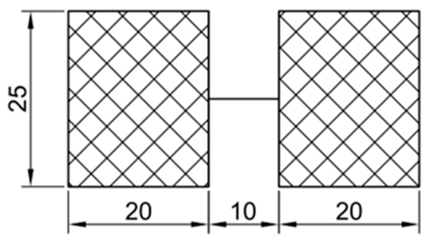
According to the Specification for the Design of Highway Steel Bridges (JTGD64-2015), the load type for a single-axle two-wheel set is selected as 140 KN, and the two-wheel tire load weighs 70 KN [28]. Assuming that the vehicle load is uniformly distributed on the contact surface between the tires and the pavement, the contact pressure is related to the contact area. The contact surface is simplified to a rectangle, and the load equivalent action form is shown in Figure 3. The boundary conditions of the finite element model are as follows: the horizontal displacement of the steel bridge panel and pavement is restricted, while the vertical displacement is not restricted. The bottom of the cross-partition is solidified. The number of elements is 20,624. The number of elements nodes is 30,142. The finite element model is shown in Figure 4.

3.2. The Most Unfavorable Load Position

To investigate the changes in the force of the pavement system when the load acts on the bridge deck at different positions in the transverse and longitudinal directions, a simulation test was conducted by controlling the relative positions of the load concerning the U-shaped ribs and the transverse spacer. Three cases of transverse load position were set based on the relative position of the load position and the U-shaped stiffening ribs, as shown in Figure 5: (1) the centerline of the load acts directly above the center of the U-shaped stiffening rib; (2) the centerline of the load acts directly above the connection between the U-shaped stiffening ribs and the steel bridge panel; and (3) the centerline of the load acts directly above the centerline of two adjacent U-shaped stiffening ribs. Six cases of longitudinal load position were set based on the relative position of the load position and cross-sectional plate, as shown in Figure 6. The centerline of the load position is 0 mm, 300 mm, 600 mm, 900 mm, 1200 mm, and 1500 mm, respectively, from directly above the cross-partition.
In this study, the maximum transverse tensile stress A1(MPa) on the surface of the pavement, the maximum longitudinal tensile stress A2(MPa) on the surface of the pavement, the maximum transverse shear stress B1(MPa) between the pavement and the steel bridge deck, the maximum longitudinal shear stress B2(MPa) between the pavement and the steel bridge deck, and the maximum vertical displacement C(mm) of the pavement were used as the control indexes of the mechanical properties of the steel bridge deck pavement. The results of the calculation of the mechanical properties of the steel deck pavement system are shown in Table 2.
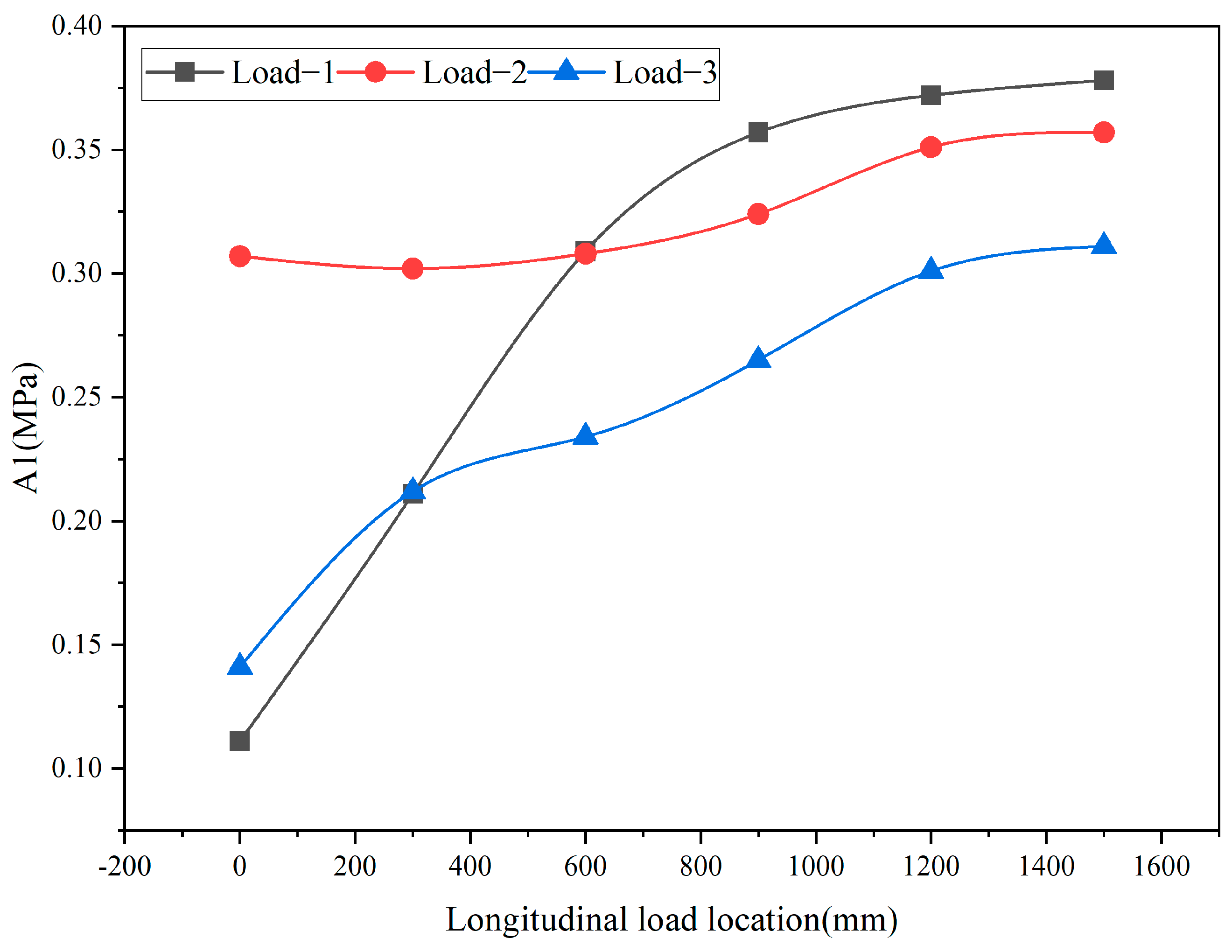
The relationship between the maximum transverse tensile stress on the surface of the paving layer and the longitudinal load position under different transverse load positions is plotted, as shown in Figure 7. From the figure, it can be seen that the most unfavorable load position of the maximum transverse tensile stress on the surface of the paving layer is at transverse load position one (longitudinal 1500 mm). From the transverse partition to the span, the maximum transverse tensile stress on the surface of the paving layer shows a gradually increasing trend. In the distance from 0 mm to 600 mm in the longitudinal direction, transverse load level two is much larger than transverse load level one and load level three. The difference between the maximum transverse tensile stress on the pavement surface at transverse load level two (longitudinal 1500 mm) and transverse load level one (longitudinal 1500 mm) is 5%.
The relationship between the maximum longitudinal tensile stress on the surface of the paving layer and the longitudinal load position under different transverse load positions was plotted as shown in Figure 8. From the figure, it can be seen that the most unfavorable load position of the maximum longitudinal tensile stress on the surface of the paving layer is at transverse load position two (300 mm longitudinal). From the transverse partition to the middle of the span, the maximum longitudinal tensile stress on the surface of the paving layer tends to increase first and then decrease.
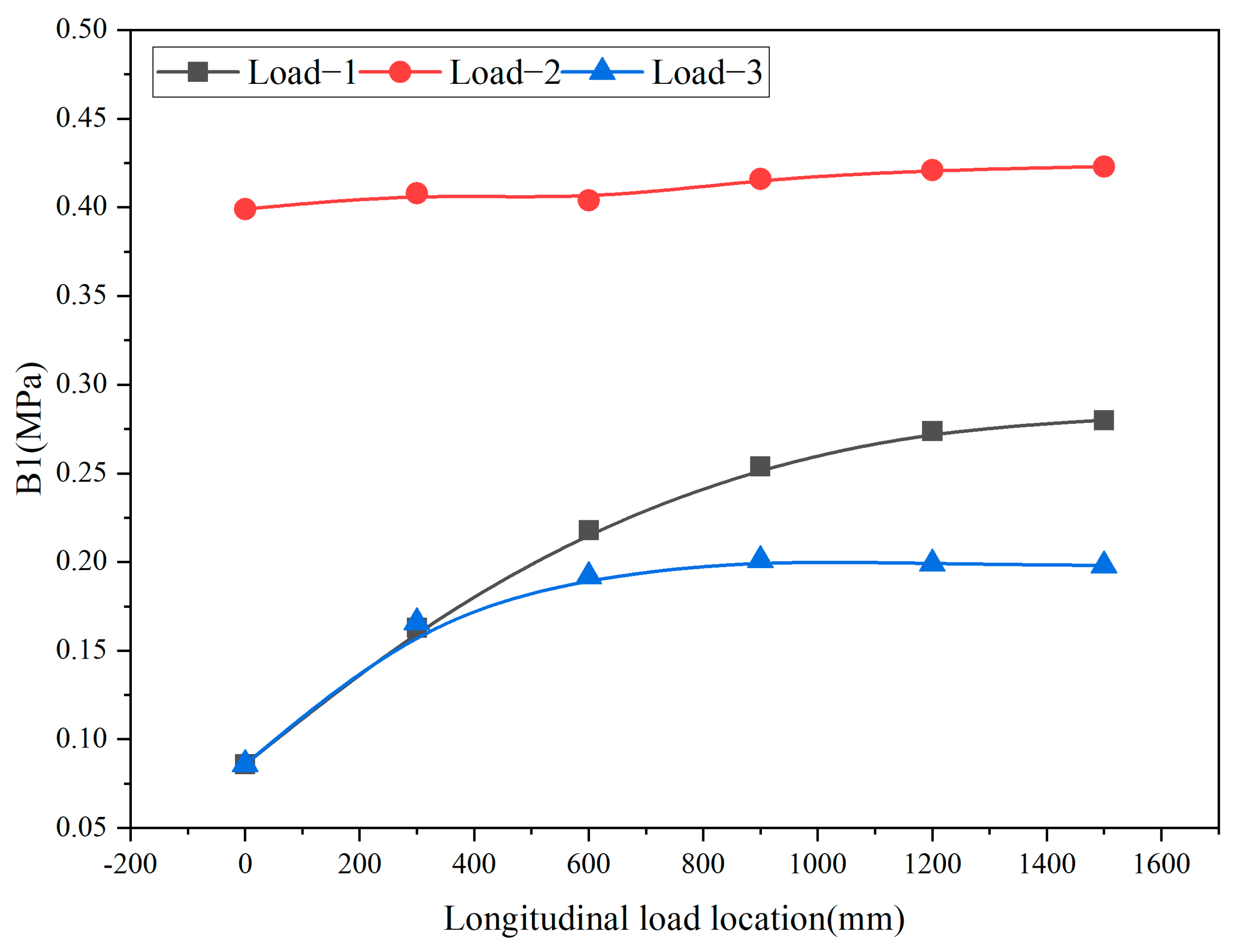
The maximum transverse shear stress between the paving layer and the steel bridge panel under different transverse load positions was plotted against the longitudinal load position, as shown in Figure 9. From the figure, it can be seen that the most unfavorable load position of the maximum transverse shear stress between the pavement and steel bridge panel is at transverse load position two (longitudinal 1500 mm). The maximum transverse shear stress between the paving layer and the steel bridge panel tends to increase gradually from the transverse partition to the middle of the span. The maximum transverse shear stress between the pavement and the steel bridge deck at transverse load position two is much higher than the other transverse load positions.
The relationship between the maximum longitudinal shear stress and longitudinal load position between the paving layer and the steel bridge panel under different transverse load positions is plotted, as shown in Figure 10. From the figure, it can be seen that the most unfavorable load position of the maximum longitudinal shear stress between the pavement and the steel bridge panel is at transverse load position two (longitudinal 1500 mm). The maximum longitudinal shear stress between the paving layer and the steel bridge panel tends to increase gradually from the transverse partition to the middle of the span. The maximum longitudinal shear stress between the pavement and the steel bridge deck at transverse load position two is much higher than the other transverse load positions.
The maximum vertical displacement of the paving layer under different transverse load positions is plotted against the longitudinal load position, as shown in Figure 11. From the figure, it can be seen that the most unfavorable load position of the maximum vertical displacement of the paving layer is at transverse load position one (longitudinal 1500 mm). From the transverse partition to the middle of the span, the maximum vertical displacement of the pavement layer shows a gradually increasing trend. The difference between the maximum vertical displacement of the pavement at transverse load position two (longitudinal 1500 mm) and transverse load position one (longitudinal 1500 mm) is 1%.
It seems that the maximum shear stress between the pavement and steel bridge panel at transverse load position two (longitudinal 1500 mm) is more different than other load positions, and the difference between other mechanical property indexes and each load position is not very obvious. Therefore, the most unfavorable load position was chosen as transverse load position two (longitudinal 1500 m), and this most unfavorable load position was used uniformly in the subsequent study.

3.3. Orthogonal Test

The orthogonal experimental design method is to select the most representative and comprehensive comparable samples from all the test samples and use these selected samples as the test protocol so that a more comprehensive test result can be achieved with as few trials as possible. The core of the orthogonal test design is the selection of a suitable orthogonal table. The usual notation of the orthogonal table is L n ( a b ) , where L represents the orthogonal table, n represents the number of experiments to be done, a represents the level of test factors, and b represents the maximum number of factors that can be arranged in this orthogonal table. The general steps of orthogonal test design are to first determine the appropriate level size of the test factor variables and factor variables, then select the appropriate orthogonal table and determine the test plan, and finally conduct the test according to the orthogonal table and record the test results.
In this study, the orthogonal test design method is used to determine the numerical simulation test scheme, and the numerical simulation test results are used to establish the dataset of the mechanical performance indexes of the steel bridge deck pavement system. The test factors for the mechanical performance index of the steel deck pavement system were selected as follows: the elastic modulus of the upper layer of pavement E1, the elastic modulus of the lower layer of pavement E2, the thickness of the upper layer of pavement H1, the thickness of the lower layer of pavement H2, the thickness of steel bridge deck T, and the spacing of cross-partition D. The level range of the test factors was determined according to the Technical Specification for the Design and Construction of Highway Steel Bridge Deck Pavement (JTG/T3364-02-2019) and engineering experience [29]. The influencing factors and levels of the test were taken as shown in Table 3. There are six influencing factors of the test, two 9 levels, two 6 levels, one 5 level, and one 3 level. Therefore, the orthogonal table L 81 ( 9 6 ) was selected, and the proposed level method was used for the levels with a high number of factor levels. The experimental protocol was designed according to the orthogonal table, the numerical simulation test was conducted according to the experimental protocol, and 81 sets of data were finally obtained.

4. Predictive Modeling

Based on the XGBoost algorithm, five prediction models were established for maximum transverse tensile stress on the surface of the pavement, maximum longitudinal tensile stress on the surface of the pavement, maximum transverse shear stress between the pavement and the steel bridge panel, maximum longitudinal shear stress between the pavement and the steel bridge panel, and maximum vertical displacement of the pavement. The basic process for each prediction model is (1) pre-processing of the data, (2) optimization of the model parameters and evaluation of the model performance, (3) comparison with traditional machine learning models, and (4) model interpretability analysis.

4.1. Data Preprocessing

In this study, the results of numerical simulation tests were used as the dataset, and the data needed to be pre-processed before the model was built. The input characteristic variables selected in the prediction model of the mechanical performance index of the steel bridge deck pavement system are the elastic modulus of the upper layer of the pavement E1, the elastic modulus of the lower layer of the pavement E2, the thickness of the upper layer of the pavement H1, the thickness of the lower layer of the pavement H2, the thickness of the steel bridge panel T, and the spacing of the transverse spacer D. The output characteristic variables are the maximum transverse tensile stress on the surface of the pavement A1(MPa), the maximum longitudinal tensile stress on the surface of the pavement A2(MPa), the maximum transverse shear stress between the pavement and steel deck B1(MPa), the maximum longitudinal shear stress between the pavement and steel deck B2(MPa), and the maximum vertical displacement of pavement C(mm). A simple statistical analysis of each characteristic variable is shown in Table 4. The model was built by dividing the dataset into a training set and a test set, using the training set to train the model and the test set to test the performance of the built model. In this study, 70% of the data in the dataset are used as the training set, and 30% of the data are used as the test set.

4.2. Model Evaluation Metrics

The parameters in a machine learning model play a crucial role in the performance of the model. By optimizing the parameters, the best-performing parameters of the machine learning model on the dataset can be obtained, thus improving the performance of the model. In this study, a combination of the grid search method and the five-fold cross-validation method is used to optimize the parameters of the machine learning model. The grid search method is an exhaustive search method used by setting up a combination of n parameters and training the model n times. The optimal combination of parameters is the one that performs the best in these n training sessions [30]. The five-fold cross-validation method first divides the dataset into five mutually exclusive subsets of similar size by stratified sampling and selects the concatenated set of four of these subsets as the training set without repetition, and uses the remaining one as the test set, so that five different combinations can be obtained by selecting five times, and the final result is the average of the results of these five combinations [31]. The combination of the grid search method and the cross-validation method is to evaluate all n parameter combinations in the grid search using five-fold cross-validation, and the generalization of the model can be effectively improved using the cross-validation method [31].
The prediction of the mechanical performance index of the steel deck pavement system is a regression problem, and the evaluation indexes in the regression problem are usually root mean square error (RMSE), mean absolute error (MAE), and coefficient of determination (R2), as shown in Equations (1)–(3). The smaller the RMSE and MAE, the better the model performance. R2 reflects the degree of linear correlation between the sample prediction and the sample true value, and the closer R2 is to 1, the stronger the linear correlation is. Where M is the number of samples in the dataset, y j is the true value of the sample, y j is the predicted value of the sample, and y ¯   is the mean of the predicted value of the sample.
R M S E = j = 1 M ( y j y j ) 2 M
M A E = j = 1 M | ( y j y j ) | M
R 2 = 1 j = 1 M ( y j y j ) 2 j = 1 M ( y j y ¯ ) 2

5. Results and Discussion

5.1. Prediction Model for Maximum Transverse Tensile Stress on the Pavement Surface

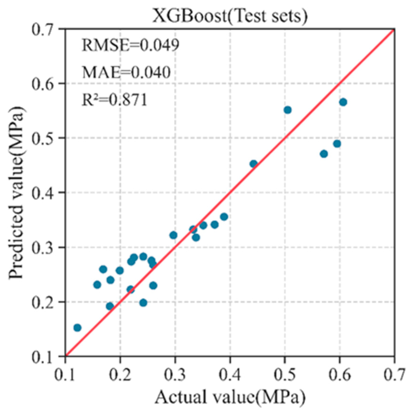
In the training set, a combination of the grid search method and the five-fold cross-validation method was used to optimize the parameters of the machine learning model. R2 was chosen as the main evaluation index to select the optimal combination of parameters, and the final evaluation result was the mean value of the five-fold cross-validation results. The optimal combination of parameters is learning_rate = 0.21; max_depth = 7; min_child_weight = 4; and n_estimators = 129. The prediction performance of the model after parameter optimization was verified on the test set, and the MAE of the XGBoost model on the test set was 0.040 The relationship between the predicted and true values of the XGBoost model on the test set is shown in Figure 12, from which it can be seen that the predicted values of most samples in the model are very close to the true values.
The XGBoost model was compared with other traditional machine learning models. The models were evaluated using three metrics, MAE, RMSE, and R2, and a grid search combined with cross-validation was used for each model to optimize its parameters. Table 5 shows the prediction results of each traditional machine learning model on the test set, and it can be seen that the XGBoost model shows a good performance. The XGBoost model was compared with the KNN model, and the RMSE was reduced by 37%, the MAE was reduced by 38%, and the R2 was improved by 33%. The XGBoost model was compared with the SVM model, and the RMSE was reduced by 47%, the MAE was reduced by 47%, and the R2 was improved by 62%.
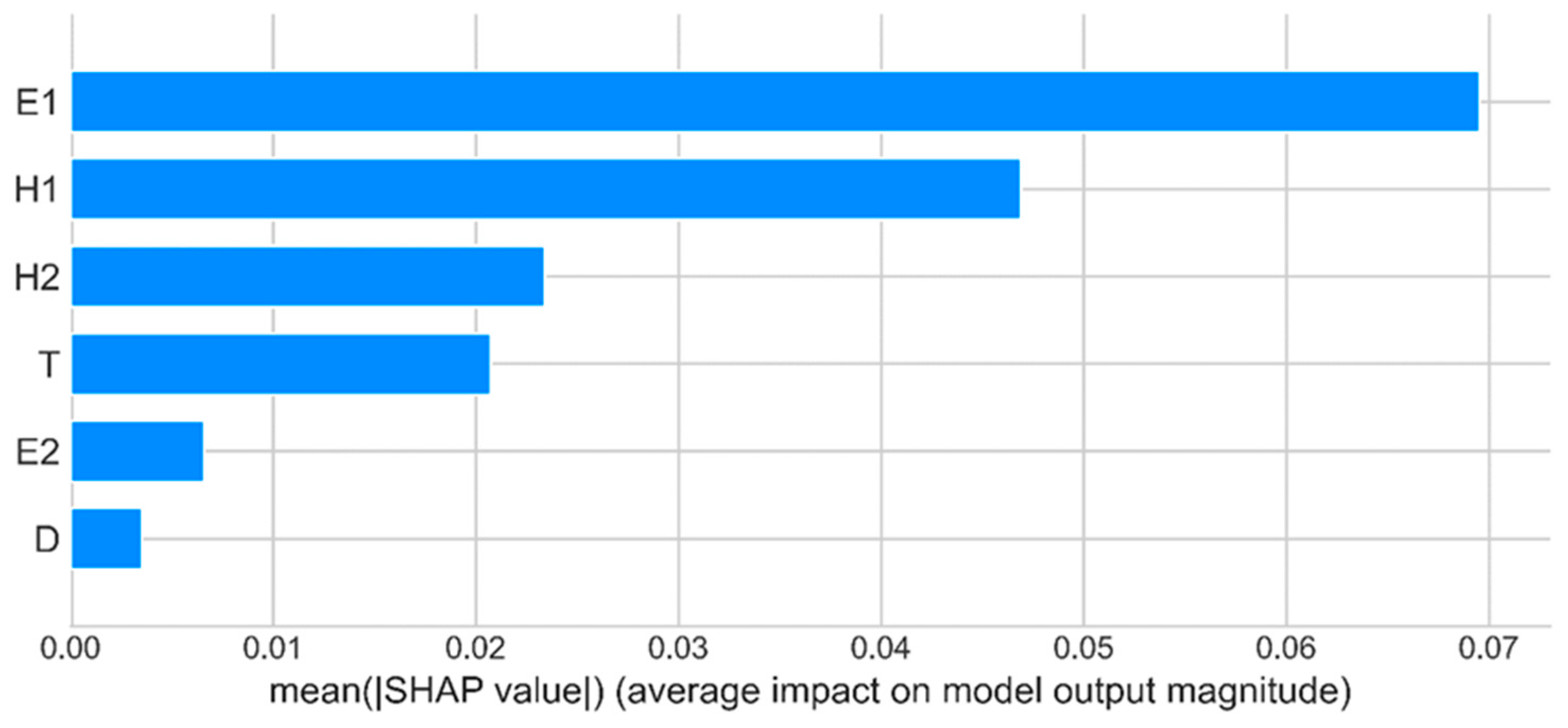
The SHAP architecture was used to perform an interpretability analysis of the developed prediction model, and the importance of the input feature variables is shown in Figure 13, where the importance of the input feature is calculated based on the average absolute value of each feature SHAP value. It can be seen from the figure that the most important feature variables are the upper pavement modulus of elasticity E1 and the upper pavement thickness H1, and the relatively more important feature variables are the lower pavement thickness H2 and the steel bridge panel thickness T.

5.2. Prediction Model for Maximum Longitudinal Tensile Stress on the Pavement Surface

In the training set, a combination of grid search and five-fold cross-validation was used to optimize the parameters of the machine learning model, and R2 was chosen as the main evaluation index to select the optimal combination of parameters, and the final evaluation result was the mean value of the five-fold cross-validation results. The optimal combination of parameters is learning_rate = 0.09; max_depth = 2; min_child_weight = 4; and n_estimators = 276. The prediction performance of the model after parameter optimization was verified on the test set. The relationship between the predicted and true values of the XGBoost model on the test set is shown in Figure 14, from which it can be seen that the predicted values of most samples in the model are very close to the true values.
The XGBoost model was compared with other traditional machine learning models. The models were evaluated using three metrics, MAE, RMSE, and R2, and a grid search combined with cross-validation was used for each model to optimize its parameters. Table 6 shows the prediction results of each traditional machine learning model on the test set, and it can be seen that the XGBoost model exhibits good performance. The XGBoost model was compared with the KNN model, and the RMSE was reduced by 43%, the MAE was reduced by 50%, and the R2 was improved by 9%. The XGBoost model was compared with the SVM model, and the RMSE was reduced by 71%, the MAE was reduced by 74%, and the R2 was improved by 61%.
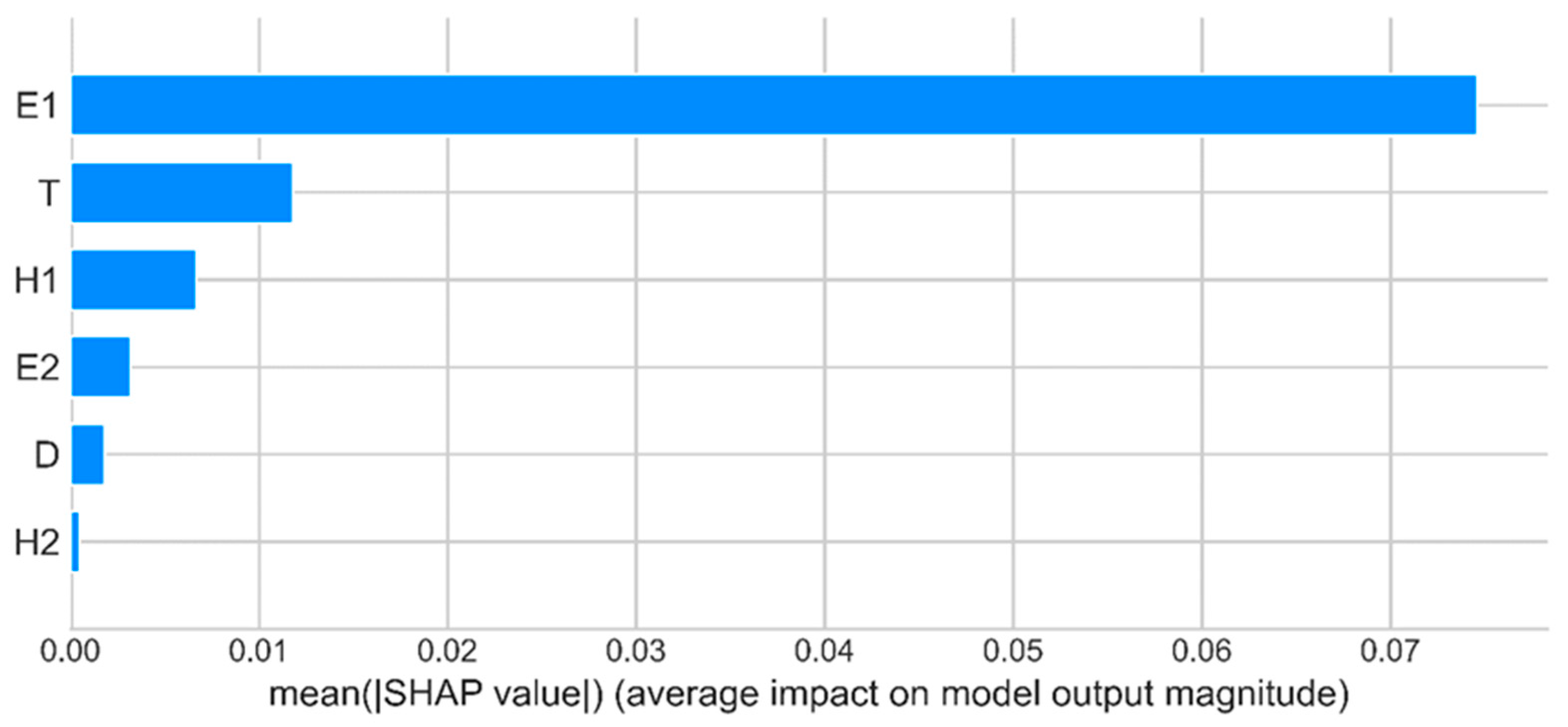
The importance of the input feature variables for the interpretability analysis of the developed prediction model using the SHAP architecture is shown in Figure 15. The most important characteristic variable is the modulus of elasticity of the upper layer of pavement E1, and the relatively more important characteristic variables are the thickness of the steel bridge panel T and the thickness of the upper layer of pavement H1.

5.3. Prediction Model for Maximum Transverse Shear Stress between Paving Layer and Steel Bridge Panel

In the training set, a combination of the grid search method and the five-fold cross-validation method was used to optimize the parameters of the machine learning model. R2 was chosen as the main evaluation index to select the optimal combination of parameters, and the final evaluation result was the mean value of the five-fold cross-validation results. The optimal combination of parameters is learning_rate = 0.4; max_depth = 9; min_child_weight = 3; and n_estimators = 170. The prediction performance of the optimized model was verified on the test set, and the MAE of the XGBoost model on the test set was 0.023 and the RMSE was 0.027. The relationship between the predicted and true values of the XGBoost model on the test set is shown in Figure 16, from which it can be seen that the predicted values of most of the samples in the model are very close to the true values.
The XGBoost model was compared with other traditional machine learning models. The models were evaluated using three metrics, MAE, RMSE, and R2, and a grid search combined with cross-validation was used for each model to optimize its parameters. Table 7 shows the prediction results of each traditional machine learning model on the test set, and it can be seen that the XGBoost model exhibits good performance. The XGBoost model was compared with the KNN model, and the RMSE was reduced by 28%, the MAE was reduced by 27%, and the R2 was improved by 10%. The XGBoost model was compared with the SVM model, and the RMSE was reduced by 44%, the MAE was reduced by 47%, and the R2 was improved by 46%.
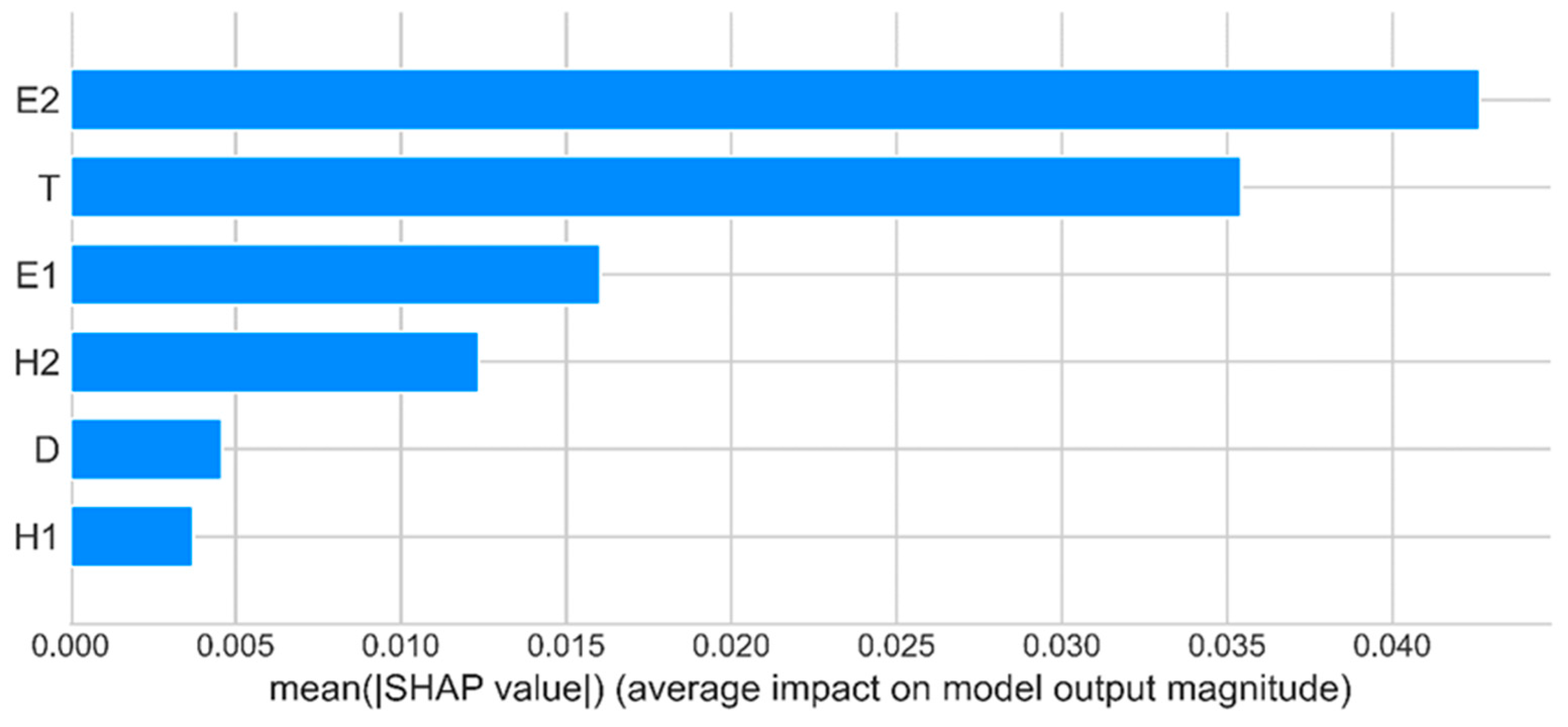
The importance of the input feature variables for the interpretability analysis of the developed prediction model using the SHAP architecture is shown in Figure 17. It can be seen from the figure that the most important characteristic variables are the lower pavement elastic modulus E2 and the steel bridge panel thickness T. The relatively more important characteristic variables are the upper pavement elastic modulus E1 and the lower pavement thickness H2.

5.4. Prediction Model for Maximum Longitudinal Shear Stress between Paving Layer and Steel Bridge Panel

In the training set, a combination of the grid search method and the five-fold cross-validation method was used to optimize the parameters of the machine learning model. R2 was chosen as the main evaluation index to select the optimal combination of parameters, and the final evaluation result was the mean value of the five-fold cross-validation results. The optimal combination of parameters is learning_rate = 0.15; max_depth = 10; min_child_weight = 4; and n_estimators = 230. The prediction performance of the model after parameter optimization was verified on the test set. The relationship between the predicted and true values of the XGBoost model on the test set is shown in Figure 18, from which it can be seen that the predicted values of most samples in the model are very close to the true values.
The XGBoost model is compared with other traditional machine learning models. The models were evaluated using three metrics, MAE, RMSE, and R2, and a grid search combined with cross-validation was used for each model to optimize its parameters. Table 8 shows the prediction results of each traditional machine learning model on the test set, and it can be seen that the XGBoost model shows good performance. The XGBoost model was compared with the KNN model, and the RMSE was reduced by 42%, the MAE was reduced by 48%, and the R2 was improved by 37%. The XGBoost model was compared with the SVM model, and the RMSE was reduced by 45%, the MAE was reduced by 50%, and the R2 was improved by 47%.
The importance of the input feature variables for the interpretability analysis of the developed prediction model using the SHAP architecture is shown in Figure 19. It can be seen from the figure that the most important characteristic variables are the lower pavement elastic modulus E2, and the relatively more important characteristic variables are the upper pavement elastic modulus E1 and the steel bridge panel thickness T.

5.5. Prediction Model for Maximum Vertical Displacement of Pavement Layer

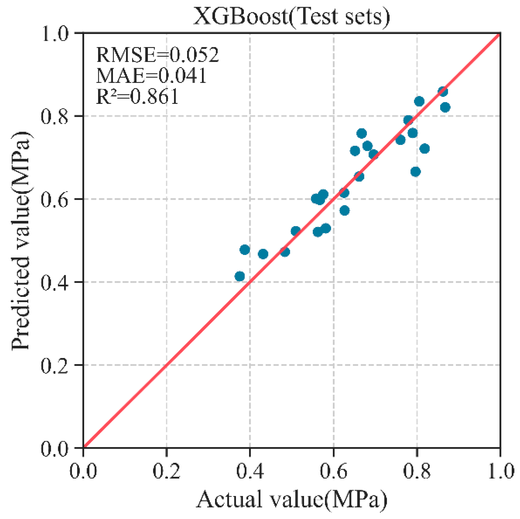
In the training set, a combination of the grid search method and the five-fold cross-validation method was used to optimize the parameters of the machine learning model. R2 was chosen as the main evaluation index to select the optimal combination of parameters, and the final evaluation result was the mean value of the five-fold cross-validation results. The optimal combination of parameters is learning_rate = 0.05; max_depth = 8; min_child_weight = 2; and n_estimators = 230. The prediction performance of the optimized model was verified on the test set, and the MAE of the XGBoost model on the test set was 0.041 The relationship between the predicted and true values of the XGBoost model on the test set is shown in Figure 20, from which it can be seen that the predicted values of most samples in the model are very close to the true values.
The XGBoost model was compared with other traditional machine learning models. The models were evaluated using three metrics, MAE, RMSE, and R2, and a grid search combined with cross-validation was used for each model to optimize its parameters. Table 9 shows the prediction results of each traditional machine learning model on the test set, and it can be seen that the XGBoost model shows good performance. The XGBoost model was compared with the KNN model, and the RMSE was reduced by 55%, the MAE was reduced by 52%, and the R2 was improved by 260%. The XGBoost model was compared with the SVM model, and the RMSE was reduced by 44%, the MAE was reduced by 39%, and the R2 was improved by 62%.
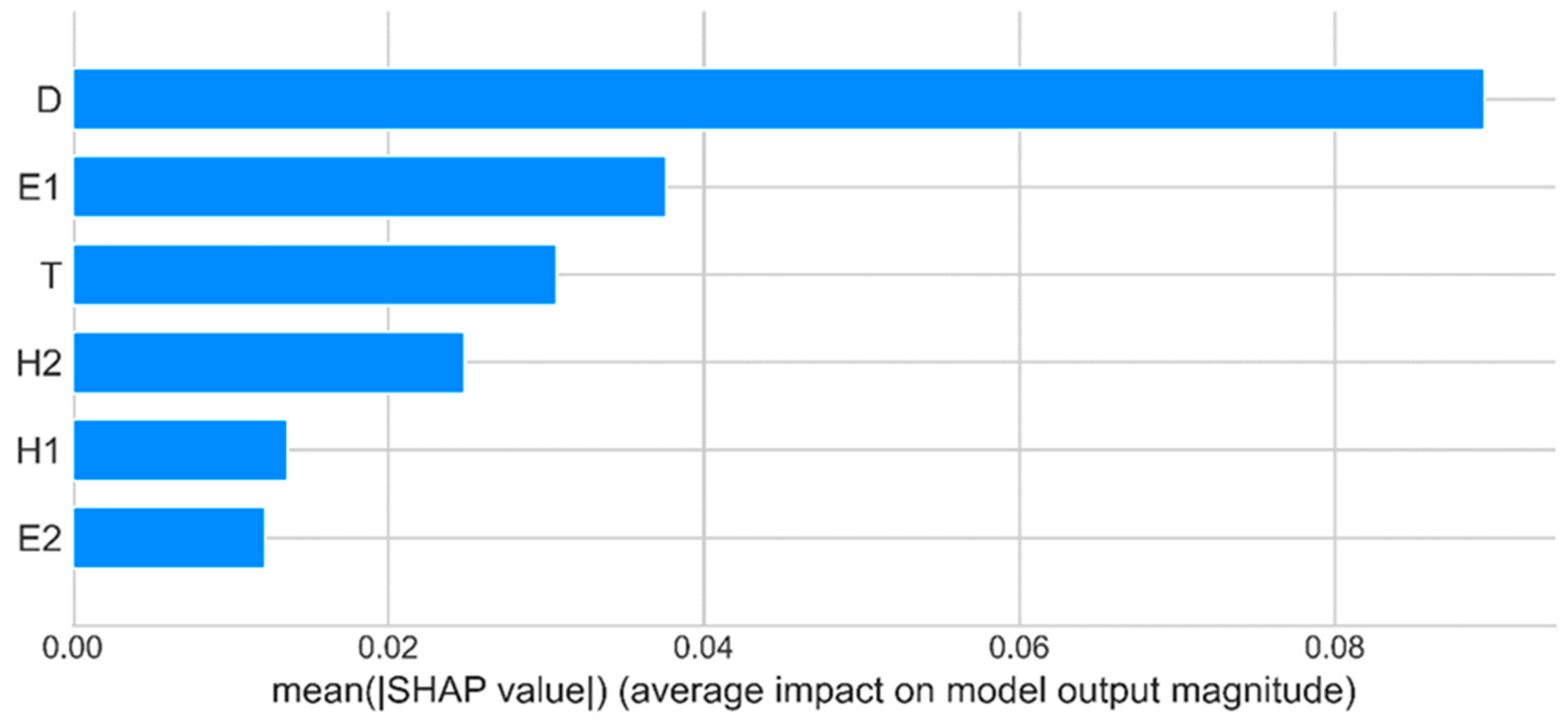
The importance of the input feature variables for the interpretability analysis of the developed prediction model using the SHAP architecture is shown in Figure 21. It can be seen from the figure that the most important feature variable is the spacing D of the diaphragm, and the relatively more important feature variables are the elastic modulus E1 of the upper layer of the pavement, the thickness T of the steel bridge panel, and the thickness H2 of the lower layer of the pavement.

6. Conclusions

This study developed an XGBoost-based mechanical performance prediction model for steel bridge deck pavement systems. The solution can be performed quickly and accurately. The dataset was established by conducting numerical simulation tests at the most unfavorable load locations using a finite element model. The XGBoost model was then built using the dataset, and its parameters were optimized. Next, the established XGBoost model was compared with other conventional machine learning models. Finally, the model was analyzed Interpretively using the SHAP framework. The following conclusions can be drawn from this study:
(1)
In the prediction model of the maximum transverse tensile stress on the pavement surface, the prediction results of the XGBoost model on the test set are as follows: MAE is 0.040, RMSE is 0.049, and R2 is 0.871. The optimal combination of parameters is learning_rate = 0.21; max_depth = 7; min_child_weight = 4; and n_estimators = 129. The most important characteristic variables are the elastic modulus of the upper layer of the pavement E1 and the thickness of the upper layer of the pavement H1, and the relatively more important characteristic variables are the thickness of the lower layer of the pavement H2 and the thickness of the steel bridge panel T.
(2)
In the prediction model of the maximum longitudinal tensile stress on the pavement surface, the prediction results of the XGBoost model on the test set are as follows: MAE is 0.013, RMSE is 0.015, and R2 is 0.970. The optimal combination of parameters is learning_rate = 0.09; max_depth = 2; min_child_weight = 4; and n_estimators = 276. The most important characteristic variables are the elastic modulus of the upper layer of the pavement E1, and the relatively more important characteristic variables are the thickness of the steel bridge panel T and the thickness of the upper layer of the pavement H1.
(3)
In the prediction model of the maximum transverse shear stress between the pavement and steel bridge panel, the prediction results of the XGBoost model on the test set are as follows: MAE is 0.023, RMSE is 0.027, and R2 is 0.864. The optimal combination of parameters is learning_rate = 0.4; max_depth = 9; min_child_weight = 3; and n_estimators = 170. The most important characteristic variables are the elastic modulus of lower pavement E2 and the thickness of steel bridge panel T. The relatively important characteristic variables are the elastic modulus of upper pavement E1 and the thickness of lower pavement H2.
(4)
In the prediction model of the maximum longitudinal shear stress between the pavement and steel bridge panel, the prediction results of the XGBoost model on the test set are as follows: MAE is 0.011, RMSE is 0.013, and R2 is 0.865. The optimal combination of parameters is learning_rate = 0.15; max_depth = 10; min_child_weight = 4; and n_estimators = 230. The most important characteristic variable is the elastic modulus of lower pavement E2, and the relatively more important characteristic variables are the elastic modulus of upper pavement E1 and the thickness of steel bridge panel T.
(5)
The prediction results of the XGBoost model on the test set in the maximum vertical displacement prediction model of the pavement layer are as follows: MAE is 0.041, RMSE is 0.052, and R2 is 0.861. The optimal combination of parameters is learning_rate = 0.05; max_depth = 8; min_child_weight = 2; and n_estimators = 230. The most important characteristic variable is the spacing of the cross-partition D, and the relatively more important characteristic variables are the elastic modulus of the upper layer of the pavement E1, the thickness of the steel bridge panel T, and the thickness of the lower layer of the pavement H2.
(6)
Compared with other traditional machine learning models, the XGBoost model shows a good prediction performance. Therefore, the XGBoost model developed in this study can be used as an accurate method to predict the mechanical properties of steel bridge deck pavement systems.
This study established only the mechanical performance index dataset under static load. The mechanical performance index dataset of the deck system under dynamic load should be established by a numerical simulation in future studies. The parameter optimization method used in this study for training the prediction model has a long running time and a large number of iterations. A more efficient parameter optimization method can be found in future studies.

Author Contributions

Y.W.: resources, writing—original draft, and writing—review and editing. R.J.: project administration and data curation. Q.L.: investigation and supervision. Z.S.: methodology, formal analysis, and software. All authors have read and agreed to the published version of the manuscript.

Funding

This research received no external funding.

Institutional Review Board Statement

Not applicable.

Informed Consent Statement

Not applicable.

Data Availability Statement

Data are contained within the article.

Conflicts of Interest

Authors Yazhou Wei and Rongqing Ji were employed by Henan Puwei Expressway Company Limited. The remaining authors declare that the research was conducted in the absence of any commercial or financial relationships that could be construed as a potential conflict of interest.

References

  1. Liu, Y.J.; Shen, Z.L.; Liu, J.; Chen, S.; Wang, J.P.; Wang, X.L. Advances in the application and research of steel bridge deck pavement. Structures 2022, 45, 1156–1174. [Google Scholar] [CrossRef]
  2. Xiu, L.; Zhou, C.J.; Qi, C.; Chen, L.L.; Feng, D.C. Experimental study on properties of epoxy binder and epoxy bonding chips layer for steel bridge deck pavement. Road Mater. Pavement Des. 2022, 23, 2451–2465. [Google Scholar]
  3. Liu, C.; Qian, Z.; Liao, Y.; Ren, H. A Comprehensive Life-Cycle Cost Analysis Approach Developed for Steel Bridge Deck Pavement Schemes. Coatings 2021, 11, 565. [Google Scholar] [CrossRef]
  4. Luo, S.; Qian, Z.; Yang, X.; Lu, Q. Laboratory evaluation of double-layered pavement structures for long-span steel bridge decks. J. Mater. Civ. Eng. 2018, 30, 04018111. [Google Scholar] [CrossRef]
  5. Hai, H.V.; Tuan, N.Q.; Tuan, T.A.; Ha, T.T.C.; Anh, D.T. Mechanical behavior of the asphalt wearing surface on an orthotropic steel bridge deck under cyclic loading. Case Stud. Constr. Mater. 2022, 16, e00836. [Google Scholar]
  6. Chen, X.; Huang, W.; Qian, Z.; Zhang, L. Design principle of deck pavements for long-span steel bridges with heavy-duty traffic in China. Road Mater. Pavement Des. 2017, 18 (Suppl. S3), 226–239. [Google Scholar] [CrossRef]
  7. Chen, X.; Qian, Z.; Liu, X.; Lei, Z. State of the art of asphalt surfacings on long-spanned orthotropic steel decks in China. J. Test. Eval. 2012, 40, 1252–1259. [Google Scholar] [CrossRef]
  8. Battista, R.; Pfeil, M. Fatigue Cracks Induced by Traffic Loading on Steel Bridges’ Slender Orthotropic Decks; WIT Transactions on Modelling and Simulation: Southampton, UK, 1999; Volume 22. [Google Scholar]
  9. Seim, C.; Ingham, T. Influence of wearing surfacing on performance of orthotropic steel plate decks. Transp. Res. Rec. 2004, 1892, 98–106. [Google Scholar] [CrossRef]
  10. Kim, T.W.; Baek, J.; Lee, H.J.; Lee, S.Y. Effect of pavement design parameters on the behaviour of orthotropic steel bridge deck pavements under traffic loading. Int. J. Pavement Eng. 2014, 15, 471–482. [Google Scholar] [CrossRef]
  11. Chen, L.; Qian, Z.; Wang, J. Multiscale numerical modeling of steel bridge deck pavements considering vehicle–pavement interaction. Int. J. Geomech. 2016, 16, B4015002. [Google Scholar] [CrossRef]
  12. Li, Q.; Song, Z. Prediction of compressive strength of rice husk ash concrete based on stacking ensemble learning model. J. Clean. Prod. 2023, 382, 135279. [Google Scholar] [CrossRef]
  13. Khalaj, G.; Nazari, A.; Pouraliakbar, H. Prediction of Martensite Fraction of Microalloyed Steel by Artificial Neural Networks. Neural Netw. World J. 2013, 23, 117–130. [Google Scholar] [CrossRef]
  14. Li, Q.-F.; Song, Z.-M. High-performance concrete strength prediction based on ensemble learning. Constr. Build. Mater. 2022, 324, 126694. [Google Scholar] [CrossRef]
  15. Li, Q.; Song, Z. Ensemble-learning-based prediction of steel bridge deck defect condition. Appl. Sci. 2022, 12, 5442. [Google Scholar] [CrossRef]
  16. Lyngdoh, G.A.; Zaki, M.; Krishnan, N.A.; Das, S. Prediction of concrete strengths enabled by missing data imputation and interpretable machine learning. Cem. Concr. Compos. 2022, 128, 104414. [Google Scholar] [CrossRef]
  17. Nguyen-Sy, T.; Wakim, J.; To, Q.-D.; Vu, M.-N.; Nguyen, T.-D.; Nguyen, T.-T. Predicting the compressive strength of concrete from its compositions and age using the extreme gradient boosting method. Constr. Build. Mater. 2020, 260, 119757. [Google Scholar] [CrossRef]
  18. Liang, W.; Luo, S.; Zhao, G.; Wu, H. Predicting hard rock pillar stability using GBDT, XGBoost, and LightGBM algorithms. Mathematics 2020, 8, 765. [Google Scholar] [CrossRef]
  19. Feng, D.-C.; Wang, W.-J.; Mangalathu, S.; Hu, G.; Wu, T. Implementing ensemble learning methods to predict the shear strength of RC deep beams with/without web reinforcements. Eng. Struct. 2021, 235, 111979. [Google Scholar] [CrossRef]
  20. Bakouregui, A.S.; Mohamed, H.M.; Yahia, A.; Benmokrane, B. Explainable extreme gradient boosting tree-based prediction of load-carrying capacity of FRP-RC columns. Eng. Struct. 2021, 245, 112836. [Google Scholar] [CrossRef]
  21. Chen, W.; Zhang, L. Building vulnerability assessment in seismic areas using ensemble learning: A Nepal case study. J. Clean. Prod. 2022, 350, 131418. [Google Scholar] [CrossRef]
  22. Ali, G.; Amin, S.; Hadi, A.; Hossein, S. Situational awareness and deficiency warning system in a smart distribution network based on stacking ensemble learning. Appl. Soft Comput. J. 2022, 128, 109427. [Google Scholar]
  23. Zhou, Z.-H. Ensemble Methods: Foundations and Algorithms; CRC Press: Boca Raton, FL, USA, 2012. [Google Scholar]
  24. Chen, T.; Guestrin, C. Xgboost: A scalable tree boosting system. In Proceedings of the 22nd Acm Sigkdd International Conference on Knowledge Discovery and Data Mining, San Francisco, CA, USA, 13–17 August 2016; pp. 785–794. [Google Scholar]
  25. Lundberg, S.M.; Lee, S.-I. A unified approach to interpreting model predictions. Adv. Neural Inf. Process. Syst. 2017, 30. [Google Scholar]
  26. Anas, A.A.; Mudassir, I.; Muhammad, Z.; Kaffayatullah, K.; Muhammad, N.A.; Jalal, F.E. Prediction of rapid chloride penetration resistance of metakaolin based high strength concrete using light GBM and XGBoost models by incorporating SHAP analysis. Constr. Build. Mater. 2022, 345, 128296. [Google Scholar]
  27. Ji, S.J.; Wang, X.; Tao, L.; Liu, X.J.; Wang, Y.Q.; Eva, H.; Sun, Z.W. Understanding cycling distance according to the prediction of the XGBoost and the interpretation of SHAP: A non-linear and interaction effect analysis. J. Transp. Geogr. 2022, 103, 103414. [Google Scholar] [CrossRef]
  28. JTG D64-2015; Code for Design of Highway Steel Structure Bridges. National Standards of the People’s Republic of China: Beijing, China, 2015.
  29. JTG/T 3364-02-2019; Specifications for Design and Construction of Pavement on Highway Steel Deck Bridge. National Standards of the People’s Republic of China: Beijing, China, 2019.
  30. Zhang, C.; Liu, C.; Zhang, X.; Almpanidis, G. An up-to-date comparison of state-of-the-art classification algorithms. Expert Syst. Appl. 2017, 82, 128–150. [Google Scholar] [CrossRef]
  31. Pedregosa, F.; Varoquaux, G.; Gramfort, A.; Michel, V.; Thirion, B.; Grisel, O.; Blondel, M.; Prettenhofer, P.; Weiss, R.; Dubourg, V.; et al. Scikit-learn: Machine Learning in Python. J. Mach. Learn. Res. 2011, 12, 2825–2830. [Google Scholar]
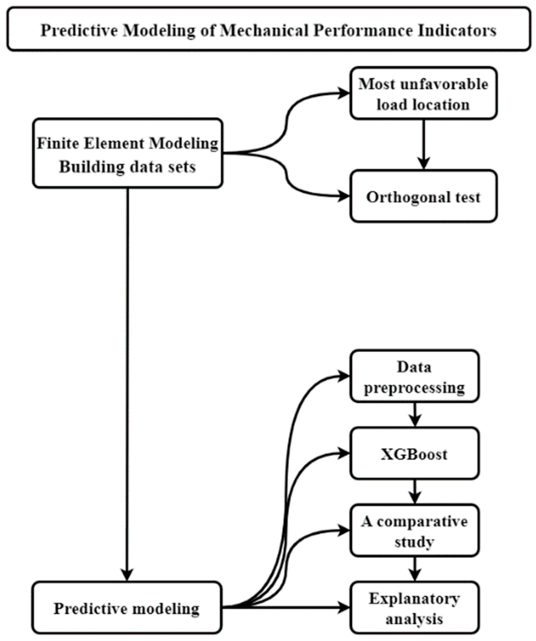
Figure 1. Technical route.
Applsci 13 12048 g001
Figure 2. The standard cross-section of a steel box girder.
Applsci 13 12048 g002
Figure 3. Load equivalent effect.
Applsci 13 12048 g003
Figure 4. Finite element model.
Applsci 13 12048 g004
Figure 5. Transverse load level.
Applsci 13 12048 g005
Figure 6. Longitudinal load level.
Applsci 13 12048 g006
Figure 7. Maximum transverse tensile stress on the surface of the pavement.
Applsci 13 12048 g007
Figure 8. Maximum longitudinal tensile stress on the surface of the pavement.
Applsci 13 12048 g008
Figure 9. Maximum transverse shear stress between paving layer and steel bridge panel.
Applsci 13 12048 g009
Figure 10. Maximum longitudinal shear stress between the pavement and the steel bridge deck.
Applsci 13 12048 g010
Figure 11. Maximum vertical displacement of pavement layer.
Applsci 13 12048 g011
Figure 12. Relationship between predicted and true values of XGBoost model on the test set. Line: predicted values, points: true values.
Applsci 13 12048 g012
Figure 13. Importance of input feature variables.
Applsci 13 12048 g013
Figure 14. Relationship between predicted and true values of XGBoost model on the test set. Line: predicted values, points: true values.
Applsci 13 12048 g014
Figure 15. Importance of input feature variables.
Applsci 13 12048 g015
Figure 16. Relationship between predicted and true values of XGBoost model on the test set. Line: predicted values, points: true values.
Applsci 13 12048 g016
Figure 17. Importance of input feature variables.
Applsci 13 12048 g017
Figure 18. Relationship between predicted and true values of XGBoost model on the test set. Line: predicted values, points: true values.
Applsci 13 12048 g018
Figure 19. Importance of input feature variables.
Applsci 13 12048 g019
Figure 20. Relationship between predicted and true values of XGBoost model on the test set. Line: predicted values, points: true values.
Applsci 13 12048 g020
Figure 21. Importance of input feature variables.
Applsci 13 12048 g021
Table 1. Finite element model parameters.
Model ParametersValuesModel ParametersValues
Thickness of upper layer of pavement30 mmU-shape stiffening rib
spacing
600 mm
Thickness of lower layer of pavement30 mmHeight of U-shaped
stiffening ribs
280 mm
Modulus of elasticity of upper
pavement layer
6800 MPaWidth of upper opening of U-shaped stiffening rib300 mm
Modulus of elasticity of lower
pavement layer
6800 MPaWidth of lower opening of U-shaped stiffening rib170 mm
Poisson’s ratio of upper
pavement layer
0.35Thickness of U-shaped
stiffening ribs
8 mm
Poisson’s ratio of lower
pavement layer
0.35Spacing of horizontal spacer3000 mm
Thickness of steel bridge panel16 mmThickness of horizontal spacer12 mm
Modulus of elasticity of steel bridge panel206,000 MPaHeight of horizontal spacer1000 mm
Poisson’s ratio of steel bridge panel0.3
Table 2. Calculation results of mechanical performance index.
Transverse Load LevelLongitudinal Load Level
Distance (mm)
A1
(MPa)
A2
(MPa)
B1
(MPa)
B2
(MPa)
C
(mm)
Load position one00.1110.0560.0860.0510.049
3000.2110.3350.1630.1210.138
6000.3090.3560.2180.1320.255
9000.3570.3500.2540.1420.357
12000.3720.3150.2740.1510.423
15000.3780.2710.2800.1730.449
Load position two00.3070.1560.3990.1550.072
3000.3020.3500.4080.2040.141
6000.3080.3450.4040.2100.252
9000.3240.3390.4160.2160.352
12000.3510.3050.4200.2230.418
15000.3570.2630.4230.2300.440
Load position three00.1410.0810.0860.0590.056
3000.2120.2720.1660.1290.138
6000.2340.2990.1920.1390.246
9000.2650.2990.2000.1470.339
12000.3010.2720.1990.1540.401
15000.3110.2390.1980.1730.425
Table 3. Influencing factors and level taking of the test.
LevelFactors
E1 (MPa)E2 (MPa)H1 (mm)H2 (mm)T (mm)D (mm)
1100010002020123000
2200020002525143500
3300030003030164000
440004000353518
550005000404020
6600060004545
770007000
880008000
910,00010,000
Table 4. Statistical analysis of characteristic variables.
VariablesData
Type
Variable TypeAverageStandard Deviation
Modulus of elasticity of the upper layer of pavement(E1)NumericalInput5111.1112783.882
Modulus of elasticity of lower pavement layer(E2)NumericalInput5111.1112783.882
Thickness of upper pavement layer(H1)NumericalInput30.0008.216
Thickness of lower pavement layer(H2)NumericalInput30.0008.216
Thickness of steel bridge panel(T)NumericalInput15.5562.646
Transverse spacer spacing(D)NumericalInput3500.000410.792
Maximum transverse tensile stress on pavement surface(A1)NumericalOutput0.3190.128
The maximum longitudinal tensile stress on the surface of the pavement layer(A2)NumericalOutput0.2000.091
Maximum transverse shear stress between paving layer and steel bridge panel(B1)NumericalOutput0.3860.083
Maximum longitudinal shear stress between paving layer and steel bridge panel(B2)NumericalOutput0.1930.037
Maximum vertical displacement of pavement layer(C)NumericalOutput0.6300.140
Table 5. Comparison with other traditional machine learning models.
ModelMAERMSER2
XGBoost0.0400.0490.871
KNN0.0640.0800.657
SVM0.0760.0930.537
Table 6. Comparison with other traditional machine learning models.
ModelMAERMSER2
XGBoost0.0130.0150.970
KNN0.0230.0300.889
SVM0.0460.0570.601
Table 7. Comparison with other traditional machine learning models.
ModelMAERMSER2
XGBoost0.0230.0270.864
KNN0.0320.0370.783
SVM0.0410.0510.592
Table 8. Comparison with other traditional machine learning models.
ModelMAERMSER2
XGBoost0.0110.0130.865
KNN0.0190.0250.631
SVM0.0200.0260.590
Table 9. Comparison with other traditional machine learning models.
ModelMAERMSER2
XGBoost0.0410.0520.861
KNN0.0920.1090.239
SVM0.0730.0850.533
Disclaimer/Publisher’s Note: The statements, opinions and data contained in all publications are solely those of the individual author(s) and contributor(s) and not of MDPI and/or the editor(s). MDPI and/or the editor(s) disclaim responsibility for any injury to people or property resulting from any ideas, methods, instructions or products referred to in the content.