
Mechanical Performance Prediction Model of Steel Bridge Deck Pavement System Based on XGBoost

Abstract
:1. Introduction
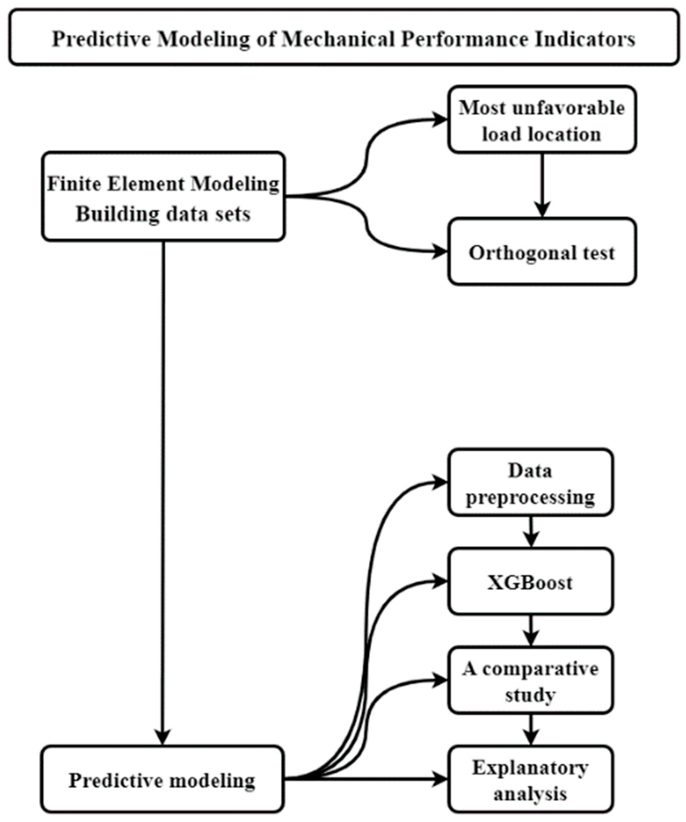
2. Method
2.1. XGBoost (Extreme Gradient Boosting)
2.2. SHAP (Shapley Additive Explanations)
3. Dataset Creation
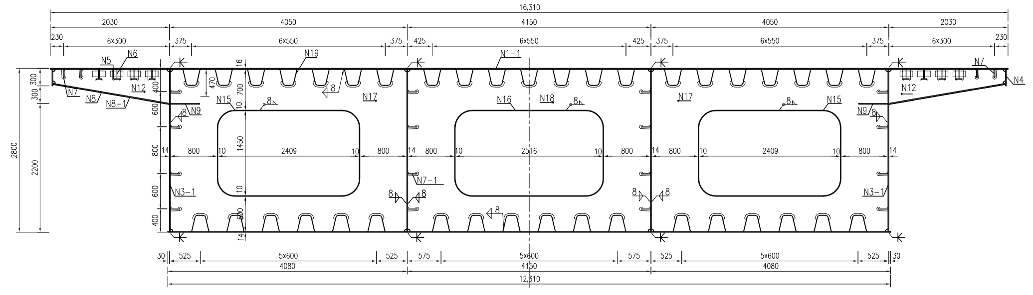
3.1. Finite Element Modeling
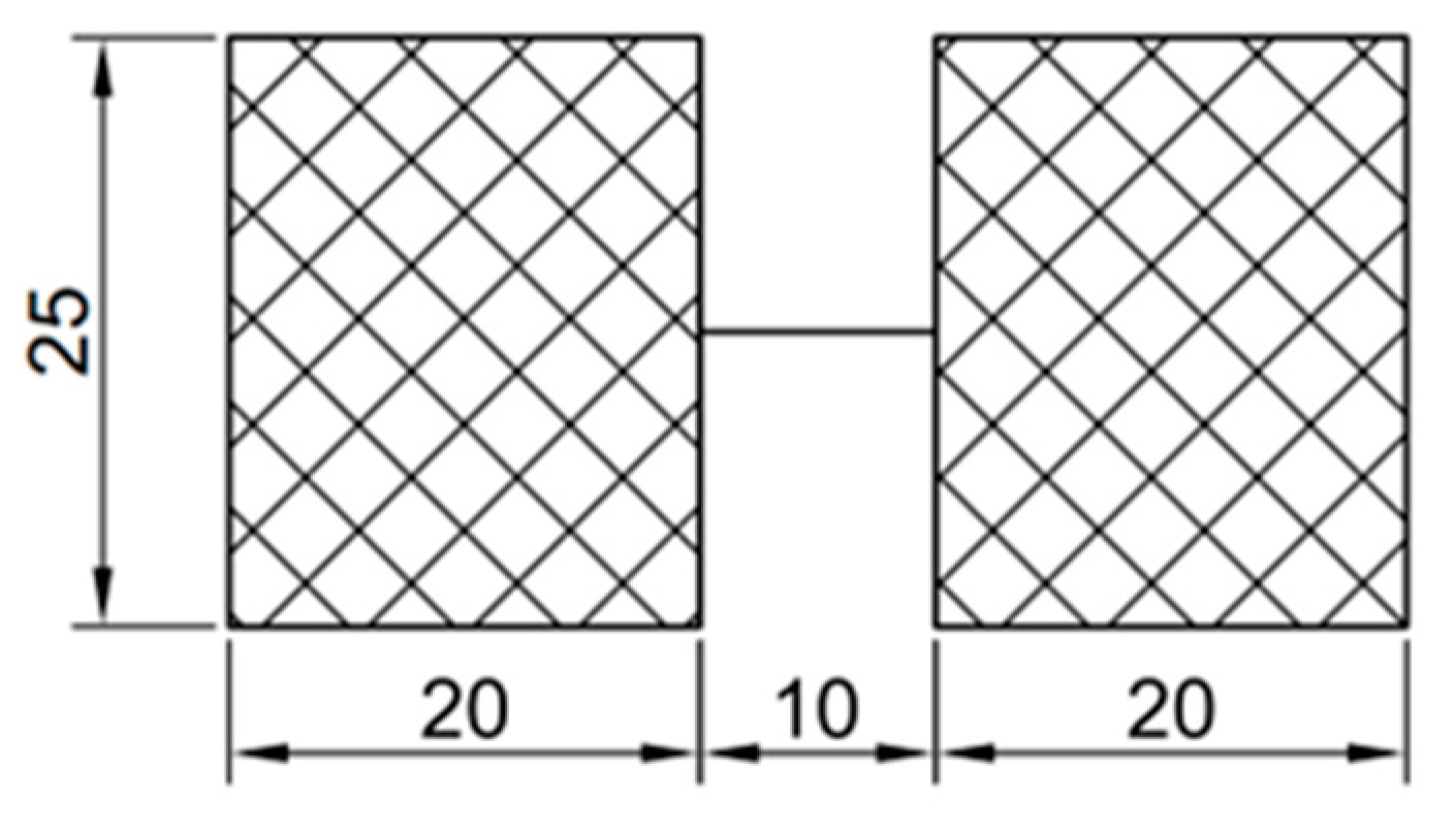
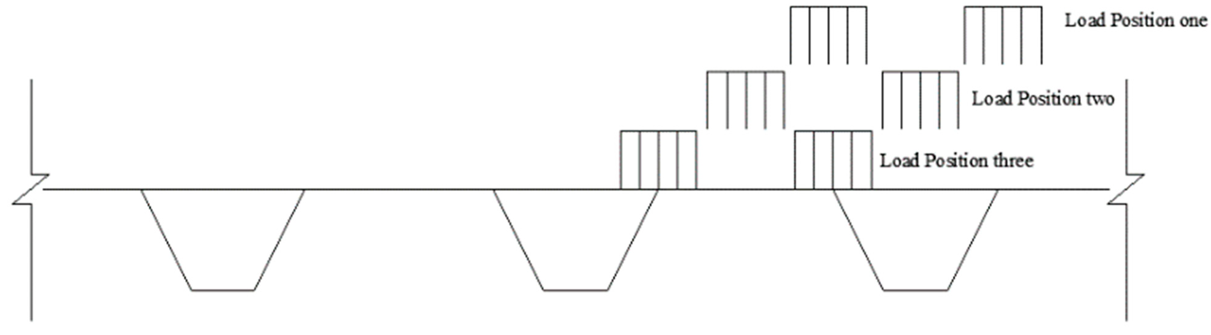
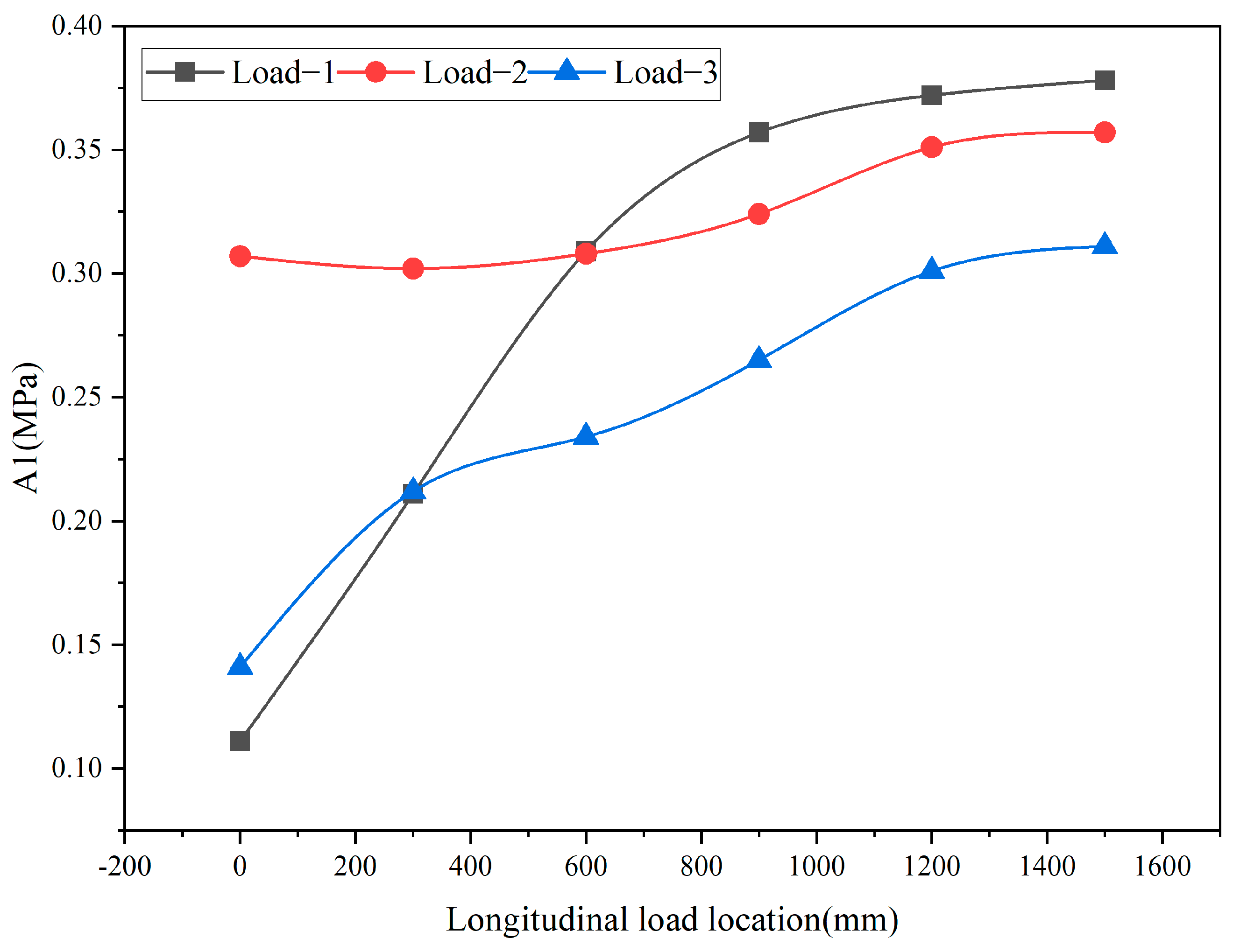
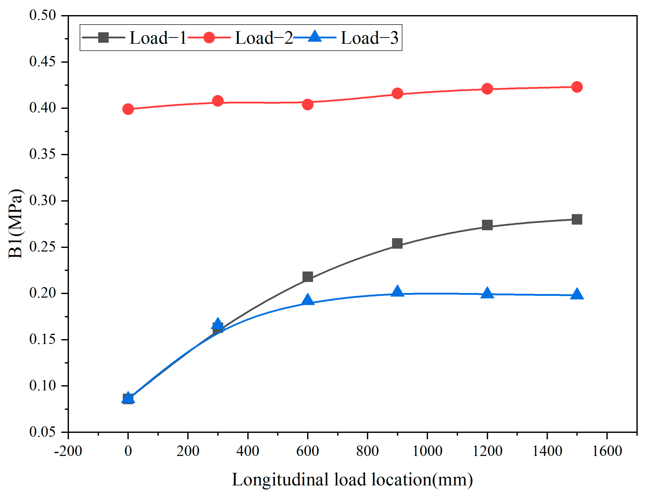
3.2. The Most Unfavorable Load Position
3.3. Orthogonal Test
4. Predictive Modeling
4.1. Data Preprocessing
4.2. Model Evaluation Metrics
5. Results and Discussion
5.1. Prediction Model for Maximum Transverse Tensile Stress on the Pavement Surface
5.2. Prediction Model for Maximum Longitudinal Tensile Stress on the Pavement Surface
5.3. Prediction Model for Maximum Transverse Shear Stress between Paving Layer and Steel Bridge Panel
5.4. Prediction Model for Maximum Longitudinal Shear Stress between Paving Layer and Steel Bridge Panel
5.5. Prediction Model for Maximum Vertical Displacement of Pavement Layer
6. Conclusions
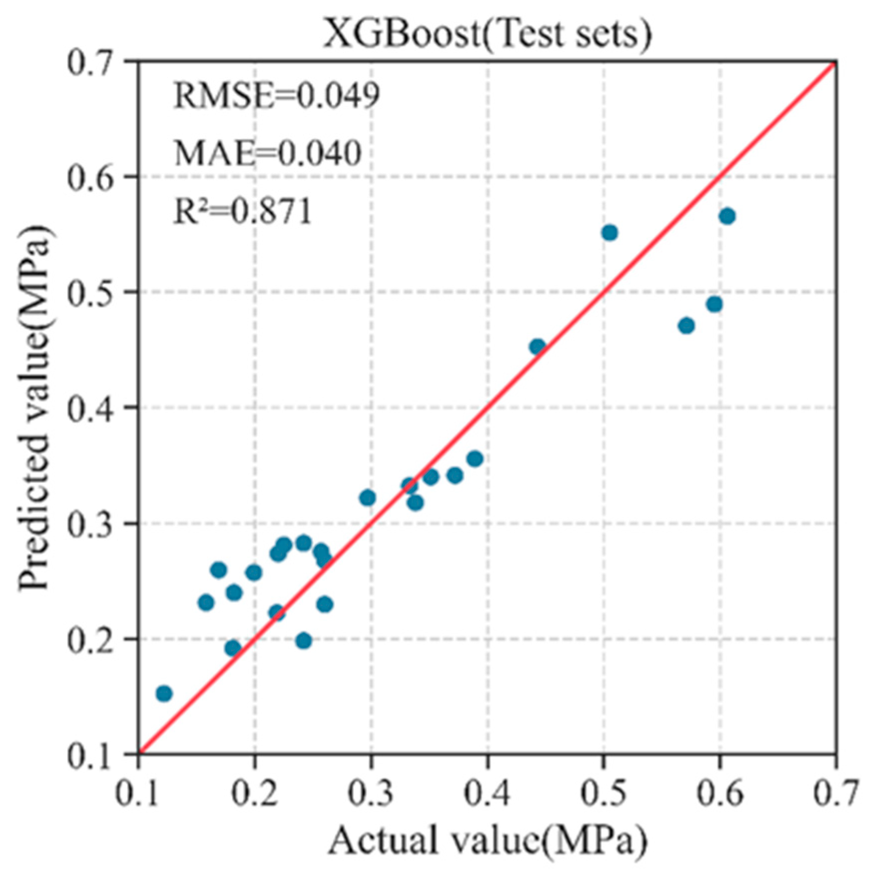
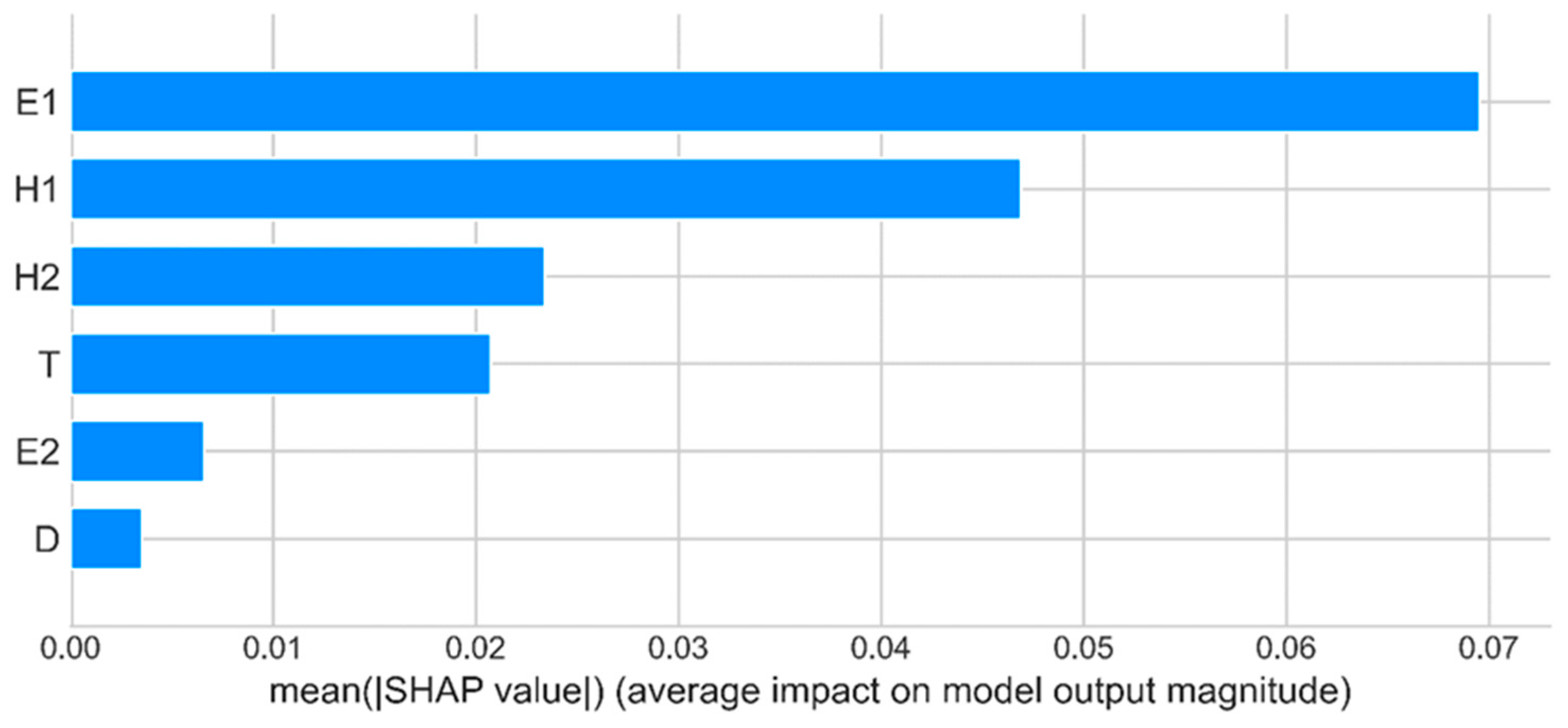
- (1)
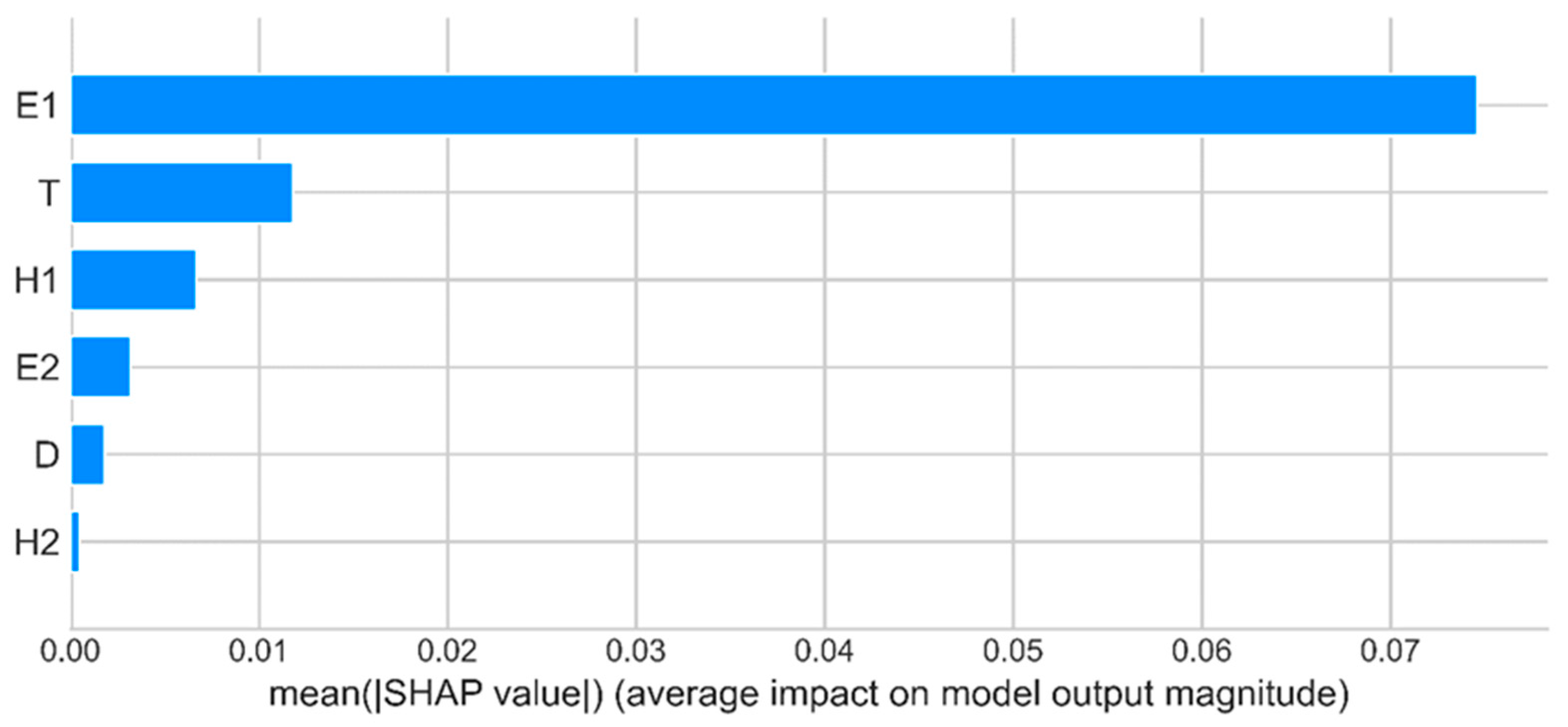
- In the prediction model of the maximum transverse tensile stress on the pavement surface, the prediction results of the XGBoost model on the test set are as follows: MAE is 0.040, RMSE is 0.049, and R2 is 0.871. The optimal combination of parameters is learning_rate = 0.21; max_depth = 7; min_child_weight = 4; and n_estimators = 129. The most important characteristic variables are the elastic modulus of the upper layer of the pavement E1 and the thickness of the upper layer of the pavement H1, and the relatively more important characteristic variables are the thickness of the lower layer of the pavement H2 and the thickness of the steel bridge panel T.
- (2)
- In the prediction model of the maximum longitudinal tensile stress on the pavement surface, the prediction results of the XGBoost model on the test set are as follows: MAE is 0.013, RMSE is 0.015, and R2 is 0.970. The optimal combination of parameters is learning_rate = 0.09; max_depth = 2; min_child_weight = 4; and n_estimators = 276. The most important characteristic variables are the elastic modulus of the upper layer of the pavement E1, and the relatively more important characteristic variables are the thickness of the steel bridge panel T and the thickness of the upper layer of the pavement H1.
- (3)
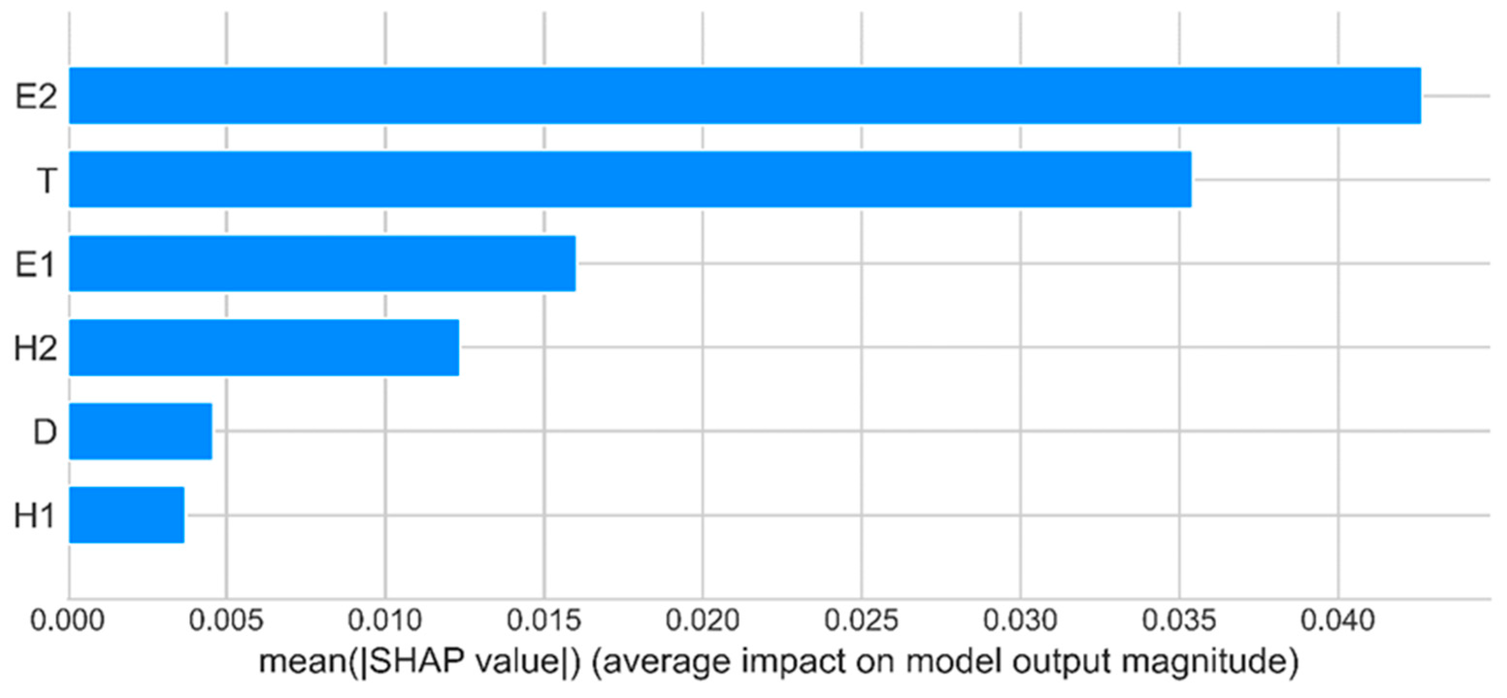
- In the prediction model of the maximum transverse shear stress between the pavement and steel bridge panel, the prediction results of the XGBoost model on the test set are as follows: MAE is 0.023, RMSE is 0.027, and R2 is 0.864. The optimal combination of parameters is learning_rate = 0.4; max_depth = 9; min_child_weight = 3; and n_estimators = 170. The most important characteristic variables are the elastic modulus of lower pavement E2 and the thickness of steel bridge panel T. The relatively important characteristic variables are the elastic modulus of upper pavement E1 and the thickness of lower pavement H2.
- (4)
- In the prediction model of the maximum longitudinal shear stress between the pavement and steel bridge panel, the prediction results of the XGBoost model on the test set are as follows: MAE is 0.011, RMSE is 0.013, and R2 is 0.865. The optimal combination of parameters is learning_rate = 0.15; max_depth = 10; min_child_weight = 4; and n_estimators = 230. The most important characteristic variable is the elastic modulus of lower pavement E2, and the relatively more important characteristic variables are the elastic modulus of upper pavement E1 and the thickness of steel bridge panel T.
- (5)
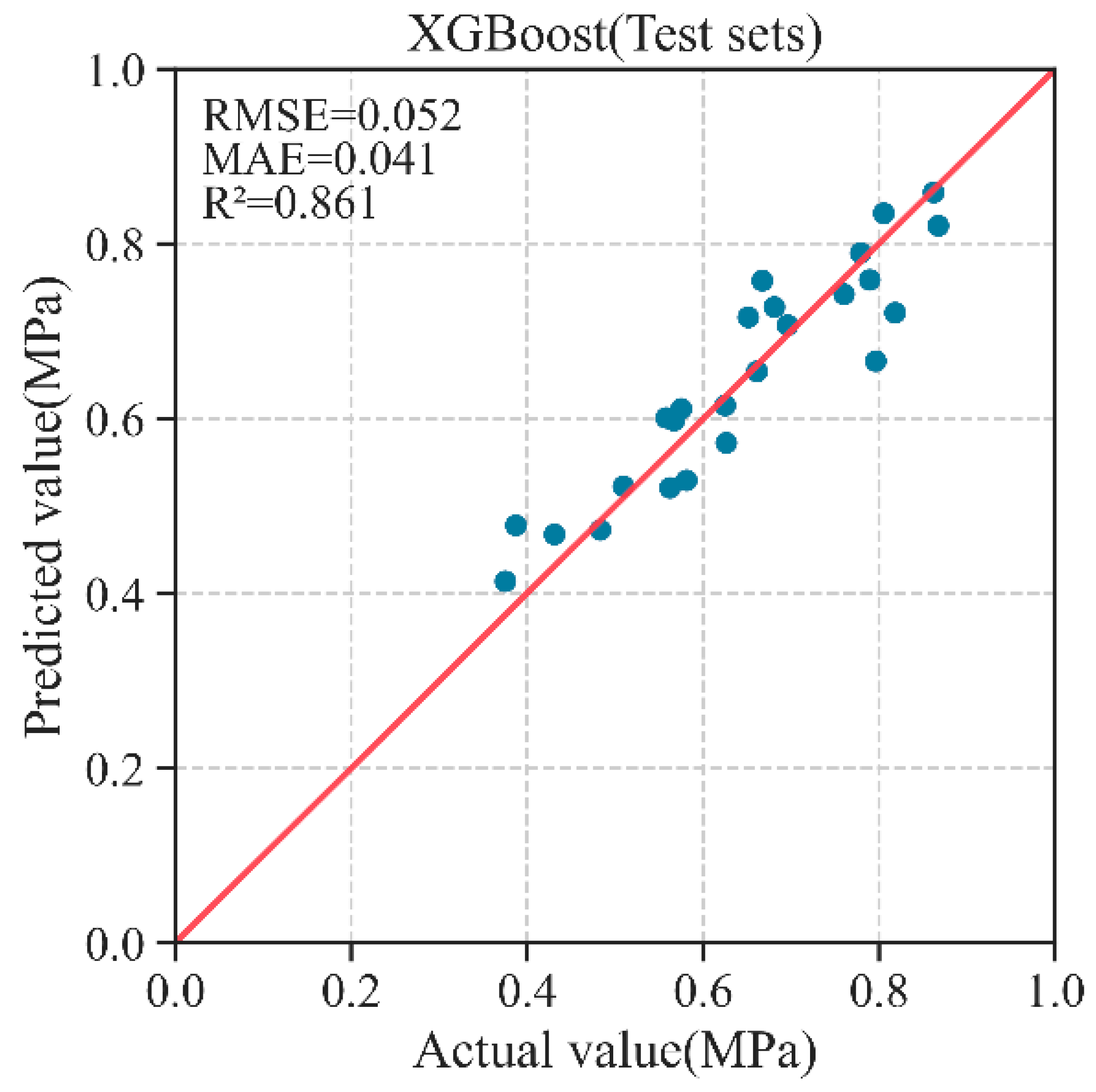
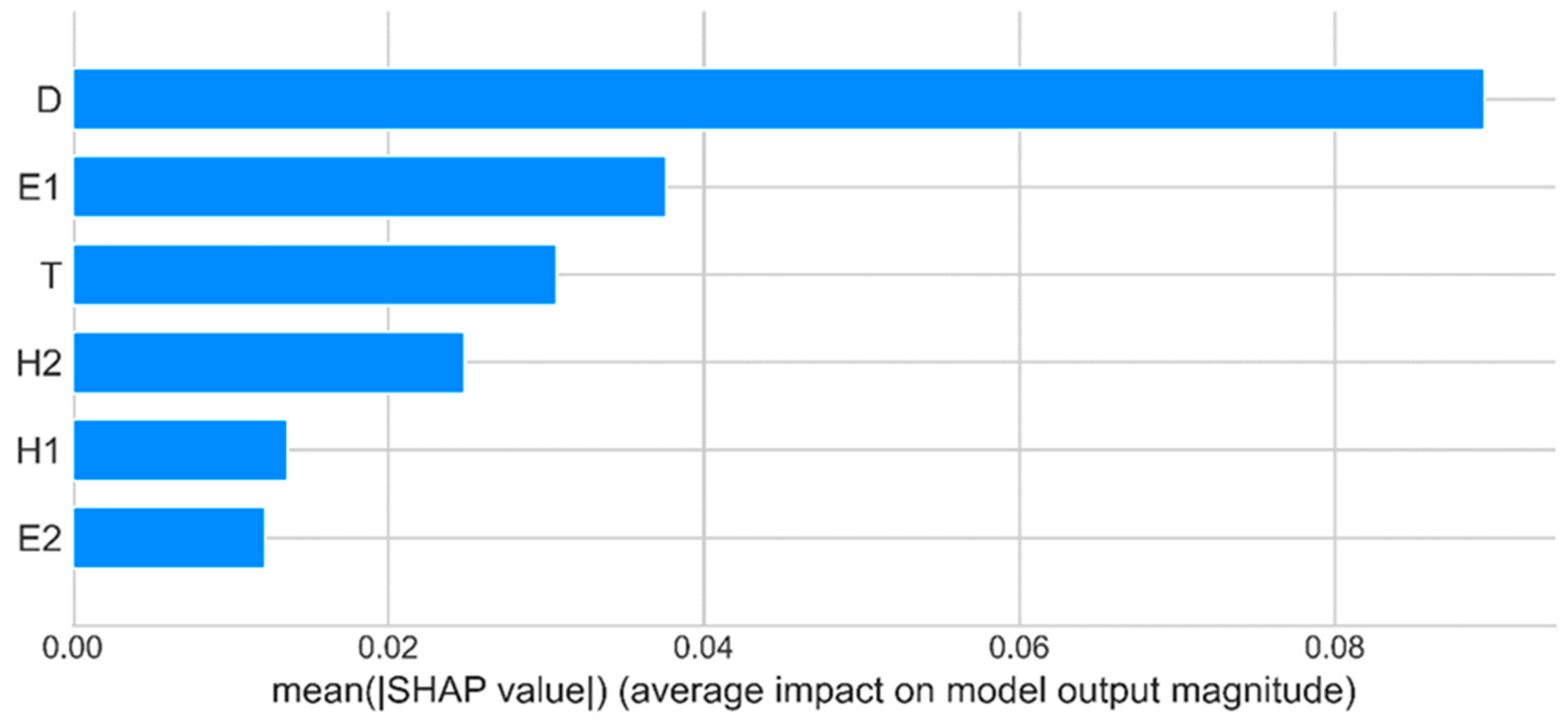
- The prediction results of the XGBoost model on the test set in the maximum vertical displacement prediction model of the pavement layer are as follows: MAE is 0.041, RMSE is 0.052, and R2 is 0.861. The optimal combination of parameters is learning_rate = 0.05; max_depth = 8; min_child_weight = 2; and n_estimators = 230. The most important characteristic variable is the spacing of the cross-partition D, and the relatively more important characteristic variables are the elastic modulus of the upper layer of the pavement E1, the thickness of the steel bridge panel T, and the thickness of the lower layer of the pavement H2.
- (6)
- Compared with other traditional machine learning models, the XGBoost model shows a good prediction performance. Therefore, the XGBoost model developed in this study can be used as an accurate method to predict the mechanical properties of steel bridge deck pavement systems.
Author Contributions
Funding
Institutional Review Board Statement
Informed Consent Statement
Data Availability Statement
Conflicts of Interest
References
- Liu, Y.J.; Shen, Z.L.; Liu, J.; Chen, S.; Wang, J.P.; Wang, X.L. Advances in the application and research of steel bridge deck pavement. Structures 2022, 45, 1156–1174. [Google Scholar] [CrossRef]
- Xiu, L.; Zhou, C.J.; Qi, C.; Chen, L.L.; Feng, D.C. Experimental study on properties of epoxy binder and epoxy bonding chips layer for steel bridge deck pavement. Road Mater. Pavement Des. 2022, 23, 2451–2465. [Google Scholar]
- Liu, C.; Qian, Z.; Liao, Y.; Ren, H. A Comprehensive Life-Cycle Cost Analysis Approach Developed for Steel Bridge Deck Pavement Schemes. Coatings 2021, 11, 565. [Google Scholar] [CrossRef]
- Luo, S.; Qian, Z.; Yang, X.; Lu, Q. Laboratory evaluation of double-layered pavement structures for long-span steel bridge decks. J. Mater. Civ. Eng. 2018, 30, 04018111. [Google Scholar] [CrossRef]
- Hai, H.V.; Tuan, N.Q.; Tuan, T.A.; Ha, T.T.C.; Anh, D.T. Mechanical behavior of the asphalt wearing surface on an orthotropic steel bridge deck under cyclic loading. Case Stud. Constr. Mater. 2022, 16, e00836. [Google Scholar]
- Chen, X.; Huang, W.; Qian, Z.; Zhang, L. Design principle of deck pavements for long-span steel bridges with heavy-duty traffic in China. Road Mater. Pavement Des. 2017, 18 (Suppl. S3), 226–239. [Google Scholar] [CrossRef]
- Chen, X.; Qian, Z.; Liu, X.; Lei, Z. State of the art of asphalt surfacings on long-spanned orthotropic steel decks in China. J. Test. Eval. 2012, 40, 1252–1259. [Google Scholar] [CrossRef]
- Battista, R.; Pfeil, M. Fatigue Cracks Induced by Traffic Loading on Steel Bridges’ Slender Orthotropic Decks; WIT Transactions on Modelling and Simulation: Southampton, UK, 1999; Volume 22. [Google Scholar]
- Seim, C.; Ingham, T. Influence of wearing surfacing on performance of orthotropic steel plate decks. Transp. Res. Rec. 2004, 1892, 98–106. [Google Scholar] [CrossRef]
- Kim, T.W.; Baek, J.; Lee, H.J.; Lee, S.Y. Effect of pavement design parameters on the behaviour of orthotropic steel bridge deck pavements under traffic loading. Int. J. Pavement Eng. 2014, 15, 471–482. [Google Scholar] [CrossRef]
- Chen, L.; Qian, Z.; Wang, J. Multiscale numerical modeling of steel bridge deck pavements considering vehicle–pavement interaction. Int. J. Geomech. 2016, 16, B4015002. [Google Scholar] [CrossRef]
- Li, Q.; Song, Z. Prediction of compressive strength of rice husk ash concrete based on stacking ensemble learning model. J. Clean. Prod. 2023, 382, 135279. [Google Scholar] [CrossRef]
- Khalaj, G.; Nazari, A.; Pouraliakbar, H. Prediction of Martensite Fraction of Microalloyed Steel by Artificial Neural Networks. Neural Netw. World J. 2013, 23, 117–130. [Google Scholar] [CrossRef]
- Li, Q.-F.; Song, Z.-M. High-performance concrete strength prediction based on ensemble learning. Constr. Build. Mater. 2022, 324, 126694. [Google Scholar] [CrossRef]
- Li, Q.; Song, Z. Ensemble-learning-based prediction of steel bridge deck defect condition. Appl. Sci. 2022, 12, 5442. [Google Scholar] [CrossRef]
- Lyngdoh, G.A.; Zaki, M.; Krishnan, N.A.; Das, S. Prediction of concrete strengths enabled by missing data imputation and interpretable machine learning. Cem. Concr. Compos. 2022, 128, 104414. [Google Scholar] [CrossRef]
- Nguyen-Sy, T.; Wakim, J.; To, Q.-D.; Vu, M.-N.; Nguyen, T.-D.; Nguyen, T.-T. Predicting the compressive strength of concrete from its compositions and age using the extreme gradient boosting method. Constr. Build. Mater. 2020, 260, 119757. [Google Scholar] [CrossRef]
- Liang, W.; Luo, S.; Zhao, G.; Wu, H. Predicting hard rock pillar stability using GBDT, XGBoost, and LightGBM algorithms. Mathematics 2020, 8, 765. [Google Scholar] [CrossRef]
- Feng, D.-C.; Wang, W.-J.; Mangalathu, S.; Hu, G.; Wu, T. Implementing ensemble learning methods to predict the shear strength of RC deep beams with/without web reinforcements. Eng. Struct. 2021, 235, 111979. [Google Scholar] [CrossRef]
- Bakouregui, A.S.; Mohamed, H.M.; Yahia, A.; Benmokrane, B. Explainable extreme gradient boosting tree-based prediction of load-carrying capacity of FRP-RC columns. Eng. Struct. 2021, 245, 112836. [Google Scholar] [CrossRef]
- Chen, W.; Zhang, L. Building vulnerability assessment in seismic areas using ensemble learning: A Nepal case study. J. Clean. Prod. 2022, 350, 131418. [Google Scholar] [CrossRef]
- Ali, G.; Amin, S.; Hadi, A.; Hossein, S. Situational awareness and deficiency warning system in a smart distribution network based on stacking ensemble learning. Appl. Soft Comput. J. 2022, 128, 109427. [Google Scholar]
- Zhou, Z.-H. Ensemble Methods: Foundations and Algorithms; CRC Press: Boca Raton, FL, USA, 2012. [Google Scholar]
- Chen, T.; Guestrin, C. Xgboost: A scalable tree boosting system. In Proceedings of the 22nd Acm Sigkdd International Conference on Knowledge Discovery and Data Mining, San Francisco, CA, USA, 13–17 August 2016; pp. 785–794. [Google Scholar]
- Lundberg, S.M.; Lee, S.-I. A unified approach to interpreting model predictions. Adv. Neural Inf. Process. Syst. 2017, 30. [Google Scholar]
- Anas, A.A.; Mudassir, I.; Muhammad, Z.; Kaffayatullah, K.; Muhammad, N.A.; Jalal, F.E. Prediction of rapid chloride penetration resistance of metakaolin based high strength concrete using light GBM and XGBoost models by incorporating SHAP analysis. Constr. Build. Mater. 2022, 345, 128296. [Google Scholar]
- Ji, S.J.; Wang, X.; Tao, L.; Liu, X.J.; Wang, Y.Q.; Eva, H.; Sun, Z.W. Understanding cycling distance according to the prediction of the XGBoost and the interpretation of SHAP: A non-linear and interaction effect analysis. J. Transp. Geogr. 2022, 103, 103414. [Google Scholar] [CrossRef]
- JTG D64-2015; Code for Design of Highway Steel Structure Bridges. National Standards of the People’s Republic of China: Beijing, China, 2015.
- JTG/T 3364-02-2019; Specifications for Design and Construction of Pavement on Highway Steel Deck Bridge. National Standards of the People’s Republic of China: Beijing, China, 2019.
- Zhang, C.; Liu, C.; Zhang, X.; Almpanidis, G. An up-to-date comparison of state-of-the-art classification algorithms. Expert Syst. Appl. 2017, 82, 128–150. [Google Scholar] [CrossRef]
- Pedregosa, F.; Varoquaux, G.; Gramfort, A.; Michel, V.; Thirion, B.; Grisel, O.; Blondel, M.; Prettenhofer, P.; Weiss, R.; Dubourg, V.; et al. Scikit-learn: Machine Learning in Python. J. Mach. Learn. Res. 2011, 12, 2825–2830. [Google Scholar]


| Model Parameters | Values | Model Parameters | Values |
|---|---|---|---|
| Thickness of upper layer of pavement | 30 mm | U-shape stiffening rib spacing | 600 mm |
| Thickness of lower layer of pavement | 30 mm | Height of U-shaped stiffening ribs | 280 mm |
| Modulus of elasticity of upper pavement layer | 6800 MPa | Width of upper opening of U-shaped stiffening rib | 300 mm |
| Modulus of elasticity of lower pavement layer | 6800 MPa | Width of lower opening of U-shaped stiffening rib | 170 mm |
| Poisson’s ratio of upper pavement layer | 0.35 | Thickness of U-shaped stiffening ribs | 8 mm |
| Poisson’s ratio of lower pavement layer | 0.35 | Spacing of horizontal spacer | 3000 mm |
| Thickness of steel bridge panel | 16 mm | Thickness of horizontal spacer | 12 mm |
| Modulus of elasticity of steel bridge panel | 206,000 MPa | Height of horizontal spacer | 1000 mm |
| Poisson’s ratio of steel bridge panel | 0.3 |
| Transverse Load Level | Longitudinal Load Level Distance (mm) | A1 (MPa) | A2 (MPa) | B1 (MPa) | B2 (MPa) | C (mm) |
|---|---|---|---|---|---|---|
| Load position one | 0 | 0.111 | 0.056 | 0.086 | 0.051 | 0.049 |
| 300 | 0.211 | 0.335 | 0.163 | 0.121 | 0.138 | |
| 600 | 0.309 | 0.356 | 0.218 | 0.132 | 0.255 | |
| 900 | 0.357 | 0.350 | 0.254 | 0.142 | 0.357 | |
| 1200 | 0.372 | 0.315 | 0.274 | 0.151 | 0.423 | |
| 1500 | 0.378 | 0.271 | 0.280 | 0.173 | 0.449 | |
| Load position two | 0 | 0.307 | 0.156 | 0.399 | 0.155 | 0.072 |
| 300 | 0.302 | 0.350 | 0.408 | 0.204 | 0.141 | |
| 600 | 0.308 | 0.345 | 0.404 | 0.210 | 0.252 | |
| 900 | 0.324 | 0.339 | 0.416 | 0.216 | 0.352 | |
| 1200 | 0.351 | 0.305 | 0.420 | 0.223 | 0.418 | |
| 1500 | 0.357 | 0.263 | 0.423 | 0.230 | 0.440 | |
| Load position three | 0 | 0.141 | 0.081 | 0.086 | 0.059 | 0.056 |
| 300 | 0.212 | 0.272 | 0.166 | 0.129 | 0.138 | |
| 600 | 0.234 | 0.299 | 0.192 | 0.139 | 0.246 | |
| 900 | 0.265 | 0.299 | 0.200 | 0.147 | 0.339 | |
| 1200 | 0.301 | 0.272 | 0.199 | 0.154 | 0.401 | |
| 1500 | 0.311 | 0.239 | 0.198 | 0.173 | 0.425 |
| Level | Factors | |||||
|---|---|---|---|---|---|---|
| E1 (MPa) | E2 (MPa) | H1 (mm) | H2 (mm) | T (mm) | D (mm) | |
| 1 | 1000 | 1000 | 20 | 20 | 12 | 3000 |
| 2 | 2000 | 2000 | 25 | 25 | 14 | 3500 |
| 3 | 3000 | 3000 | 30 | 30 | 16 | 4000 |
| 4 | 4000 | 4000 | 35 | 35 | 18 | |
| 5 | 5000 | 5000 | 40 | 40 | 20 | |
| 6 | 6000 | 6000 | 45 | 45 | ||
| 7 | 7000 | 7000 | ||||
| 8 | 8000 | 8000 | ||||
| 9 | 10,000 | 10,000 | ||||
| Variables | Data Type | Variable Type | Average | Standard Deviation |
|---|---|---|---|---|
| Modulus of elasticity of the upper layer of pavement(E1) | Numerical | Input | 5111.111 | 2783.882 |
| Modulus of elasticity of lower pavement layer(E2) | Numerical | Input | 5111.111 | 2783.882 |
| Thickness of upper pavement layer(H1) | Numerical | Input | 30.000 | 8.216 |
| Thickness of lower pavement layer(H2) | Numerical | Input | 30.000 | 8.216 |
| Thickness of steel bridge panel(T) | Numerical | Input | 15.556 | 2.646 |
| Transverse spacer spacing(D) | Numerical | Input | 3500.000 | 410.792 |
| Maximum transverse tensile stress on pavement surface(A1) | Numerical | Output | 0.319 | 0.128 |
| The maximum longitudinal tensile stress on the surface of the pavement layer(A2) | Numerical | Output | 0.200 | 0.091 |
| Maximum transverse shear stress between paving layer and steel bridge panel(B1) | Numerical | Output | 0.386 | 0.083 |
| Maximum longitudinal shear stress between paving layer and steel bridge panel(B2) | Numerical | Output | 0.193 | 0.037 |
| Maximum vertical displacement of pavement layer(C) | Numerical | Output | 0.630 | 0.140 |
| Model | MAE | RMSE | R2 |
|---|---|---|---|
| XGBoost | 0.040 | 0.049 | 0.871 |
| KNN | 0.064 | 0.080 | 0.657 |
| SVM | 0.076 | 0.093 | 0.537 |
| Model | MAE | RMSE | R2 |
|---|---|---|---|
| XGBoost | 0.013 | 0.015 | 0.970 |
| KNN | 0.023 | 0.030 | 0.889 |
| SVM | 0.046 | 0.057 | 0.601 |
| Model | MAE | RMSE | R2 |
|---|---|---|---|
| XGBoost | 0.023 | 0.027 | 0.864 |
| KNN | 0.032 | 0.037 | 0.783 |
| SVM | 0.041 | 0.051 | 0.592 |
| Model | MAE | RMSE | R2 |
|---|---|---|---|
| XGBoost | 0.011 | 0.013 | 0.865 |
| KNN | 0.019 | 0.025 | 0.631 |
| SVM | 0.020 | 0.026 | 0.590 |
| Model | MAE | RMSE | R2 |
|---|---|---|---|
| XGBoost | 0.041 | 0.052 | 0.861 |
| KNN | 0.092 | 0.109 | 0.239 |
| SVM | 0.073 | 0.085 | 0.533 |
Disclaimer/Publisher’s Note: The statements, opinions and data contained in all publications are solely those of the individual author(s) and contributor(s) and not of MDPI and/or the editor(s). MDPI and/or the editor(s) disclaim responsibility for any injury to people or property resulting from any ideas, methods, instructions or products referred to in the content. |
© 2023 by the authors. Licensee MDPI, Basel, Switzerland. This article is an open access article distributed under the terms and conditions of the Creative Commons Attribution (CC BY) license (https://creativecommons.org/licenses/by/4.0/).
Share and Cite
Wei, Y.; Ji, R.; Li, Q.; Song, Z. Mechanical Performance Prediction Model of Steel Bridge Deck Pavement System Based on XGBoost. Appl. Sci. 2023, 13, 12048. https://doi.org/10.3390/app132112048
Wei Y, Ji R, Li Q, Song Z. Mechanical Performance Prediction Model of Steel Bridge Deck Pavement System Based on XGBoost. Applied Sciences. 2023; 13(21):12048. https://doi.org/10.3390/app132112048
Chicago/Turabian StyleWei, Yazhou, Rongqing Ji, Qingfu Li, and Zongming Song. 2023. "Mechanical Performance Prediction Model of Steel Bridge Deck Pavement System Based on XGBoost" Applied Sciences 13, no. 21: 12048. https://doi.org/10.3390/app132112048