
Parametric Analysis of Nonlinear Oscillations of the “Rotor–Weakly Conductive Viscous Fluid–Foundation” System under the Action of a Magnetic Field


Abstract
:1. Introduction
2. Materials and Methods
3. Special Cases
4. Free Oscillations of System
5. Results and Discussion

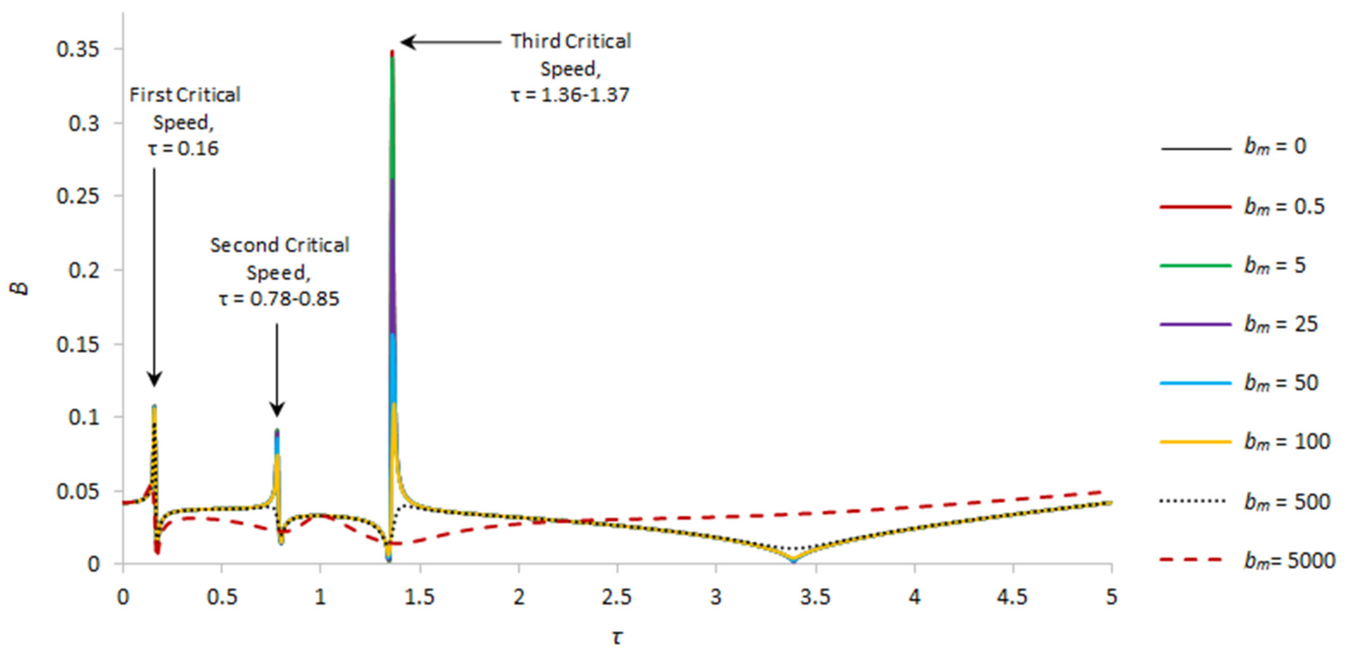
| B, γ = 13.8 | First Critical Speed Amplitude Value | Second Critical Speed Amplitude Value | Third Critical Speed Amplitude Value |
|---|---|---|---|
| bm = 0 | 0.1068045741, τ = 0.16 | 0.090720226, τ = 0.78 | 0.345717672, τ = 1.36 |
| bm = 0.5 | 0.106796702, τ = 0.16 | 0.090718, τ = 0.78 | 0.345709, τ = 1.36 |
| bm = 5 | 0.106725474, τ = 0.16 | 0.09065, τ = 0.78 | 0.341007, τ = 1.36 |
| bm = 25 | 0.10640083, τ = 0.16 | 0.089259, τ = 0.78 | 0.256448, τ = 1.36 |
| bm = 50 | 0.105976946, τ = 0.16 | 0.085366, τ = 0.78 | 0.155548, τ = 1.36 |
| bm = 100 | 0.105071989, τ = 0.16 | 0.073742909, τ = 0.78 | 0.109144682, τ = 1.36 |
| bm = 500 | 0.095853985, τ = 0.16 | 0.039189072, τ = 0.79 | 0.03976382, τ = 1.43 |
| bm = 5000 | 0.054819732, τ = 0.15 | 0.032983197, τ = 1 | – |
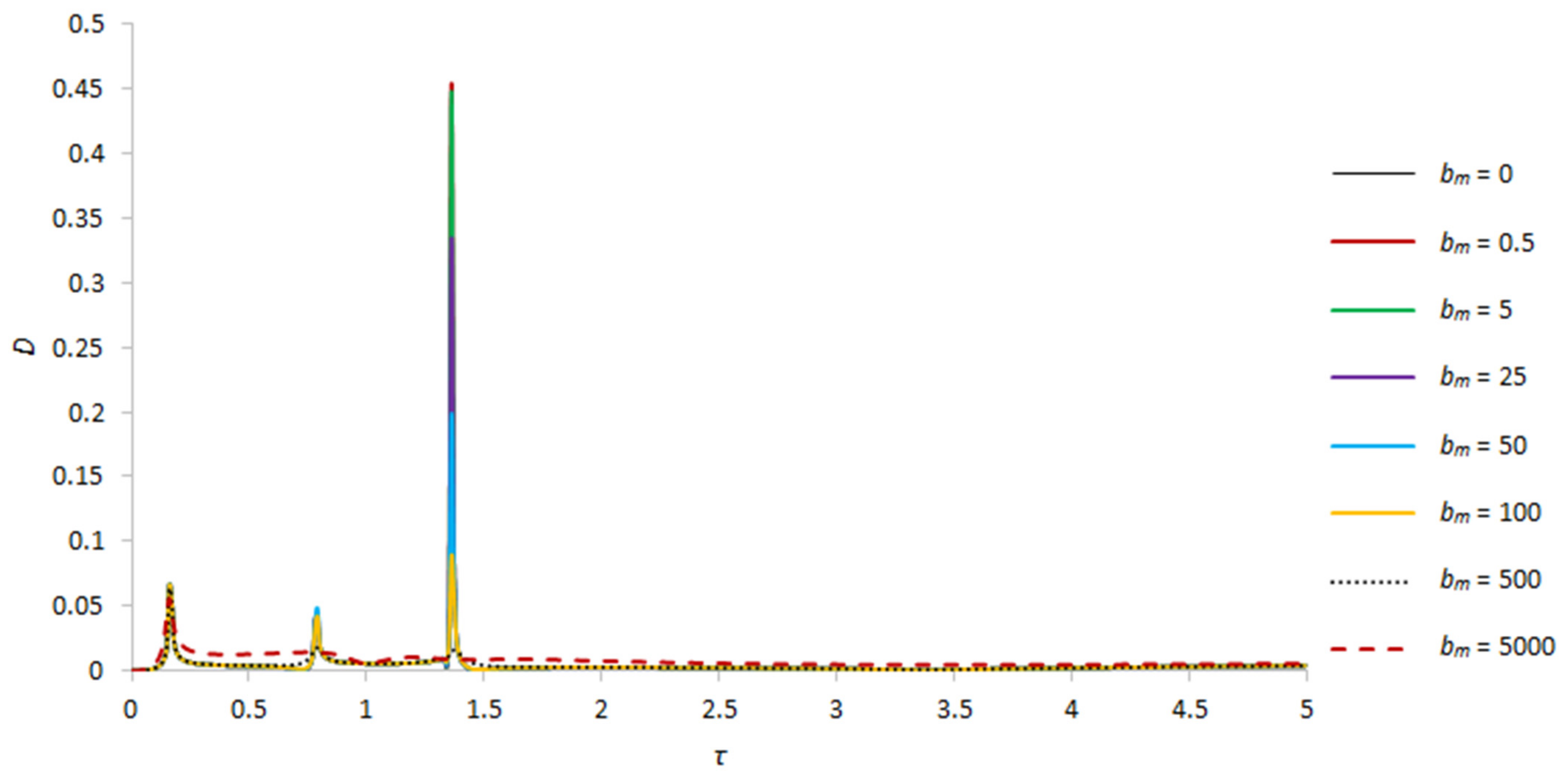
| D, γ = 13.8 | First Critical Speed Amplitude Value | Second Critical Speed Amplitude Value | Third Critical Speed Amplitude Value |
| bm = 0 | 0.066385927, τ = 0.16 | 0.040110122, τ = 0.78 | 0.453737506, τ = 1.36 |
| bm = 0.5 | 0.066382727, τ = 0.16 | 0.040109872, τ = 0.78 | 0.45372321, τ = 1.36 |
| bm = 5 | 0.066353881, τ = 0.16 | 0.040087202, τ = 0.78 | 0.447400839, τ = 1.36 |
| bm = 25 | 0.066224805, τ = 0.16 | 0.045069061, τ = 0.79 | 0.334005995, τ = 1.36 |
| bm = 50 | 0.066061617, τ = 0.16 | 0.048328381, τ = 0.79 | 0.198268343, τ = 1.36 |
| bm = 100 | 0.065730061, τ = 0.16 | 0.041947113, τ = 0.79 | 0.088761642, τ = 1.36 |
| bm = 500 | 0.063037959, τ = 0.16 | 0.01798351, τ = 0.79 | 0.016219871, τ = 1.37 |
| bm = 5000 | 0.054819732, τ = 0.16 | 0.014450226, τ = 0.85 | – |
| B, γ = 4.56 | First Critical Speed Amplitude Value | Second Critical Speed Amplitude Value | Third Critical Speed Amplitude Value |
|---|---|---|---|
| bm = 0 | 0.110805396, τ = 0.16 | 0.292896271, τ = 0.69 | 1.917205238, τ = 1.76 |
| bm = 0.5 | 0.110797785, τ = 0.16 | 0.292762234, τ = 0.69 | 1.915895568, τ = 1.76 |
| bm = 5 | 0.110729214, τ = 0.16 | 0.286890823, τ = 0.69 | 1.710435466, τ = 1.76 |
| bm = 25 | 0.110422857, τ = 0.16 | 0.205546804, τ = 0.69 | 0.558152699, τ = 1.76 |
| bm = 50 | 0.110036396, τ = 0.16 | 0.124228936, τ = 0.69 | 0.231023687, τ = 1.76 |
| bm = 100 | 0.10925273, τ = 0.16 | 0.066849372, τ = 0.69 | 0.104944945, τ = 1.76 |
| bm = 500 | 0.102684806, τ = 0.16 | – | – |
| bm = 5000 | 0.08448214, τ = 0.15 | – | – |
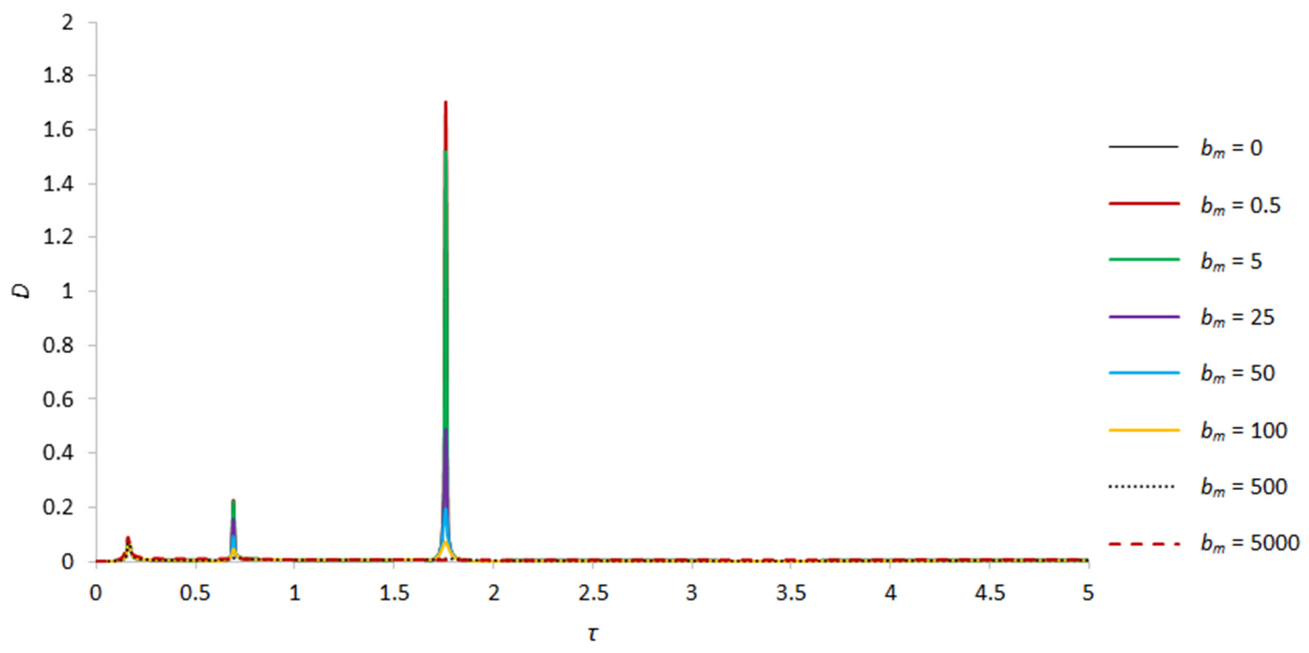
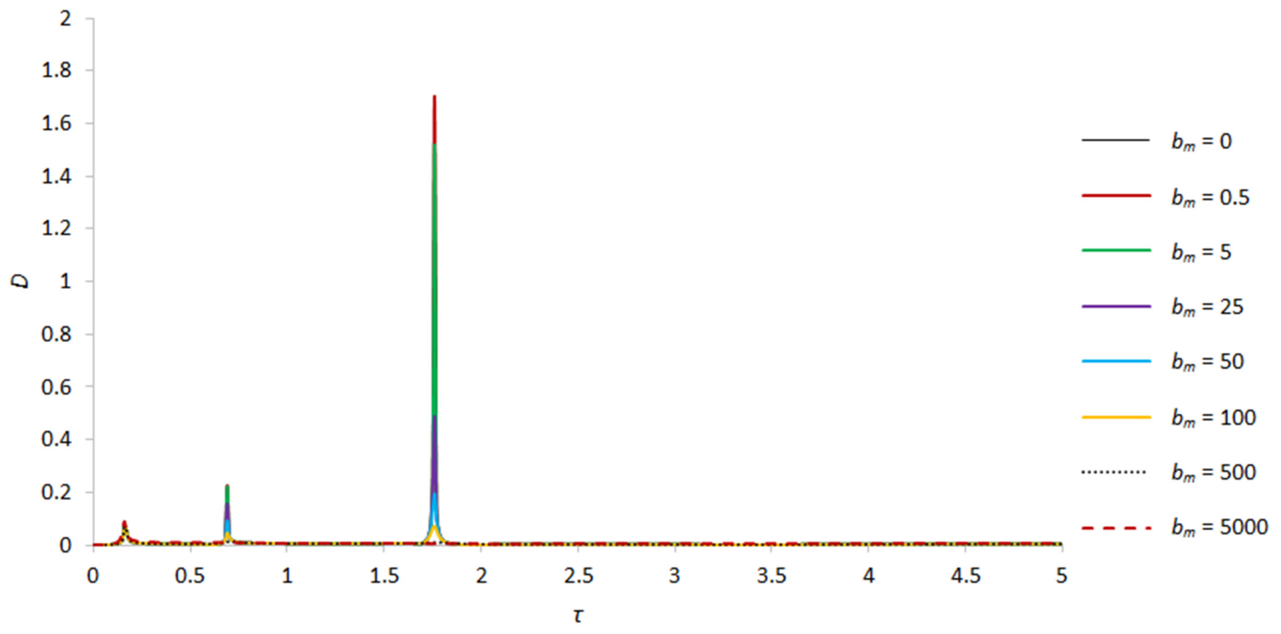
| D, γ = 4.56 | First Critical Speed Amplitude Value | Second Critical Speed Amplitude Value | Third Critical Speed Amplitude Value |
| bm = 0 | 0.07047227, τ = 0.16 | 0.226388549, τ = 0.69 | 1.704994351, τ = 1.76 |
| bm = 0.5 | 0.070468917, τ = 0.16 | 0.226287308, τ = 0.69 | 1.70381006, τ = 1.76 |
| bm = 5 | 0.07043893, τ = 0.16 | 0.221699183, τ = 0.69 | 1.520112352, τ = 1.76 |
| bm = 25 | 0.070309814, τ = 0.16 | 0.157597686, τ = 0.69 | 0.488944743, τ = 1.76 |
| bm = 50 | 0.070157935, τ = 0.16 | 0.034896767, τ = 0.7 | 0.194103909, τ = 1.76 |
| bm = 100 | 0.069885617, τ = 0.16 | 0.045941501, τ = 0.69 | 0.072065559, τ = 1.76 |
| bm = 500 | 0.069093807, τ = 0.16 | 0.012824952, τ = 0.7 | 0.010085603, τ = 1.77 |
| bm = 5000 | 0.089252733, τ = 0.16 | – | – |
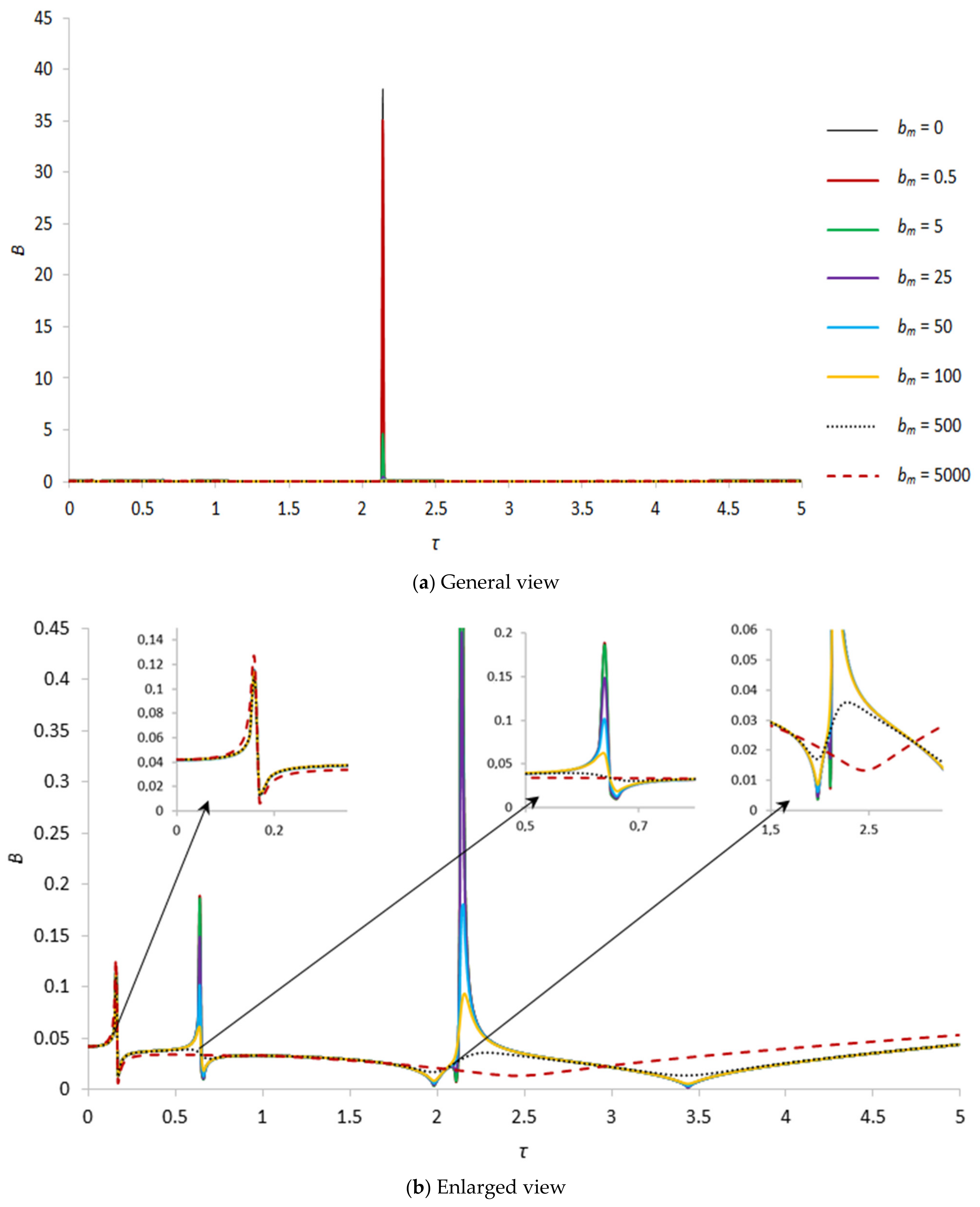
| B, γ = 2.6 | First Critical Speed Amplitude Value | Second Critical Speed Amplitude Value | Third Critical Speed Amplitude Value |
|---|---|---|---|
| bm = 0 | 0.188180917, τ = 0.64 | 38.0983794, τ = 2.14 | |
| bm = 0.5 | 0.188128512, τ = 0.64 | 35.05368501, τ = 2.14 | |
| bm = 5 | 0.114550189, τ = 0.16 | 0.185743424, τ = 0.64 | 4.620198303, τ = 2.14 |
| bm = 25 | 0.114543039, τ = 0.16 | 0.148131171, τ = 0.64 | 0.442357104, τ = 2.14 |
| bm = 50 | 0.113852547, τ = 0.16 | 0.100918717, τ = 0.64 | 0.180448011, τ = 2.15 |
| bm = 100 | 0.113189756, τ = 0.16 | 0.06088884, τ = 0.64 | 0.093096022, τ = 2.16 |
| bm = 500 | 0.109089699, τ = 0.16 | – | – |
| bm = 5000 | 0.124710542, τ = 0.16 | – | – |
| D, γ = 2.6 | First Critical Speed Amplitude Value | Second Critical Speed Amplitude Value | Third Critical Speed Amplitude Value |
| bm = 0 | 0.074299992, τ = 0.16 | 0.130906778, τ = 0.64 | 37.42981166, τ = 2.14 |
| bm = 0.5 | 0.074296638, τ = 0.16 | 0.130872119, τ = 0.64 | 34.43775859, τ = 2.14 |
| bm = 5 | 0.074266809, τ = 0.16 | 0.129169584, τ = 0.64 | 4.531230535, τ = 2.14 |
| bm = 25 | 0.074142119, τ = 0.16 | 0.101854993, τ = 0.64 | 0.417323892, τ = 2.14 |
| bm = 50 | 0.074004213, τ = 0.16 | 0.067028512, τ = 0.64 | 0.148186179, τ = 2.14 |
| bm = 100 | 0.073787317, τ = 0.16 | 0.036021818, τ = 0.64 | 0.053425977, τ = 2.14 |
| bm = 500 | 0.074595252, τ = 0.16 | 0.01092513, τ = 0.66 | 0.007393946, τ = 2.14 |
| bm = 5000 | 0.140446071, τ = 0.16 | – | – |

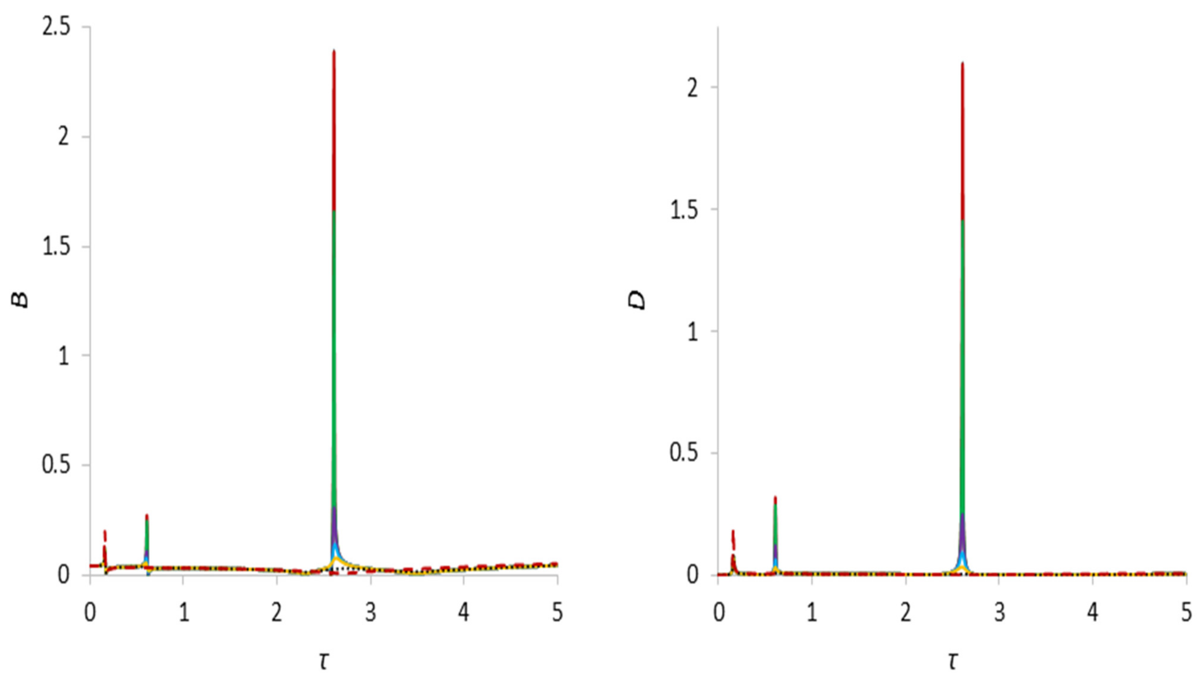
| B, γ = 1.67 | First Critical Speed Amplitude Value | Second Critical Speed Amplitude Value | Third Critical Speed Amplitude Value |
|---|---|---|---|
| bm = 0 | 0.118574461, τ = 0.16 | 0.27197385, τ = 0.61 | 2.395991343, τ = 2.61 |
| bm = 0.5 | 0.11856806, τ = 0.16 | 0.271326026, τ = 0.61 | 2.386092738, τ = 2.61 |
| bm = 5 | 0.118510785, τ = 0.16 | 0.244571454, τ = 0.61 | 1.657566825, τ = 2.61 |
| bm = 25 | 0.118263621, τ = 0.16 | 0.108761599, τ = 0.61 | 0.307975554, τ = 2.61 |
| bm = 50 | 0.117971542, τ = 0.16 | 0.079987206, τ = 0.61 | 0.141437807, τ = 2.61 |
| bm = 100 | 0.117443017, τ = 0.16 | 0.058212949, τ = 0.6 | 0.078056973, τ = 2.61 |
| bm = 500 | 0.115713077, τ = 0.16 | – | – |
| bm = 5000 | 0.200140464, τ = 0.16 | – | – |
| D, γ = 1.67 | First Critical Speed Amplitude Value | Second Critical Speed Amplitude Value | Third Critical Speed Amplitude Value |
| bm = 0 | 0.078416443, τ = 0.16 | 0.319661082, τ = 0.61 | 2.101480075, τ = 2.61 |
| bm = 0.5 | 0.078413261, τ = 0.16 | 0.318899815, τ = 0.61 | 2.092707266, τ = 2.61 |
| bm = 5 | 0.078385116, τ = 0.16 | 0.286969287, τ = 0.61 | 1.448573522, τ = 2.61 |
| bm = 25 | 0.078270549, τ = 0.16 | 0.122332756, τ = 0.61 | 0.248941102, τ = 2.61 |
| bm = 50 | 0.078151336, τ = 0.16 | 0.064906783, τ = 0.61 | 0.091711735, τ = 2.61 |
| bm = 100 | 0.077991713, τ = 0.16 | 0.03343016, τ = 0.6 | 0.034567932, τ = 2.61 |
| bm = 500 | 0.080131667, τ = 0.16 | – | – |
| bm = 5000 | 0.193818388, τ = 0.16 | – | – |
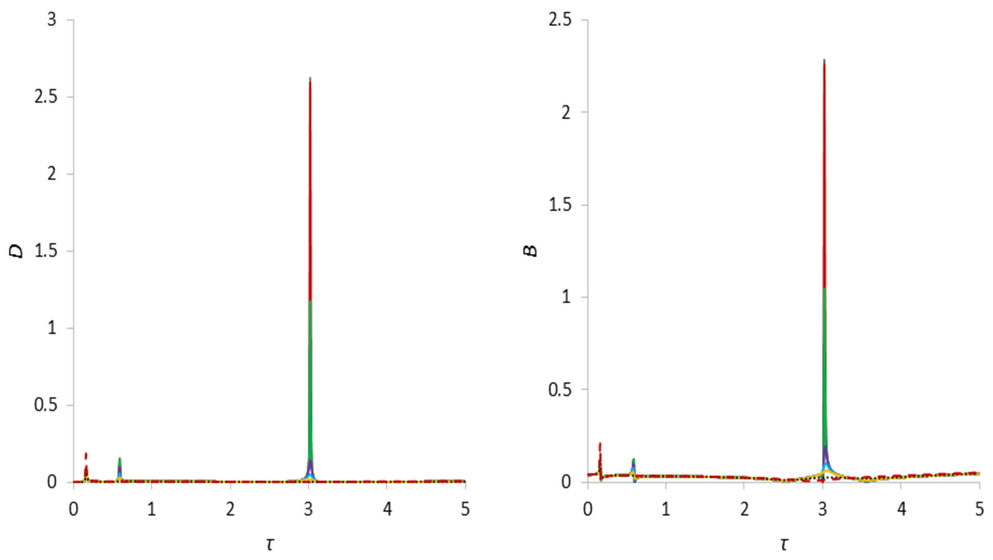
| B, γ = 1.25 | First Critical Speed Amplitude Value | Second Critical Speed Amplitude Value | Third Critical Speed Amplitude Value |
|---|---|---|---|
| bm = 0 | 0.121638282, τ = 0.16 | 0.122951082, τ = 0.59 | 2.281429046, τ = 3.02 |
| bm = 0.5 | 0.121632639, τ = 0.16 | 0.122901957, τ = 0.59 | 2.25145796, τ = 3.02 |
| bm = 5 | 0.121582276, τ = 0.16 | 0.121641647, τ = 0.59 | 1.035804071, τ = 3.02 |
| bm = 25 | 0.121367604, τ = 0.16 | 0.098499341, τ = 0.58 | 0.166361948, τ = 3.02 |
| bm = 50 | 0.121120227, τ = 0.16 | 0.078839058, τ = 0.58 | 0.103151902, τ = 3.02 |
| bm = 100 | 0.120694759, τ = 0.16 | 0.055532351, τ = 0.58 | 0.06308127, τ = 3.02 |
| bm = 500 | 0.120406103, τ = 0.16 | – | – |
| bm = 5000 | 0.210144507, τ = 0.16 | – | – |
| D, γ = 1.25 | First Critical Speed Amplitude Value | Second Critical Speed Amplitude Value | Third Critical Speed Amplitude Value |
| bm = 0 | 0.081552542, τ = 0.16 | 0.154403646, τ = 0.59 | 2.6271788, τ = 3.02 |
| bm = 0.5 | 0.081549629, τ = 0.16 | 0.154341266, τ = 0.59 | 2.59220114, τ = 3.02 |
| bm = 5 | 0.081523936, τ = 0.16 | 0.152395469, τ = 0.59 | 1.173065248, τ = 3.02 |
| bm = 25 | 0.081421162, τ = 0.16 | 0.098951316, τ = 0.58 | 0.14148849, τ = 3.02 |
| bm = 50 | 0.081318754, τ = 0.16 | 0.03067025, τ = 0.59 | 0.051515196, τ = 3.02 |
| bm = 100 | 0.081199692, τ = 0.16 | 0.055532351, τ = 0.59 | 0.020073614, τ = 3.02 |
| bm = 500 | 0.083967196, τ = 0.16 | – | – |
| bm = 5000 | 0.186578729, τ = 0.16 | – | – |
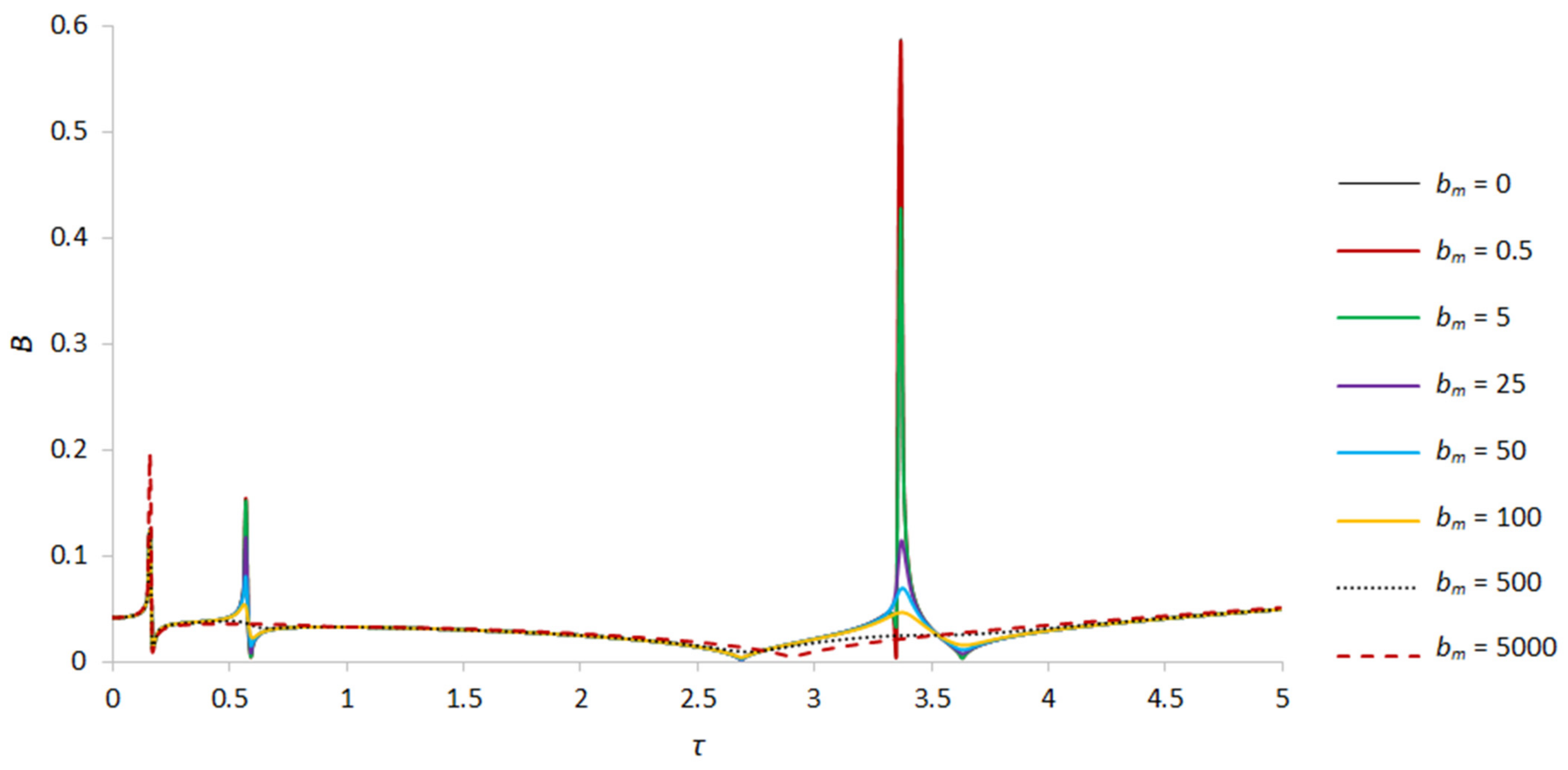
| B, γ = 1.03 | First Critical Speed Amplitude Value | Second Critical Speed Amplitude Value | Third Critical Speed Amplitude Value |
|---|---|---|---|
| bm = 0 | 0.123836133, τ = 0.16 | 0.154082698, τ = 0.57 | 0.582653298, τ = 3.37 |
| bm = 0.5 | 0.123831142, τ = 0.16 | 0.15403417, τ = 0.57 | 0.580389919, τ = 3.37 |
| bm = 5 | 0.123786664, τ = 0.16 | 0.151690752, τ = 0.57 | 0.425847453, τ = 3.37 |
| bm = 25 | 0.123598669, τ = 0.16 | 0.117230408, τ = 0.57 | 0.114353556, τ = 3.37 |
| bm = 50 | 0.123385864, τ = 0.16 | 0.080130589, τ = 0.57 | 0.069492128, τ = 3.38 |
| bm = 100 | 0.123033788, τ = 0.16 | 0.054080999, τ = 0.56 | 0.046679793, τ = 3.37 |
| bm = 500 | 0.123518243, τ = 0.16 | – | – |
| bm = 5000 | 0.196425395, τ = 0.16 | – | – |
| D, γ = 1.03 | First Critical Speed Amplitude Value | Second Critical Speed Amplitude Value | Third Critical Speed Amplitude Value |
| bm = 0 | 0.083803356, τ = 0.16 | 0.101565041, τ = 0.57 | 0.124078552, τ = 3.35 |
| bm = 0.5 | 0.083800714, τ = 0.16 | 0.101535013, τ = 0.57 | 0.123990942, τ = 3.35 |
| bm = 5 | 0.08377746, τ = 0.16 | 0.099920685, τ = 0.57 | 0.115971317, τ = 3.35 |
| bm = 25 | 0.083685484, τ = 0.16 | 0.075582465, τ = 0.57 | 0.050630183, τ = 3.35 |
| bm = 50 | 0.08359651, τ = 0.16 | 0.048524802, τ = 0.57 | 0.022746045, τ = 3.35 |
| bm = 100 | 0.083504258, τ = 0.16 | 0.028624914, τ = 0.58 | 0.010481636, τ = 3.33 |
| bm = 500 | 0.08647026, τ = 0.16 | 0.009075681, τ = 0.62 | – |
| bm = 5000 | 0.165670988, τ = 0.16 | – | – |

6. Conclusions
Author Contributions
Funding
Institutional Review Board Statement
Informed Consent Statement
Data Availability Statement
Acknowledgments
Conflicts of Interest
References
- Kydyrbekuly, A.; Zhauyt, A.; Ibrayev, G.-G.A. Investigation of Nonlinear Forced Vibrations of the “Rotor-Movable Foundation” System on Rolling Bearings by the Jacobi Elliptic Functions Method. Appl. Sci. 2022, 12, 7042. [Google Scholar] [CrossRef]
- Kydyrbekuly, A.; Ibrayev, G.G.A.; Ospan, T.; Nikonov, A. Multi-parametric Dynamic Analysis of a Rolling Bearings System. Strojniski Vestnik. J. Mech. Eng. 2021, 67, 421–432. [Google Scholar] [CrossRef]
- Feng, N.; Hahn, E. Experimental identification of the foundation in a rotor-bearing-foundation system. In Proceedings of the 5th IFToMM International Conference on Rotor Dynamics, Darmstadt, Germany, 7–10 September 1998; pp. 734–745. [Google Scholar]
- Saito, Y.; Sawada, T. Liquid sloshing in a rotating, laterally oscillating cylindrical container. Univers. J. Mech. Eng. 2017, 5, 97–101. [Google Scholar] [CrossRef]
- Eswaran, M.; Saha, U.K. Sloshing of Liquids in Partially Filled Tanks-A Review of Experimental Investigations. Ocean. Syst. Eng. 2011, 1, 131–155. [Google Scholar] [CrossRef]
- Tchomeni, B.X.; Alugongo, A. Modelling and numerical simulation of vibrations induced by mixed faults of a rotor system immersed in an incompressible viscous fluid. Adv. Mech. Eng. 2018, 10, 1–21. [Google Scholar] [CrossRef]
- Behera, R.K.; Parhi, D.R.; Sahu, S.K. Vibration analysis of a cracked rotor surrounded by viscous liquid. J. Vib. Control 2006, 12, 465–494. [Google Scholar] [CrossRef]
- Tarapov, I.E. On the basic equations and problems of the hydrodynamics of polarizable and magnetizable media. Theory Funct. Funct. Anal. Their Appl. 1973, 15, 221–239. [Google Scholar]
- Shimogo, T.; Kazao, Y. Critical speed of rotor in a liquid. Bull. JSME 1982, 25, 277–283. [Google Scholar] [CrossRef]
- Kydyrbekuly, A.; Khajiyeva, L.; Gulama-Garyp, A.Y. Nonlinear vibrations of a rotor-fluid-foundation system supported by rolling bearings. Stroj. Vestn./J. Mech. Eng. 2016, 62, 351–362. [Google Scholar] [CrossRef]
- Al-Bedoor, B.O. Transient torsional and lateral vibrations of unbalanced rotors with rotor-to-stator rubbing. J. Sound Vib. 2000, 229, 627–645. [Google Scholar] [CrossRef]
- Tchomeni, B.X.; Alugongo, A.A.; Masu, L.M. A fault analysis cracked-rotor-to-stator rub and unbalance by vibration analysis technique. Int. J. Mech. Aerospace Ind. Mechatr. Manuf. Eng. 2015, 9, 1883–1892. [Google Scholar]
- Stewartson, K. On the stability of a spinning top containing liquid. J. Fluid Mech. 1959, 5, 577–592. [Google Scholar] [CrossRef]
- Bauer, H.F.; Eidel, W. Axisymmetric oscillations in a slowly rotating cylindrical container filled with viscous liquid. Eng. Res. 1997, 63, 215–223. [Google Scholar]
- Kimura, K.; Takahara, H.; Sakata, M. Effects of higher order radial modes upon nonlinear sloshing in a circular cylindrical tank subjected to vertical excitation. Trans. JSMEC 1994, 60, 3259–3267. [Google Scholar] [CrossRef]
- Bauer, H.F. Natural frequencies and response of spinning liquid column with apparently sliding contact line. Acta Mech. 1993, 97, 115–122. [Google Scholar] [CrossRef]
- Awrejcewicz, J.; Dzyubak, L.P. 2-DOF non-linear dynamics of a rotor suspended in the magneto-hydrodynamic field in the case of soft and rigid magnetic materials. Int. J. Non-Linear Mech. 2010, 45, 919–930. [Google Scholar] [CrossRef]
- Awrejcewicz, J.; Dzyubak, L.P. Chaos caused by hysteresis and saturation phenomenon in 2-DOF vibrations of the rotor supported by the magneto-hydrodynamic bearing. Int. J. Bifurc. Chaos 2011, 21, 2801–2823. [Google Scholar] [CrossRef]
- Ji, J.C.; Hansen, C.H. Non-linear oscillations of a rotor in active magnetic bearings. J. Sound Vib. 2001, 240, 599–612. [Google Scholar] [CrossRef]
- Ji, J.C.; Leung, A. Non-linear oscillations of a rotor-magnetic bearing system under superharmonic resonance conditions. Int. J. Non-Linear Mech. 2003, 38, 829–835. [Google Scholar] [CrossRef]
- Kamel, M.; Bauomy, H. Nonlinear oscillation of a rotor-AMB system with time varying stiffness and multi-external excitations. J. Vib. Acoust. 2009, 131, 031009. [Google Scholar] [CrossRef]
- Saeed, N.A.; Kamel, M. Nonlinear PD-controller to suppress the nonlinear oscillations of horizontally supported Jeffcott-rotor system. Int. J. Non-Linear Mech. 2016, 87, 109–124. [Google Scholar] [CrossRef]
- Galdi, G.P.; Mazzone, G.; Zunino, P. Inertial Motions of a Rigid Body with a Cavity Filled with a Viscous Fluid. Comptes Rendus Mec. 2013, 341, 760–765. [Google Scholar] [CrossRef]
- Kuang, J.L.; Leung, A.Y.T.; Tan, S. Chaotic Attitude Oscillations of a Satellite Filled with a Rotating Ellipsoidal Mass of Liquid Subject to Gravity-Gradient Torgues. Chaos 2004, 14, 111–117. [Google Scholar] [CrossRef] [PubMed]
- Leung, A.Y.T.; Kuang, J.L. Chaotic Rotations of a Liquid- Filled Solid. J. Sound Vib. 2007, 302, 540–563. [Google Scholar] [CrossRef]
- Baozeng, Y.; Xie, J. Chaotic Attitude Maneuvers in Spacecraft with Completety Liquid—Filled Cavity. J. Sound Vib. 2007, 302, 643–656. [Google Scholar] [CrossRef]
- Ishiyama, T.; Kaneko, S.; Takemoto, S.; Sawada, T. Relation Between Dynamic Pressure and Displacement of Free Surface in Two-Layer Sloshing Between a Magnetic Fluid and Silicone Oil. Mater. Sci. Forum. 2014, 792, 33–38. [Google Scholar] [CrossRef]
- Romero-Calvo, Á.; Cano Gómez, G.; Castro-Hernández, E.; Maggi, F. Free and forced oscillations of magnetic liquids under low-gravity conditions. J. Appl. Mech. 2020, 87, 021010. [Google Scholar] [CrossRef]
- Saeed, N.A.; El-Ganaini, W. Time-delayed control to suppress the nonlinear vibrations of a horizontally suspended Jeffcott-rotor system. Appl. Math. Model. 2017, 44, 523–539. [Google Scholar] [CrossRef]
- Sekhar, A.S.; Prabhu, B.S. Condition monitoring of cracked rotors through transient response. Mech. Mach. Theory 1998, 33, 1167–1175. [Google Scholar] [CrossRef]
- Derendyayev, N.V.; Soldatov, I.N.; Vostrukhov, A.V. Stability and Andronov-Hopf bifurcation of steady-state motion of rotor system partly filled with liquid: Continuous and discrete models. J. Appl. Mech. 2006, 73, 580–589. [Google Scholar] [CrossRef]
- Manasseh, R. Distortions of inertia waves in a rotating fluid cylinder forced near its fundamental mode resonance. J. Fluid Mech. 1994, 265, 345–370. [Google Scholar] [CrossRef]
- Zhu, C. Experimental investigation into the effect of fluid viscosity on instability of an overhung flexible rotor partially filled with fluid. J. Vib. Acoust. 2006, 128, 392–401. [Google Scholar]
- Urbiola-Soto, L.; Lopez-Parra, M. Liquid self-balancing device effects on flexible rotor stability. Shock Vib. 2013, 20, 109–121. [Google Scholar] [CrossRef]
- Harsha, S.P. Non-linear dynamic response of a balanced rotor supported on rolling element bearings. Mech. Syst. Signal Process. 2005, 19, 551–578. [Google Scholar] [CrossRef]
- Tiwari, M.; Gupta, K.; Prakash, O. Effect of radial internal clearance of a ball bearing on the dynamics of a balanced horizontal rotor. J. Sound Vib. 2000, 238, 723–756. [Google Scholar] [CrossRef]
- Tiwari, M.; Gupta, K.; Prakash, O. Dynamic response of an unbalanced rotor supported on ball bearings. J. Sound Vib. 2000, 238, 757–779. [Google Scholar] [CrossRef]
- Harsha, S.P. Nonlinear dynamic analysis of a highspeed rotor supported by rolling element bearings. J. Sound Vib. 2006, 290, 65–100. [Google Scholar] [CrossRef]
- Bai, C.; Zhang, H.; Xu, Q. Experimental and numerical studies on nonlinear dynamic behavior of rotor system supported by ball bearings. J. Eng. Gas Turbine Power. 2010, 132, 082502. [Google Scholar] [CrossRef]
- Harsha, S.P.; Sandeep, K.; Prakash, R. The effect of speed of balanced rotor on nonlinear vibrations associated with ball bearings. Int. J. Mech. Sci. 2003, 47, 225–240. [Google Scholar] [CrossRef]
- Savin, L.; Solomin, O.; Ustinov, D. Rotor dynamics on friction bearings with cryogenic lubrication. In Proceedings of the 10th World Congress on the Theory of Machine and Mechanisms, Oulu, Finland, 20–24 June 1999; Volume 4, pp. 1716–1721. [Google Scholar]
- Silin, R.; Royzman, V. The research into the automatic balancing process of rotors with vertical axis of rotation. In Proceedings of the 10th World Congress on the Theory of Machine and Mechanisms, Oulu, Finland, 20–24 June 1999; Volume 4, pp. 1734–1739. [Google Scholar]
- Ji, J.C.; Hansen, C.H.; Zander, A.C. Nonlinear dynamics of magnetic bearing systems. J. Intell. Mater. Syst. Struct. 2008, 19, 1471–1491. [Google Scholar] [CrossRef]
- Saeed, N.A.; Eissa, M.; El-Ganini, W.A. Nonlinear oscillations of rotor active magnetic bearings system. Nonlinear Dyn. 2013, 74, 1–20. [Google Scholar] [CrossRef]
- Du, T.C.; Geng, H.; Wang, B.; Lin, H.; Yu, L. Nonlinear oscillation of active magnetic bearing–rotor systems with a time-delayed proportional–derivative controller. Nonlinear Dyn. 2022, 109, 2499–2523. [Google Scholar] [CrossRef]
- Ji, J.C.; Yu, L.; Leung, A. Bifurcation behavior of a rotor supported by active magnetic bearings. J. Sound Vib. 2000, 235, 133–151. [Google Scholar] [CrossRef]
- Zhang, W.; Zhan, X.P. Periodic and chaotic motions of a rotor-active magnetic bearing with quadratic and cubic terms and time-varying stiffness. Nonlinear Dyn. 2005, 41, 331–359. [Google Scholar] [CrossRef]
- Zhang, W.; Yao, M.H.; Zhan, X.P. Multi-pulse chaotic motions of a rotor-active magnetic bearing system with time-varying stiffness. Chaos Solitons Fractals 2006, 27, 175–186. [Google Scholar] [CrossRef]
- Fylladitakis, E.D.; Theodoridis, M.P.; Moronis, A.X. Review on the history, research and applications of electrohydrodynamics. IEEE Trans. Plasma Sci. 2014, 42, 358–375. [Google Scholar] [CrossRef]
- Zhang, W.; Zu, J.W.; Wang, F.X. Global bifurcations and chaos for a rotor-active magnetic bearing system with time-varying stiffness. Chaos Solitons Fractals 2008, 35, 586–608. [Google Scholar] [CrossRef]
- Eissa, M.; Saeed, N.A.; El-Ganini, W.A. Saturation-based active controller for vibration suppression of a four-degree-of-freedom rotor-AMB system. Nonlinear Dyn. 2014, 76, 743–764. [Google Scholar] [CrossRef]
Disclaimer/Publisher’s Note: The statements, opinions and data contained in all publications are solely those of the individual author(s) and contributor(s) and not of MDPI and/or the editor(s). MDPI and/or the editor(s) disclaim responsibility for any injury to people or property resulting from any ideas, methods, instructions or products referred to in the content. |
© 2023 by the authors. Licensee MDPI, Basel, Switzerland. This article is an open access article distributed under the terms and conditions of the Creative Commons Attribution (CC BY) license (https://creativecommons.org/licenses/by/4.0/).
Share and Cite
Kydyrbekuly, A.; Zhauyt, A.; Ibrayev, G.-G.A. Parametric Analysis of Nonlinear Oscillations of the “Rotor–Weakly Conductive Viscous Fluid–Foundation” System under the Action of a Magnetic Field. Appl. Sci. 2023, 13, 12089. https://doi.org/10.3390/app132112089
Kydyrbekuly A, Zhauyt A, Ibrayev G-GA. Parametric Analysis of Nonlinear Oscillations of the “Rotor–Weakly Conductive Viscous Fluid–Foundation” System under the Action of a Magnetic Field. Applied Sciences. 2023; 13(21):12089. https://doi.org/10.3390/app132112089
Chicago/Turabian StyleKydyrbekuly, Almatbek, Algazy Zhauyt, and Gulama-Garip Alisher Ibrayev. 2023. "Parametric Analysis of Nonlinear Oscillations of the “Rotor–Weakly Conductive Viscous Fluid–Foundation” System under the Action of a Magnetic Field" Applied Sciences 13, no. 21: 12089. https://doi.org/10.3390/app132112089