Article

Snow Load Shape Coefficients and Snow Prevention Method for Stepped Flat Roofs

1
School of Civil Engineering, Shijiazhuang Tiedao University, Shijiazhuang 051132, China
2
State Key Laboratory of Mechanical Behavior and System Safety of Traffic Engineering Structures, Shijiazhuang Tiedao University, Shijiazhuang 050043, China
3
Key Laboratory of Roads and Railway Engineering Safety Control, Ministry of Education, Shijiazhuang Tiedao University, Shijiazhuang 050043, China
4
Innovation Center for Wind Engineering and Wind Energy Technology of Hebei Province, Shijiazhuang 050043, China
*
Author to whom correspondence should be addressed.
Appl. Sci. 2023, 13(22), 12109; https://doi.org/10.3390/app132212109
Submission received: 25 September 2023 / Revised: 2 November 2023 / Accepted: 5 November 2023 / Published: 7 November 2023
(This article belongs to the Section Civil Engineering)

Abstract

:
Excessive snow load and nonuniform snow deposition are the main factors leading to building collapses. The snow load shape coefficient represents the dimensionless snow load, and its value is related to the unbalanced distribution of snow. The snow load shape coefficients for stepped flat roofs vary greatly in the codes of different regions, which always leads to underestimation of snow loads. We need a widely used standard for snow load shape coefficients. Therefore, through a combination of field measurements and numerical simulations, this study probes the snow accumulation processes and snow load shape coefficients on stepped flat roofs and proposes an equation to calculate snow load shape coefficients and the optimal slope of snow protection for lower roofs. It is found that the maximum snow load shape coefficient emerges at the roof junction with a value of 3.44. The nonuniform length of the snow accumulation is equal to two times the level difference. Based on these, the equation of the snow load shape coefficients is summarized, which is combined with the discrepancies between different codes and the regularity of snow distributions. In this study, the dynamic grid technology under the Eulerian framework is used to successfully predict snow accumulation on stepped flat roofs, and it is noted that snow erosion and deposition are closely related to the location and size of vortexes. Finally, we consider that the ideal slope for the lower roof to prevent snow should be 11°.

1. Introduction

In recent years, extreme snow and ice disasters have occurred frequently around the world, resulting in a significant increase in building damage and collapse [1,2,3]. For example, in 2008, a major snowstorm in southern China caused the collapse of 485,000 buildings in total and a direct economic loss of USD 21 billion. In 2014, a sudden snowfall at the end of winter in China’s Xinjiang province toppled more than 200 houses and damaged 2600 others. Through a large number of post-disaster investigations, it was found that the main reasons for such accidents were excessive snow load and nonuniform snow deposition on the roof [4,5,6]. Unfortunately, there are discrepancies and distinctions between the snow load sections in the codes of different countries. Therefore, it is essential to clarify the distinctions between different national load codes and to conduct intensive research on the snowdrift characteristics on roofs.
The stepped flat roof is a typical snow-sensitive structure. In the current load codes/standards of countries (hereinafter called codes), the snow load values of stepped flat roofs are mainly measured via the field measurements of full-size roofs [7,8,9,10,11]. Since 1956, the Division of Building Research of the National Research Council of Canada has carried out field measurements of snow loads on multiple structures with actual stepped flat roofs, whose results have become the main basis for the modification of snow load codes [11]. By establishing a snowdrift database to statistically explore stepped flat roofs, the USA revised the section on the snow load shape coefficient of stepped flat roofs [10].
The field measurement of the full-size roof is the most intuitive and accurate. However, due to the actual roof’s large span and high snow storage, the final snow pattern is hard to obtain. As a result, reduced-scale field research has gradually developed [12,13,14,15]. Compared with prototype measurement, scaled measurement requires less time and provides more valuable information. Nevertheless, the size effect of snow particles is not yet clear. Fortunately, investigations have shown that equilibrium drifts of models at a scale ratio greater than 1:30 are approximately proportional to the ones of prototype models [13,14,16], and provide suggestions for the snow load shape coefficients of stepped flat roofs [12,16].
Due to the impact of the wind, a lower roof has a more easily unbalanced snow load, resulting in structurally weak areas. Therefore, different approaches are used to reduce the snow load on stepped flat roofs, such as manual operations for snow removal, roof heating systems, and improved roof structures. Manual operations for snow removal are only applicable to the roofs that one can set foot on. In addition, the cost of setting up roof heating systems is high, making them unsuitable for large-scale expansion. In contrast, improving the roof structure is relatively practical. The Guide to the Snow Load Provisions of ASCE 7-16 provides two suggestions for enhancing the structure of stepped flat roofs [17], as shown in Figure 1. The principle of both methods is to add components on the roof to reduce the space available for snowpack. Thus, it is necessary to clarify the snow accumulation processes and the final snow distribution on stepped flat roofs, to provide references and suggestions for the improvement of roof structures.
In conclusion, the snow load codes in different regions are difficult to reconcile, and there is no uniform standard for the stepped flat roof. These codes often obtain different snow load shape coefficients for the same case. Therefore, a harmonized equation to calculate the snow load shape coefficients of stepped flat roofs needs to be proposed. In addition, while raising the slope is well recognized in the scientific field, the optimal slope for the lower roof has still not been specified.
To investigate snow load shape coefficients and the optimal slope for stepped flat roofs, a series of field measurements and numerical simulations were carried out. First, scaled field observations were used to determine the snow pattern on stepped flat roofs. Based on the determination of the snow pattern, the snow load shape coefficients of stepped flat roofs under the final snow status were calculated. The polynomial of the snow load shape coefficients on stepped flat roofs was introduced, which applies to the snow load codes in different countries. Then, dynamic mesh technology modeled with the Eulerian–Eulerian method was successfully used to simulate the snow accumulation processes on stepped flat roofs. Finally, the optimal slope of the lower roof was clarified by comparison to prevent snow accumulation.

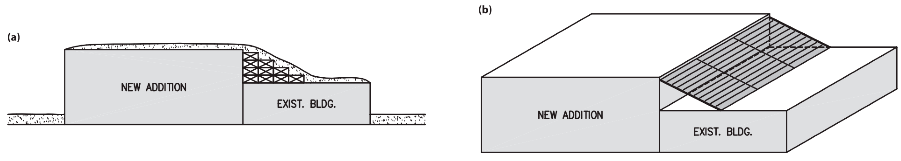
2. Field Measurement

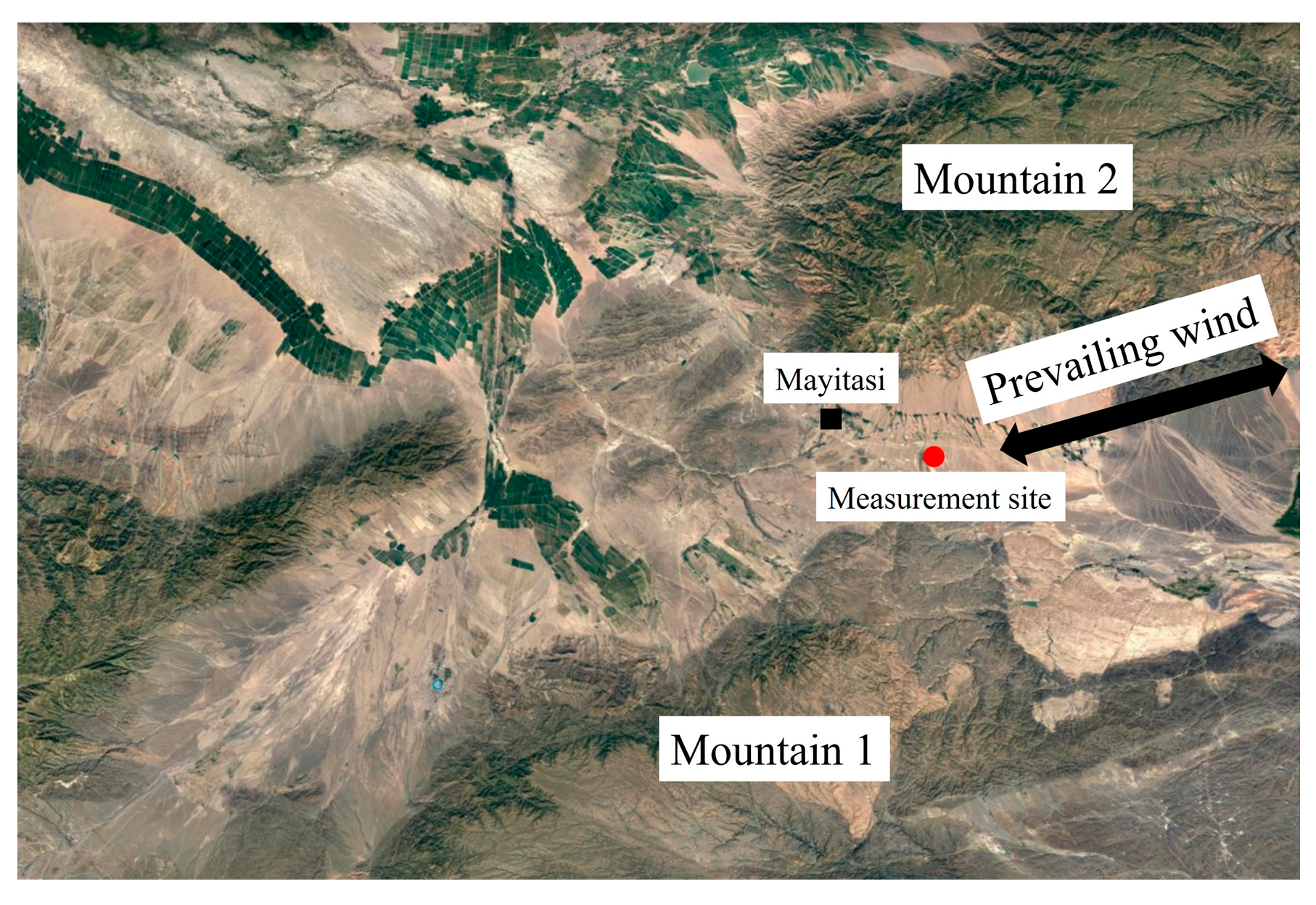
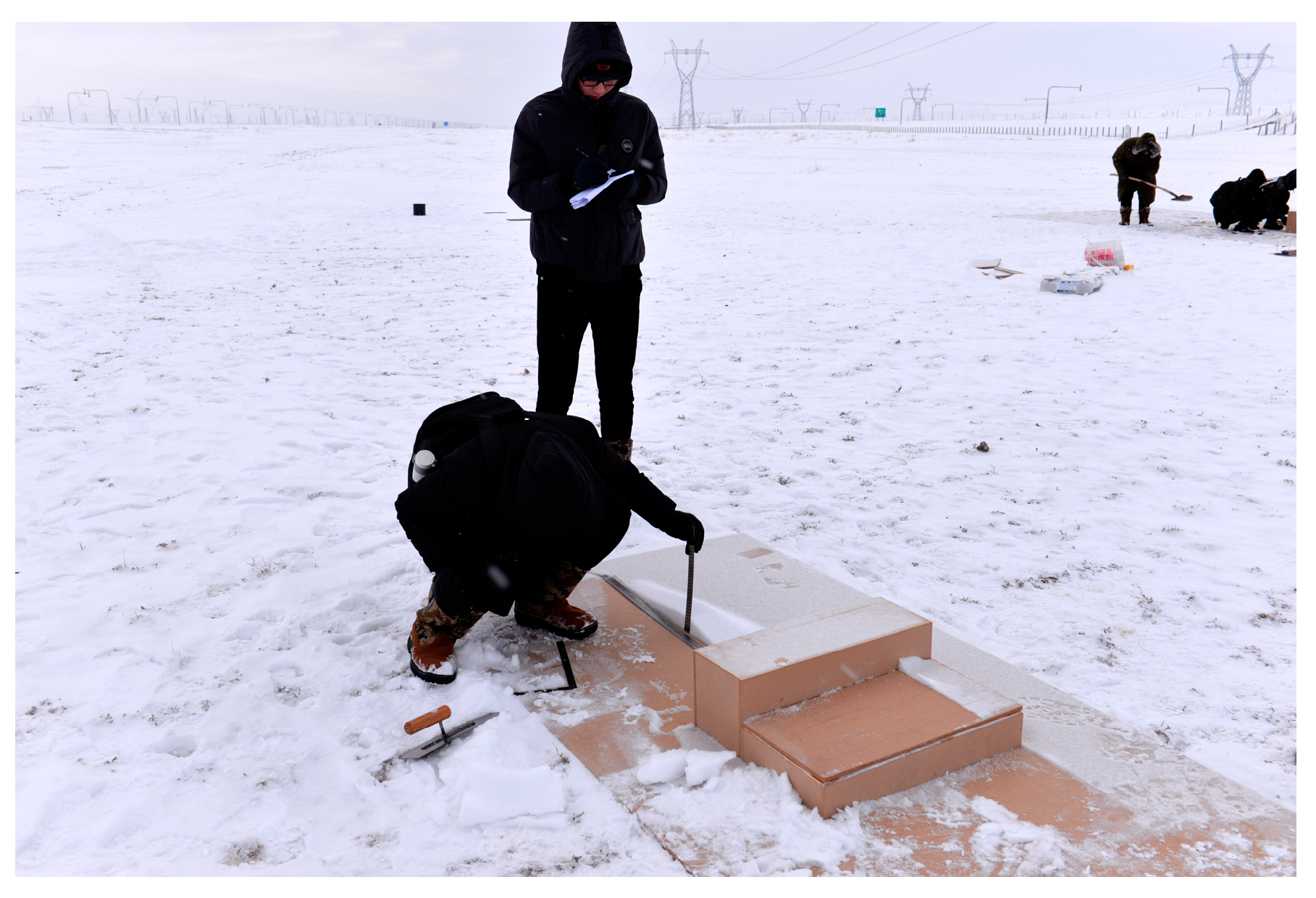
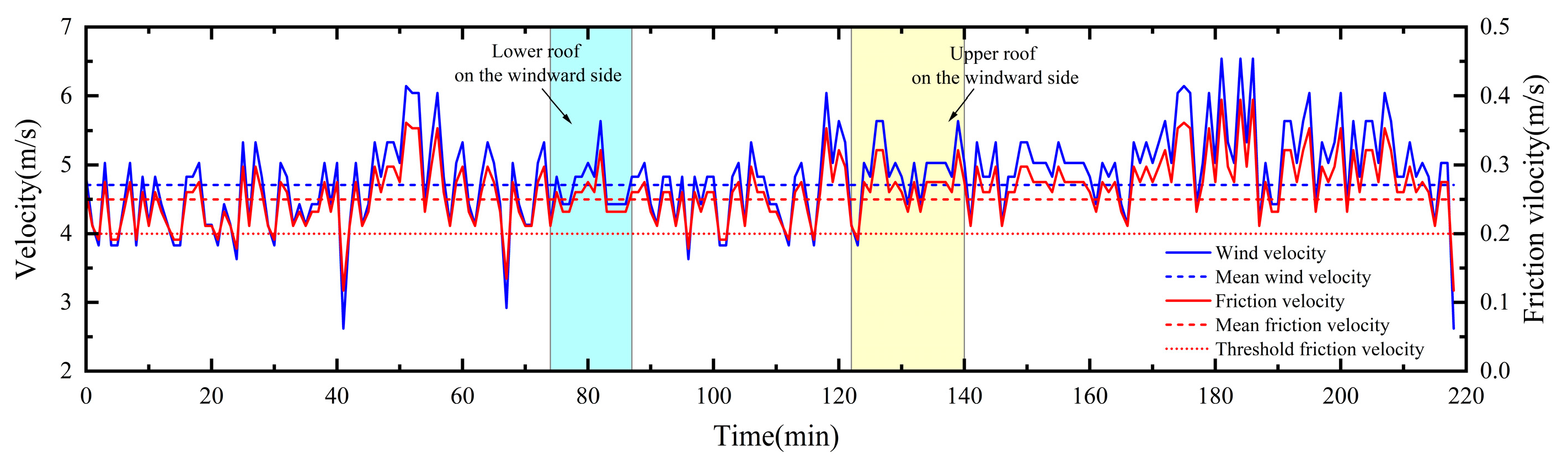
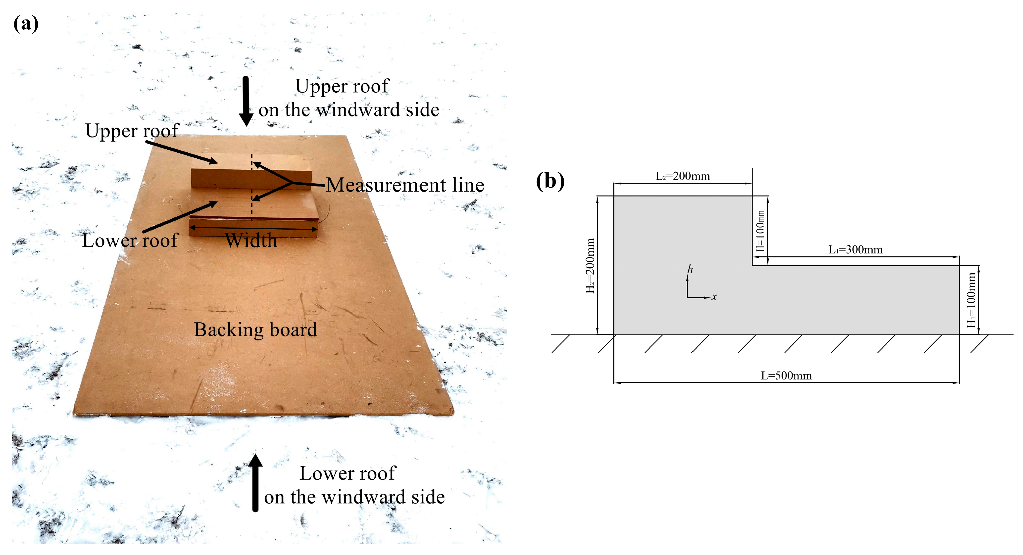
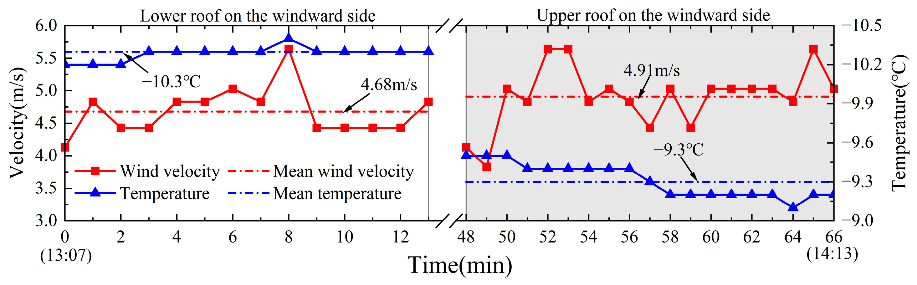
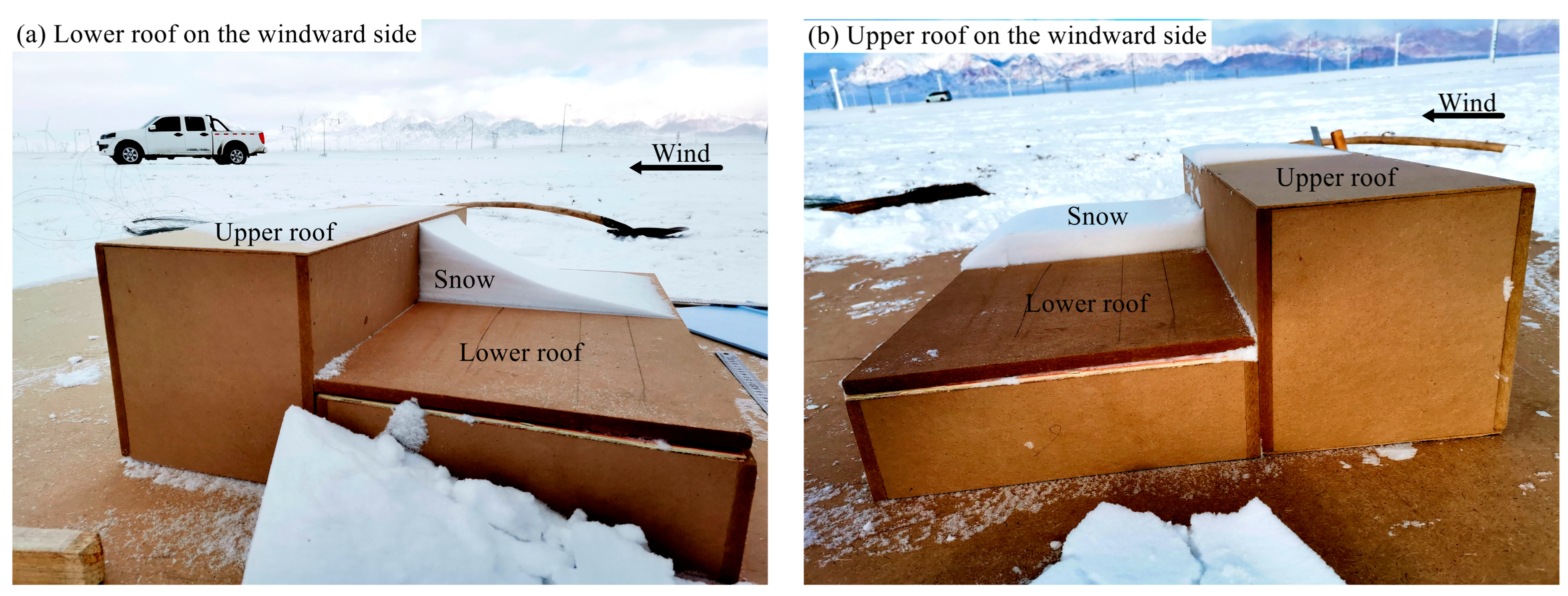
2.1. Field Site and Conditions

The field measurement site was in the Mayitas region of Xinjiang, which is located between two mountains 1500 m to 2000 m high. With the prevailing easterly winds, as shown in Figure 2, the maximum instantaneous wind speed could reach 40 m/s due to the “Venturi effect”. In 2018, the annual amount of snowfall in Mayitas was 122.6 mm, which was converted into about 1530 mm of snow depth. All field measurements were conducted at one site to avoid the influence of geographic factors, as shown in Figure 3.
The measurements were carried out on 25 December 2019. The YGY-QXY portable weather station was used to record the daily temperature, humidity, and instantaneous wind speed at a height of 1 m, with a time interval of 1 min. The average relative humidity was 69.2%. The average temperature was −9.6 °C, and the average wind speed was 4.82 m/s. The time history of the wind speed is shown in Figure 4. It is considered that the wind speed conforms to the logarithmic rate:
U ( z ) = u * κ ln z z 0 ,
where u* is the friction velocity, κ is the Karman constant equal to 0.42, and z is the vertical height above the ground.
The snow surface roughness length z0 is calculated using the empirical equation proposed by Pomeroy and Gray (1990) [18], referring to the field measurements:
z 0 = 0.12 u * 2 2 g .
The friction velocity (Figure 4) is obtained using Equations (1) and (2), and the threshold friction velocity is 0.2 m/s. The atmospheric friction velocity is 0.26 m/s, and the roughness length of the snow surface is 0.4 mm. The measurement lasted for 218 min. Artificial snowfall and natural blowing snow were combined to generate the final pattern of snow distribution on stepped flat roofs.

2.2. Model Parameter

Because of the limitations of the test site and conditions, a model of a stepped flat roof was made of plywood with a scale ratio of 1:25, as shown in Figure 5a. Figure 5b shows the model outline. The dimensions were as follows: 100 mm high (H2), 300 mm long (L1), and 600 mm wide at the lower roof and 100 mm high (H2), 200 mm long (L2), and 600 mm deep at the upper roof. The length ratio of the lower roof and the upper roof was 3:2, and the height ratio was 1:2.
In order to facilitate the measurement and leveling, a backing board was added to the bottom of the model. In the process of measurement, the status of the snowpack on the roof was maintained. When the snow reached the final distribution, a steel ruler and a drawing square were used to estimate the snow on the center line of the roof. The interval of the measured points was 2 cm. After one measurement, all the snow was removed from the roof and the board.

3. Numerical Simulation

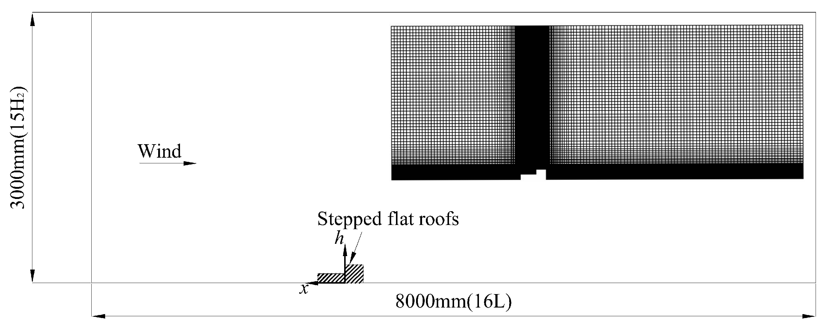
3.1. Simulation Scheme

In this study, the Euler–Euler method was adopted in which both the air phase and snow phase are regarded as a continuum. The proportions of the two phases in the mixture multiphase model are defined by the volume fraction. The continuity equation and momentum equation of the mixed phase are solved by the mixture model.
The continuity equation of the mixed phase is Equation (3):
t ρ m + ρ m v m = 0 .
The mixed phase density ( ρ m ) and the average mass velocity ( v m ) are determined using Equations (4) and (5):
ρ m = k = 1 2 α k ρ k ,
v m = k = 1 2 α k ρ k v k ρ m ,
where k = 1, 2 represents the principal term (air phase) and secondary term (snow phase), α k is the volume fraction of the kth term, ρ k is the density of the kth term, and v k is the velocity of the kth term.
The momentum equation for the mixture model is expressed as Equation (6):
t ρ m v m + ρ m v m v m = p + μ m v m + v m T + ρ m g + F k = 1 2 α k ρ k v d r , k v d r , k ,
where F is the volume force, and the mixed viscosity and the drift velocity of the kth term are calculated using Equations (7) and (8):
μ m = k = 1 2 α k μ k ,
v d r , k = v k v m .
The air phase is solved using the Reynolds equation [19]. The turbulence model adopts the realizable k-ε model [20,21], which improves the dissipation rate transport equation compared with the standard k-ε model. Zhao et al. (2016) [22] successfully simulated the wind field and snow distribution on stepped flat roofs with the help of the realizable k-ε model but did not consider the reverse impact of the snowpack on the wind field.
The management of the snow transport and movement in the computational domain is achieved using the snow phase volume fraction (Equation (9)) as well as the erosion and deposition models (Equations (10) and (11)) [23,24,25]. The governing equations are as follows:
t α 2 ρ 2 + α 2 ρ 2 v m = α 2 ρ 2 v dr , 2 ,
q e r o = A e r o u * 2 u * t 2 u * u * t ,
q d e p   = ϕ w f u * t 2 u * 2 u * t 2 u * < u * t ,
where Aero is the erosion constant, equal to 7.0 × 10⁻⁴ [23]; u* is the wall friction velocity; u*t is the threshold friction velocity of snow drifting; and Φ is the snow mass concentration.

3.2. Computational Parameters

Table 1 presents the major parameters in the field measurements and the numerical simulation. Ma et al. (2021b) [26] found that the probability distribution of the equivalent diameter of blowing snow particles meets the gamma distribution Ga(α, β), where α and β are the shape parameter and scale parameter (α = 2.94, β = 100.35), respectively, and the expected integrated snow particle size is 165 μm [27]. The measured snow density ranges from 120 kg/m3 to 300 kg/m3, and the snow density was 150 kg/m3 in the numerical simulation [28,29,30]. During snow transport, the diameter and the falling velocity of snow particles tend to be smaller in the higher part above the snow surface. Therefore, a lower falling speed (wf = 0.2 m/s) [28,30,31,32] was adopted in the higher part (h > 0.1 m), while in the lower part (h ≤ 0.1 m), a higher falling speed (wf = 0.35 m/s) was used [33,34]. The threshold friction velocity in the numerical simulation was 0.2 m/s [28,30], as illustrated in Figure 4.

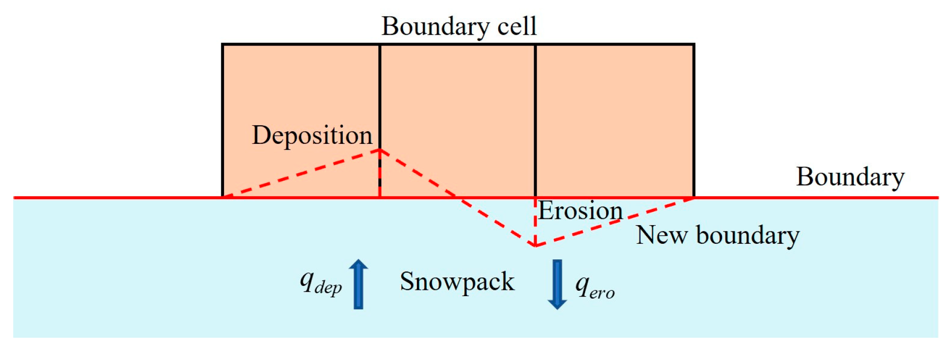
3.3. Calculation Settings

The study was carried out using ANSYS. In this work, a 2D model was adopted for simulation. The size of the numerical simulation model was the same as that of the model used in the field measurements, and the dimensions of the computational domain were 8000 mm (16 L) × 3000 mm (15 H2), as shown in Figure 6. The length of the rear flow field was 5000 mm (10 L) to fully develop the snow flow. In the processes of snow drift, the snow concentration above 1 m from the snow surface was almost 0; so, the height of the calculation domain was considered to be 3000 mm (15 H2).
The number of core grids accounts for more than 50% of the total grid. In order to maximize the quality of the grid around the model, an even grid with a height of 5 mm was adopted around the model. The mesh growth factor was 1.1 in the region far from the model, and the y+ value was controlled at about 80. The total number of meshes was about 30,000, the quality and orthogonality of the meshes were about 1, and the maximum aspect ratio of the meshes was less than 13.
The measured logarithmic wind speed profile was imposed by Equation (1) at the inlet, and the turbulent kinetic energy and dissipation rate were obtained using Equations (12) and (13) [35], with Cμ, the empirical constant, equal to 0.09.
k z = u A B L * 2 C μ
ε z = u A B L * 3 κ z
The inlet snow phase was defined by the volume fraction, which refers to Equations (14) and (15) derived by Kang et al. (2018) [34]:
f s a l   = ρ 3.29 ρ s u * 1 u * t 2 u * 2 ,
f s u s p   = f s a l   z h s a l   w f / κ u * ,
where hsal is the height of the saltation layer, which can be calculated using Equation (16) [18]:
h s a l = 1.6 u * 2 2 g .
The boundary of the ground and the model are set as the no-slip wall boundary, and the snow surface contour is updated in real time by using dynamic grid technology based on the transient method. The dynamic grid technology can consider the effect of the snow boundary on the airflow near the model and the trajectory of subsequent snow particles, to further improve the simulation accuracy [33,34]. The principle of the dynamic grid is shown in Figure 7.
For the values of the wall roughness height (KS) and roughness constant (CS), this work set the roughness constant CS = 2.0 [34]. Based on Equation (17) proposed by Blocken et al. (2007) [36], the roughness height of the wall was obtained as KS = 2 mm, which satisfies KS < yp, and yp is the center height of the minimum grid near the ground (yp = 2.5 mm).
K S = 9.793 z 0 C S
The upper boundary of the domain adopts a symmetry boundary, and the outlet is set as the pressure outlet. The calculation settings are summarized in Table 2.
To increase the credibility of our work, the methodological flow diagram is shown in Figure 8.

4. Results and Discussion

4.1. The Final Pattern of Snow Accumulation

The corresponding wind speed and temperature in the field measurements are illustrated in Figure 9. When the lower roof was on the windward side, the mean wind speed was 4.68 m/s, and the mean temperature was −10.3 °C. It took about 13 min to reach the final pattern of snow distribution. On the other hand, the windward snowdrift reached its final pattern in about 18 min, during which the mean wind speed was 4.91 m/s, and the mean temperature was −9.3 °C. The field measurements were conducted from 13:07 to 14:13, and the wind speed and temperature were relatively stable.
Figure 10 presents the measured snow deposition on the roof. In Figure 11, the horizontal axis denotes the distance from the upper wall x normalized by the level difference H, and the vertical axis denotes the dimensionless height h/H. The origin of the horizontal axis is located at the junction of the upper roof and the lower roof.
As indicated in Figure 10a and Figure 11a, when the lower roof was on the windward side, there was almost no snow accumulation on the upper roof. The final snow deposition on the lower roof was similar to a triangle, with the peak snow depth located at the roof junction (x/H = 0) and aligned with the outer edge of the upper roof (h/H = 2.0). The snow accumulation leveled off at x/H = 1.4. Due to the wind separation and acceleration occurring at x/H = 3, the lower roof presented a snow-free condition at x/H = 2.95~3.
Figure 10b and Figure 11b show the snow distribution when the upper roof was on the windward side. There was a small amount of snow on the upper roof. The peak snow depth was about 1/2H at x/H = 0. Similar to the appearance in Figure 10a and Figure 11a, the wind accelerated at the windward corner of the lower roof (x/H = −2), and the snow-free area occurred at x/H = −2~−1.8. The snow distribution on the lower roof was approximately uniform, and the dimensionless snow depth was around 0.4 at x/H = 0.2~2.4.

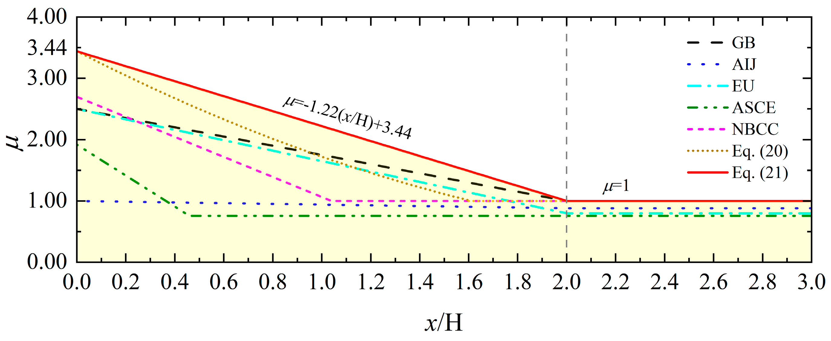
4.2. Snow Load Shape Coefficients

The snow depth d on the roof is normalized by the variation in snow depth Δd on the ground during the measurement. The dimensionless values obtained are regarded as snow load shape coefficients (μ), as shown in Figure 12.
The windward snow load shape coefficients on the lower roof gradually decreased with the increase in x/H. The snow load on the roof at x/H = 1.6 was the same as the ground snow load. The maximum snow load shape coefficient occurred at x/H = 0, μmax = 3.44. As indicated in Figure 12a, the snow load shape coefficients demonstrated a strong regularity, which was fitted with a quadratic polynomial of x/H to obtain Equation (18) (R2 = 0.9991):
μ = 0.3346 x / H 2 2.0547 x / H + 3.4426 .
The snow load shape coefficient of the lower roof when the upper roof was on the windward side (Figure 12b) was about 1 at x/H = 0.2~2.4. The snow load shape coefficient gradually decreased to 0.25 at x/H ≥ 2.4. However, this area was relatively small compared with the overall low roof; so, the snow load shape coefficient was still unified as 1. The maximum value of the shape coefficient on the lower roof occurred at the junction of the roofs (x/H = 0), μmax = 1.25. The snow load shape coefficient on the upper roof was smaller than that on the lower roof, and the maximum value was about 0.5.
The snow load on stepped flat roofs is specified in detail in many countries. However, the definitions of the snow load shape coefficient are different. Comparing the codes of different countries, the formula of the snow load values of roofs can be expressed in Equation (19) (the ASCE can also be derived to obtain this form), in which S is the snow load on the roof, μ is the snow load shape coefficient, and S0 is the ground snow load.
S = μ S 0
In this paper, the different expressions of snow load in different national load codes are unified into Equation (19). As listed in Table 3, the set of dimensionless coefficients that are multiplied by the S0 in each code is defined as the snow load shape coefficient. For easier comparison, the parameters with the same meanings in the formulas of different countries have been standardized.
The greater values of snow load shape coefficients at the same dimensionless distance are selected in two measurements, which are used to obtain the expressions for the snow load shape coefficients in this work as Equation (20):
μ = 0.3346 x / H 2 2.0547 x / H + 3.4426 0 x / H 1.6 1 x / H > 1.6 .
The fitting equation is compared with the snow load shape coefficients in different codes in Figure 13. Each code has fewer definitions of snow distribution on the upper roof, and the measured snow depth of the lower roof is much greater than that of the upper roof. Moreover, the snow load shape coefficients on the upper roof are far less than 1. Therefore, only the snow load shape coefficients for the lower roof are compared.
For stepped flat roofs, different national load codes hold that the maximum snow load shape coefficient emerges at the roof junction (x = 0), which is consistent with the measured results in this paper. However, the codes of different countries assume that the nonuniform distribution of snow load is a linear regularity. The measurement results justify that the law of quadratic polynomials is more suitable for expressing the snow distribution coefficients. Additionally, the maximum snow load shape coefficient in this paper is higher than that of other codes. The snow load shape coefficients of the AIJ code are the lowest in the snow load codes, with a maximum of only about 1. The ASCE code states that the unbalanced length of the snowpack only accounts for 1/6 of the roof span with snow load shape coefficients of less than 2. The snow load shape coefficients in NBCC are the highest among the other codes, whose maximum value is 2.7, but the nonuniform length of the snow accumulation is equal to the level difference (H). The EN and GB codes all consider that the length for the nonuniform area is 2/3 (2H) of the roof span, and the maximum snow load shape coefficient in the two codes is 2.5. The maximum snow load shape coefficients and the unbalanced length of snow are summarized in Table 4.
It is evident that the values of the snow load shape coefficients in different codes vary significantly due to the differences in the environmental and geographical characteristics of each country. This poses challenges in identifying the snow load of stepped flat roofs in practical projects. Therefore, the maximum snow load shape coefficients at each position and the maximum nonuniform length of deposition are summarized in Equation (21), which refers to the codes of different countries, and Equation (20).
μ = 1.22 x / H + 3.44 0 x / H 2 1 x / H > 2
Equation (20) states that the unbalanced length of the snow load on the lower roof is twice the level difference. The values of the snow load shape coefficient conform to linear regularity, with the maximum located at x = 0, and the maximum is about 3.44.

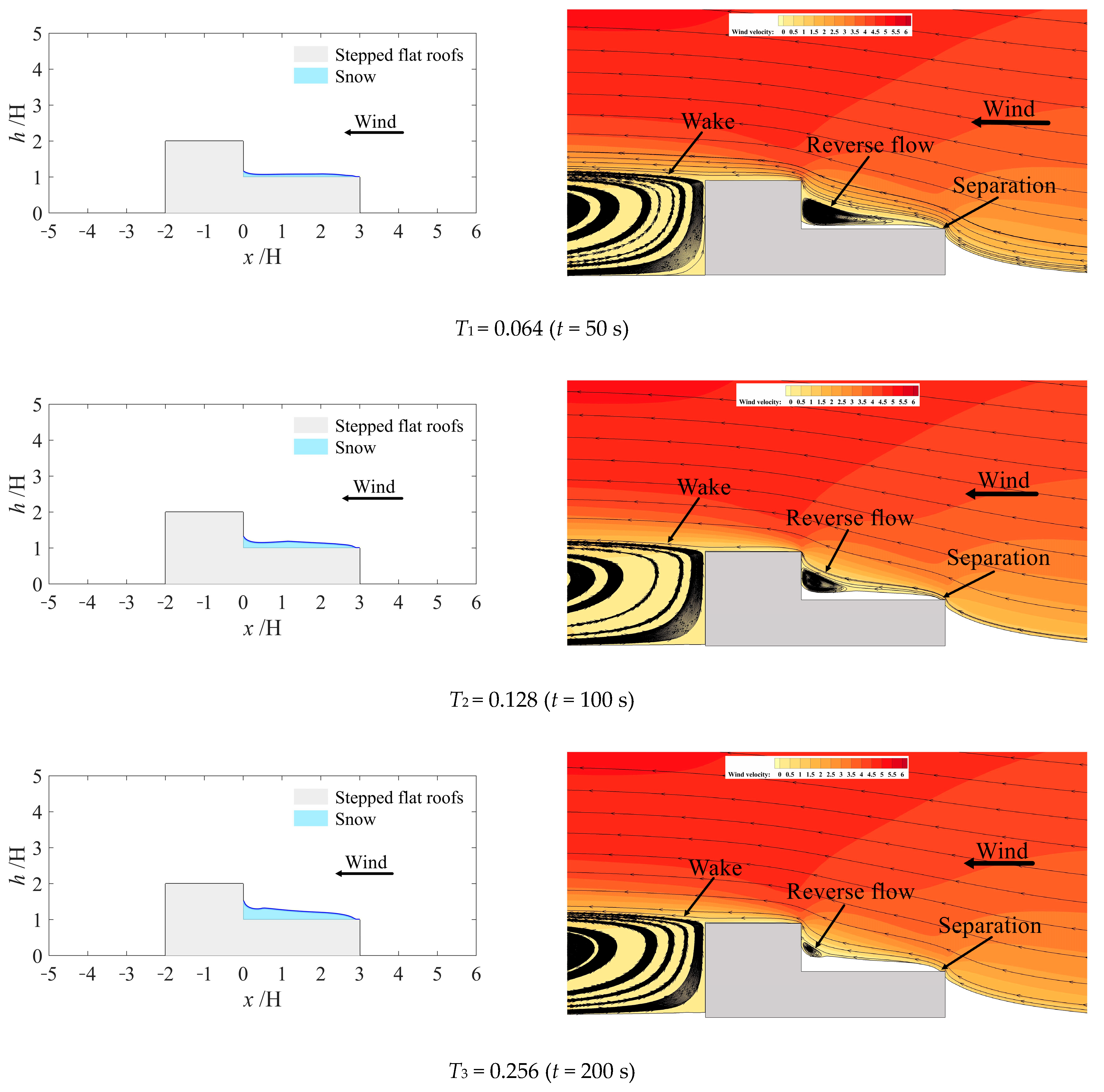
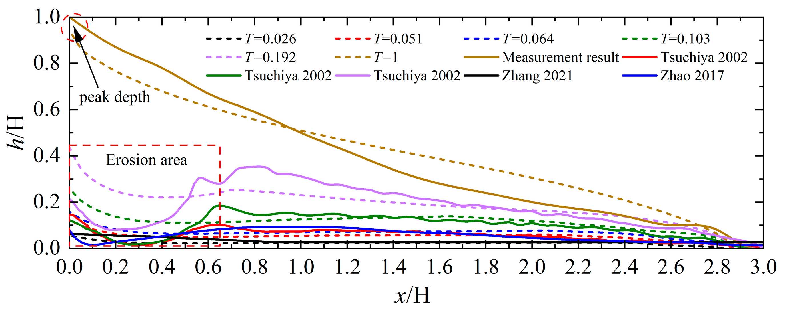
4.3. Snow Accumulation Processes for Stepped Flat Roofs

Based on the correspondences between the measurement results and codes, differences can be noted in the snow load shape coefficient values on stepped flat roofs. To explore the reasons, Figure 14 compares the snow accumulation processes on the stepped flat roof and flow fields around the roof at different times. The simulation time is 780 s, which is the same as the field-measured time. The dimensionless length of the erosion zone is defined as Le, and the time t of the snow accumulation is nondimensionalized to T = t/780. Correspondingly, T = 1 represents the time when the snow evolved into its final form. The snow shape on the lower roof was almost rectangular at T1 = 0.064, and the erosion and the deposition of snow were not obvious at this time. However, via the flow field analysis, it can be observed that a vortex with a dimensionless length of about 2 was formed on the lower roof, from which it can be inferred that this area was the erosion region. When the snow developed to T2 = 0.128, obvious erosion was observed due to the vortex on the lower roof. The dimensionless range of the erosion length was about 0~1. Over time, the erosion region gradually shrank. The vortex scale and the erosion length decreased to 0.5 at T3 = 0.256. The reverse flow on the lower roof disappeared at T4 = 0.385 when erosion was also not observed. It was concluded that erosion could be observed at T2 = 2T1, and the erosion length was reduced by half at T3 = 4T1. This indicates a linear relationship between the erosion length Le and the time T of the snow accumulation on stepped flat roofs; that is, Le = CT, where C is the proportional coefficient. The snow accumulation reached the final pattern at T5 = 1. In the processes of snow accumulation, a flow separation preventing deposition occurred at the end of the lower roof, which verifies the results observed in the measurement.
The simulation results of snow development are compared with the measurement results [12,14,22], as shown in Figure 15. The dotted lines indicate the numerical simulation results at different dimensionless times, while the solid lines represent the measurement results. The relative results are marked with the same color.
Figure 15 indicates that the simulation results are consistent with the field measurement results, and the erosion area and the peak depth of snow are reflected in the simulation results. Further comparison illustrates that different snow distributions in the literature correspond to different moments of snow accumulation on stepped flat roofs. Moreover, the corresponding times are all less than one-third of the snow accumulation time. This also proves that it is difficult for the snow on prototype structures to reach a stable state due to the influence of the measurement time and the environment.

4.4. Snow Prevention Method for Stepped Flat Roofs

According to the results of the measurements and numerical simulation, the final shape of the windward snow accumulation on the lower roof is approximated as a triangle. It can be predicted that increasing the angle of the lower roof can reduce the snow depth. Therefore, when the angle of the lower roof β is 1°~14°, the final snow distribution of the lower roof is obtained as shown in Figure 16. As the angle of the lower roof increases, the snow profile on the lower roof is virtually unchanged, but the amount of snow accumulation significantly decreases. To quantitatively analyze the change in snow accumulation, the snow removal rate σ is defined as Equation (22):
σ = A 0 A β A 0 ,
where Aβ is the snow accumulation on the lower roof at different angles, and A0 represents the initial amount of snow on the lower roof.
The snow removal rate σ and the maximum snow depth D on the lower roof are depicted in Figure 17. When β = 0°~3°, the amount of snow accumulation on the lower roof decreases by more than 10%, and the snow depth significantly decreases with the reduction in the snow accumulation. Subsequently, the snow removal rate and snow depth show a linear trend in the range of β = 3°~11°. When β > 11°, as the snow removal rate increases, the snow depth decreases slowly. The snow removal on the lower roof is more than 90% at β = 12°, and the maximum dimensionless snow depth is less than 0.2. When β increases from 13° to 14°, the snow accumulation on the lower roof reduces by only 1.8%, with the snow depth less than 0.1H.
As the angle gradually increases, the amount of snow accumulation on the roof decreases. However, the increase in the slope angle will extend the roof, which results in higher construction costs and resource waste. Therefore, the snow load shape coefficients of the lower roof are calculated as shown in Figure 18. The maximum snow load shape coefficient of the lower roof gradually decreases with the increase in the roof slope angle. When the slope increases by 1°, the maximum snow load shape coefficient decreases by about 0.2. The snow load on the lower roof is less than the ground snow load at β = 11°. When β ≥ 13°, the maximum snow load shape coefficient of the lower roof has reached below 0.5.
Finally, compositing the snow removal rate σ, maximum snow depth D, and snow load shape coefficient μ on the lower roof, the slope of the lower roof is suggested to be 11°. When β = 11°, the snow removal rate on the lower roof is more than 85%, the maximum snow depth is about 0.25H, and the maximum snow load shape coefficient is about 0.85.

5. Conclusions

This study combines field measurements and numerical simulations to study the snow accumulation processes and final patterns of snow distribution on a stepped flat roof. By integrating the measured results with different codes, a formula for the snow load shape coefficient is presented. Moreover, a viable design option to minimize the potential for any drift is proposed for snow prevention on stepped flat roofs. Through these efforts, the following conclusions are obtained:
(1)
During the snow accumulation processes on stepped flat roofs, an erosion region whose length varies linearly with time is formed on the lower roof due to reverse flow. The erosion disappears when the snow accumulation process is almost half-finished. As the snow develops to its final pattern, no measurable snow is observed on the upper roof, while the snow shapes on the lower roof vary with different wind directions. The final windward snow on the lower roof is distributed in a triangle. When the upper roof is on the windward side, the final snow distribution is close to uniform.
(2)
The codes of different countries have various snow load shape coefficients on stepped flat roofs, but it is generally accepted that the nonuniform snow distribution on stepped flat roofs is close to linear. The measured snow load shape coefficients are more in line with a quadratic function. Through the combination of measured results and different codes, it is recommended that the value of the snow load shape coefficient conform to a linear regularity: μ = 1.22 x / H + 3.44 0 x / H 2 1 x / H > 2 , where x/H is the distance normalized by the level difference H.
(3)
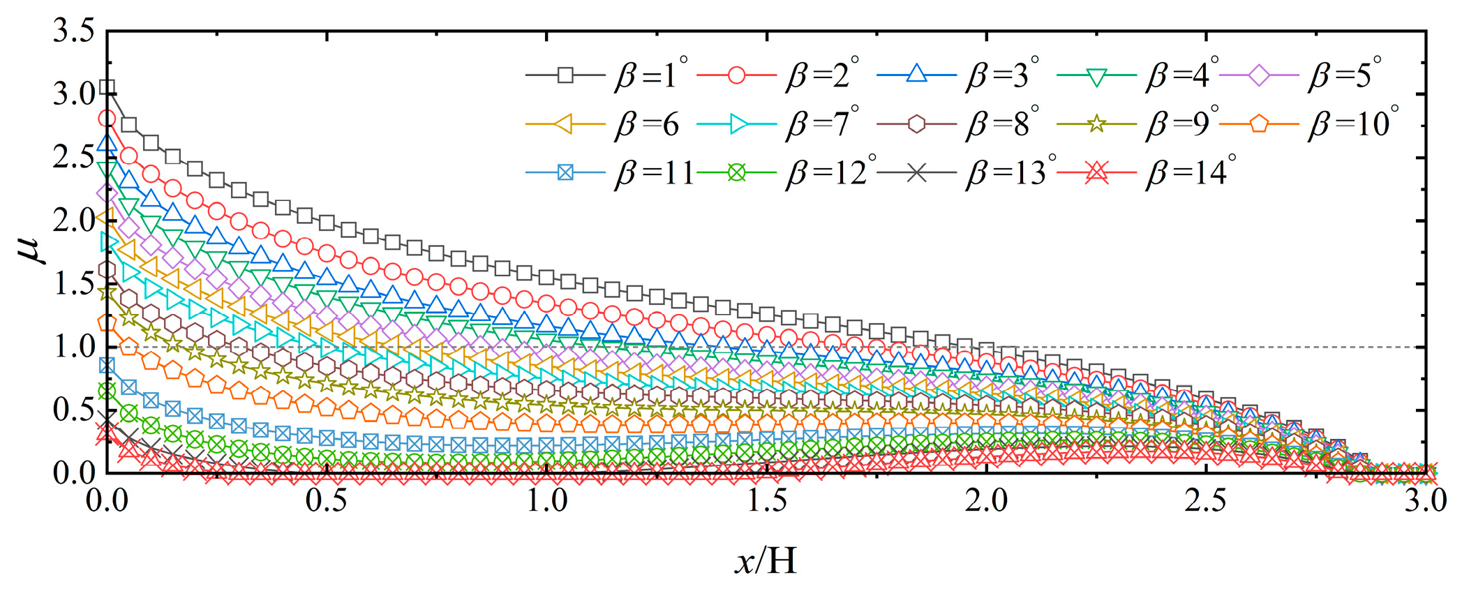
An increase in the slope can effectively reduce the snow accumulation on stepped flat roofs. As the slope increases, the snow removal rate of the roof gradually increases, while the maximum snow depth and snow load shape coefficients subsequently decrease. When the snow load on the roof is less than the ground snow load, there is an optimal slope of the lower roof, making the snow removal rate the maximum and the area of the lower roof the minimum. Finally, considering snow removal efficiency and economic factors, the slope of the lower roof is recommended to be 11°.

Author Contributions

Conceptualization, Z.Z. and W.M.; methodology, Z.Z. and S.L.; software, Z.Z., W.M. and Q.L.; validation, Z.Z., W.M. and Q.L.; formal analysis, Z.Z.; investigation, W.M.; resources, S.L.; data curation, Z.Z.; writing—original draft preparation, Z.Z.; writing—review and editing, Z.Z.; visualization, W.M.; supervision, S.L.; project administration, Q.L.; funding acquisition, W.M. All authors have read and agreed to the published version of the manuscript.

Funding

This research was funded by the National Natural Science Foundation of China, grant number 52278511.

Institutional Review Board Statement

Not applicable.

Informed Consent Statement

Not applicable.

Data Availability Statement

The data presented in this study are available on request from the corresponding author. The data are not publicly available due to privacy.

Conflicts of Interest

The authors declare no conflict of interest. The funders had no role in the design of the study; in the collection, analyses, or interpretation of data; in the writing of the manuscript; or in the decision to publish the results.

References

  1. Li, X.; Zhang, Y.; Li, D.; Xu, Y.; Brown, R.D. Ameliorating cold stress in a hot climate: Effect of Winter Storm Uri on residents of subsidized housing neighborhoods. Build. Environ. 2022, 209, 108646. [Google Scholar] [CrossRef]
  2. Yin, Y.-J.; Li, Y. Probabilistic loss assessment of light-frame wood construction subjected to combined seismic and snow loads. Eng. Struct. 2011, 33, 380–390. [Google Scholar] [CrossRef]
  3. Xie, Z.; Ma, Y.; Ma, W.; Hu, Z.; Sun, G. Comparison of varied complexity parameterizations in estimating blowing snow occurrences. J. Hydrol. 2023, 619, 129291. [Google Scholar] [CrossRef]
  4. Geis, J.; Strobel, K.; Liel, A. Snow-Induced Building Failures. J. Perform. Constr. Facil. 2012, 26, 377–388. [Google Scholar] [CrossRef]
  5. Croce, P.; Formichi, P.; Landi, F. Probabilistic Assessment of Roof Snow Load and the Calibration of Shape Coefficients in the Eurocodes. Appl. Sci. 2021, 11, 2984. [Google Scholar] [CrossRef]
  6. Holicky, M.; Sykora, M. Failures of Roofs under Snow Load: Causes and Reliability Analysis. In Forensic Engineering 2009: Pathology of the Built Environment; American Society of Civil Engineers: Washington, DC, USA, 2009; pp. 444–453. [Google Scholar]
  7. AIJ 2004; AIJ Recommendations for Loads on Buildings. AIJ: Tokyo, Japan, 2014.
  8. EN 1991-1-3: 2003; Eurocode 1: Actions on Structures: Part 1–3: General Actions: Snow Loads. BSI: London, UK, 2003.
  9. GB50009-2012; Load Code for the Design of Building Structures. Ministry of Construction of the People’s Republic of China: Beijing, China, 2012.
  10. American Society of Civil Engineers. Minimum Design Loads and Associated Criteria for Buildings and Other Structures, 7th ed.; American Society of Civil Engineers: Reston, VA, USA, 2017. [Google Scholar]
  11. National Research Council of Canada (Ed.) National Building Code of Canada 2015, 14th ed.; National Research Council of Canada: Ottawa, ON, Canada, 2015.
  12. Tsuchiya, M.; Tomabechi, T.; Hongo, T.; Ueda, H. Wind effects on snowdrift on stepped flat roofs. J. Wind Eng. Ind. Aerodyn. 2002, 90, 1881–1892. [Google Scholar] [CrossRef]
  13. Beyers, J.H.M.; Harms, T.M. Outdoors modelling of snowdrift at SANAE IV Research Station, Antarctica. J. Wind Eng. Ind. Aerodyn. 2003, 91, 551–569. [Google Scholar] [CrossRef]
  14. Zhang, G.; Zhang, Q.; Fan, F.; Shen, S. Field measurements of snowdrift characteristics on reduced scale building roofs based on the size effect study. Structures 2021, 32, 2020–2031. [Google Scholar] [CrossRef]
  15. Jin, Y.; Zhang, Q.; Yin, Z.; Zhang, B.; Liu, M.; Zhang, G.; Fan, F. Experiments on snowdrifts around two adjacent cube models based on a combined snow-wind facility. Cold Reg. Sci. Technol. 2022, 198, 103536. [Google Scholar] [CrossRef]
  16. Liu, M.; Zhang, Q.; Fan, F.; Shen, S. Experimental investigation of unbalanced snow loads on isolated gable-roof with or without scuttle. Adv. Struct. Eng. 2020, 23, 1922–1933. [Google Scholar] [CrossRef]
  17. ASCE 7-16; Snow Loads: Guide to the Snow Load Provisions of ASCE 7-16. American Society of Civil Engineers: Reston, VA, USA, 2017.
  18. Pomeroy, J.W.; Gray, D.M. Saltation of snow. Water Resour. Res. 1990, 26, 1583–1594. [Google Scholar] [CrossRef]
  19. Zhou, X.; Zhang, T. A review of computational fluid dynamics simulations of wind-induced snow drifting around obstacles. J. Wind Eng. Ind. Aerodyn. 2023, 234, 105350. [Google Scholar] [CrossRef]
  20. Zhou, X.; Zhang, T.; Ma, W.; Quan, Y.; Gu, M.; Kang, L.; Yang, Y. CFD simulation of snow redistribution on a bridge deck: Effect of barriers with different porosities. Cold Reg. Sci. Technol. 2021, 181, 103174. [Google Scholar] [CrossRef]
  21. Zhang, G.; Zhang, Y.; Yin, Z.; Zhang, Q.; Mo, H.; Wu, J.; Fan, F. CFD Simulations of Snowdrifts on a Gable Roof: Impacts of Wind Velocity and Snowfall Intensity. Buildings 2022, 12, 1878. [Google Scholar] [CrossRef]
  22. Zhao, L.; Yu, Z.; Zhu, F.; Qi, X.; Zhao, S. CFD-DEM modeling of snowdrifts on stepped flat roofs. Wind Struct. 2016, 23, 523–542. [Google Scholar] [CrossRef]
  23. Naaim, M.; Naaim-Bouvet, F.; Martinez, H. Numerical simulation of drifting snow: Erosion and deposition models. Ann. Glaciol. 1998, 26, 191–196. [Google Scholar] [CrossRef]
  24. Zhou, X.; Zhang, T.; Liu, Z.; Gu, M. An Eulerian-Lagrangian snow drifting model for gable roofs considering the effect of roof slope. J. Wind Eng. Ind. Aerodyn. 2023, 234, 105334. [Google Scholar] [CrossRef]
  25. Zhou, X.; Zhang, Y.; Kang, L.; Gu, M. CFD simulation of snow redistribution on gable roofs: Impact of roof slope. J. Wind Eng. Ind. Aerodyn. 2019, 185, 16–32. [Google Scholar] [CrossRef]
  26. Ma, W.; Li, F.; Zhou, X. An empirical model of snowdrift based on field measurements: Profiles of the snow particle size and mass flux. Cold Reg. Sci.Technol. 2021, 189, 103312. [Google Scholar] [CrossRef]
  27. Zhou, X.; Hu, J.; Gu, M. Wind tunnel test of snow loads on a stepped flat roof using different granular materials. Nat. Hazards 2014, 74, 1629–1648. [Google Scholar] [CrossRef]
  28. Tominaga, Y.; Okaze, T.; Mochida, A. CFD modeling of snowdrift around a building: An overview of models and evaluation of a new approach. Build. Environ. 2011, 46, 899–910. [Google Scholar] [CrossRef]
  29. Zhou, X.; Zhang, Y.; Gu, M. Coupling a snowmelt model with a snowdrift model for the study of snow distribution on roofs. J. Wind Eng. Ind. Aerodyn. 2018, 182, 235–251. [Google Scholar] [CrossRef]
  30. Zhou, X.; Kang, L.; Gu, M.; Qiu, L.; Hu, J. Numerical simulation and wind tunnel test for redistribution of snow on a flat roof. J. Wind Eng. Ind. Aerodyn. 2016, 153, 92–105. [Google Scholar] [CrossRef]
  31. Zhang, Q.; Zhang, Y.; Yin, Z.; Zhang, G.; Mo, H.; Fan, F. Experimental Study of Interference Effects of a High-Rise Building on the Snow Load on a Low-Rise Building with a Flat Roof. Appl. Sci. 2021, 11, 11163. [Google Scholar] [CrossRef]
  32. Zhou, X.; Liu, Z.; Ma, W.; Kosugi, K.; Gu, M. Experimental investigation of snow drifting on flat roofs during snowfall: Impact of roof span and snowfall intensity. Cold Reg. Sci. Technol. 2021, 190, 103356. [Google Scholar] [CrossRef]
  33. Ma, W.; Li, F.; Sun, Y.; Li, J.; Zhou, X. Field measurement and numerical simulation of snow deposition on an embankment in snowdrift. Wind Struct. 2021, 32, 453–469. [Google Scholar]
  34. Kang, L.; Zhou, X.; van Hooff, T.; Blocken, B.; Gu, M. CFD simulation of snow transport over flat, uniformly rough, open terrain: Impact of physical and computational parameters. J. Wind Eng. Ind. Aerodyn. 2018, 177, 213–226. [Google Scholar] [CrossRef]
  35. Richards, P.J.; Norris, S.E. Appropriate boundary conditions for computational wind engineering models revisited. J. Wind Eng. Ind. Aerodyn. 2011, 99, 257–266. [Google Scholar] [CrossRef]
  36. Blocken, B.; Stathopoulos, T.; Carmeliet, J. CFD simulation of the atmospheric boundary layer: Wall function problems. Atmos. Environ. 2007, 41, 238–252. [Google Scholar] [CrossRef]
Figure 1. Roof construction measures [17]: (a) foam blocks on existing roof; (b) inclined roof over accumulation area.
Applsci 13 12109 g001
Figure 2. Mayitas topographic map.
Applsci 13 12109 g002
Figure 3. Measurement site.
Applsci 13 12109 g003
Figure 4. Time history of the wind speed and the friction velocity.
Applsci 13 12109 g004
Figure 5. Outline of the model: (a) model layout; (b) model size.
Applsci 13 12109 g005
Figure 6. Computational domain and grid division.
Applsci 13 12109 g006
Figure 7. Schematic diagram of the dynamic grid.
Applsci 13 12109 g007
Figure 8. Methodological flow diagram.
Applsci 13 12109 g008
Figure 9. Wind environment and temperature in the field measurements.
Applsci 13 12109 g009
Figure 10. The snow deposition on the roofs.
Applsci 13 12109 g010
Figure 11. The snow distribution on the central axis of the roofs: (a) lower roof on the windward side; (b) upper roof on the windward side.
Applsci 13 12109 g011
Figure 12. Snow load shape coefficients for the stepped flat roofs: (a) lower roof on the windward side; (b) upper roof on the windward side.
Applsci 13 12109 g012
Figure 13. Comparisons of the empirical formula in this paper with different countries’ codes.
Applsci 13 12109 g013
Figure 14. Snow accumulation and flow field distribution on stepped flat roofs.
Applsci 13 12109 g014aApplsci 13 12109 g014b
Figure 15. Comparison between the snow simulation and the actual measurement on stepped flat roofs [12,14,22].
Applsci 13 12109 g015
Figure 16. Snow accumulation on the lower roof at different angles.
Applsci 13 12109 g016
Figure 17. Snow removal rate and maximum snow depth on the lower roof at different angles.
Applsci 13 12109 g017
Figure 18. Snow load shape coefficient on the lower roof at different angles.
Applsci 13 12109 g018
Table 1. Parameters of the numerical simulation and field measurements.
ParameterField MeasurementNumerical Simulation
Air density ρ (kg/m3)1.2251.225
Snow density ρs (kg/m3)120~300150
Snow particle diameter ds (μm)165 (Expected value)165
Falling speed wf (m/s)0.2~0.50.2 (h > 0.1 m), 0.35 (h ≤ 0.1 m)
Threshold friction velocity u*t (m/s)0.20.2
Table 2. Calculation settings of the numerical simulation.
Calculation Settings
Computational domain8000 mm (16 L) × 3000 mm (15 H2)
Mesh divisionMinimum grid height: 5 mm. Grid growth rate: 1.1.
Total grid: 30,000. y+: 80.
Mesh quality: the quality and orthogonality are about 1, and the aspect ratio is less than 13.
Inlet boundaryAir phase: Equation (1) and Equations (12) and (13).
Snow phase: Equations (14)~(16).
Ground and model boundaryWall: CS = 2.0, KS = 2 mm.
Outlet boundaryPressure outlet
Upper boundarySymmetry
Table 3. Formulas of snow load shape coefficients in the codes of different countries.
CodeCalculation Formula of μParameter Description
GB50009 2012 [9] μ = L 1 + L 2 / 2 H ( 2.0 μ 4.0 ) x d = 2 H ( 4   m x d 8   m ) L1 is the lower roof span. L2 is the upper roof span. H is the height difference between the stepped flat roofs. xd is the length of the nonuniform snow distribution. μb is the snow uniform distribution coefficient. μw is the drift coefficient. μs is the slide coefficient. Ca and μi are the shape coefficients of the snow load. Ce is the exposure coefficient. Ct is the temperature coefficient. Cs is the roof slope coefficient. γ is the weight density of snow. Is is the building importance factor. lc is the characteristic length of stepped flat roofs. hb is the uniform snow thickness. hd is the snowdrift thickness. hc is the height difference from the uniform snow surface to the upper roof. Sb is the uniformed snow load.
ASCE 2017 [10] μ = γ h d + h b S 0 h d I s = 0.43 L 1 3 S 0 + 10 4 1.5 h d h c h b = S b / γ γ = 0.13 S 0 + 14 γ 30 lb / ft 3 x d = 4 h d h d h c 4 h d 2 / h c h d > h c x d 8 h c
EN 1991-1-3 2003 [8] μ = μ i C e C t μ 2 = μ w + μ s μ w = b 1 + b 2 / 2 h μ w γ H / S 0 μ s = 0 α < 15 0.5 μ 1 α 15 x d = 2 H 5   m x d 15   m
NBCC 2015 [11] μ = I s μ b C e C s C a μ b = 0.8 l c 70 C e 2 1 C e 1 1 0.8 C e exp l c C e 2 70 100 l c > 70 C e 2 C a = C a 0 C a 0 1 x / x d 0 x x d 1.0 x > x d x d = 5 μ b S 0 γ C a 0 1 C a 0 = min β γ H μ b S 0 , F μ b
AIJ 2004 [7] μ = μ b + μ w + μ s μ s = 0 α < 10 μ b α 25
Table 4. Comparison of the maximum snow load shape coefficients and the unbalanced length of snow.
Code or EquationMaximum μDimensionless Unbalanced Length (x/H)
AIJ12
ASCE20.5
NBCC2.71
EN2.52
GB2.52
Equation (20)3.441.6
Equation (21)3.442
Disclaimer/Publisher’s Note: The statements, opinions and data contained in all publications are solely those of the individual author(s) and contributor(s) and not of MDPI and/or the editor(s). MDPI and/or the editor(s) disclaim responsibility for any injury to people or property resulting from any ideas, methods, instructions or products referred to in the content.

