A Comparative Study of a Hybrid Experimental–Statistical Energy Analysis Model with Advanced Transfer Path Analysis for Analyzing Interior Noise of a Tiltrotor Aircraft

Abstract

The excessive noise present within an aircraft cabin during flight operations constitutes a notable origin of fatigue, stress, and communication impediments for both pilots and passengers. Ensuring the comfort, well-being, and safety of passengers and crew members necessitates the accurate anticipation of noise levels. This study concerns the computation of structure-borne noise levels within the cabin of a tiltrotor aircraft. This investigation employed two distinct methodologies: advanced transfer path analysis (ATPA) and statistical energy analysis (SEA). To assess the results obtained with the ATPA approach, the acquired outcomes were compared with empirically measured sound pressure levels during airplane mode operations. The contributions of air-borne and structure-borne noises were calculated with the ATPA methodology. On the other hand, the structure-borne noise was calculated with a hybrid experimental–SEA model with ACTRAN software, and its results were compared with those of the ATPA method. The results show a good agreement between these methods at high frequencies, while at low frequencies, certain adjustments or modifications to the SEA model are necessary to predict the noise levels.

1. Introduction

A vibroacoustic analysis is an essential step in the design of aircraft, trains, cars, and industrial machines. It ensures the performance, quality, and safety of products and systems. Additionally, vibroacoustic analysis can be used to identify sources of noise and vibration in structures and systems. By comprehending the fundamental reasons for noise and vibrations, it is possible to develop efficient control strategies such as active noise cancelation to mitigate them.

When developing modern aircraft designs, it is crucial to take into account the aircraft’s noise and vibration features. Tiltrotor aircraft, known for their vertical take-off and landing capabilities, have gained popularity in both military and civilian applications. However, this distinctive configuration introduces novel challenges related to noise generation [1,2,3]. In recent years, some studies have proposed new methods or designs to reduce the structure-borne noise inside an aircraft or helicopter. For instance, Wang et al. [4] proposed a novel periodic mono-material strut with geometrical discontinuity for the main gearbox of a helicopter that reduces the structure-borne noise inside the cabin. Rostami et al. [5] focused on the possibility-based design optimization (PBDO) method to optimize an electric vertical take-off and landing aircraft in the conceptual design phase. Misol [6] considered the use of active trim panels for interior noise reduction instead of active fuselage structures (with actuators on fuselage panels or frames).

In order to mitigate the interior noise of an aircraft, it is important to predict the interior noise properly. Over the past few years, numerous approaches such as statistical energy analysis (SEA) and advanced transfer path analysis (ATPA) have been developed to facilitate the characterization of the vibroacoustic behavior of structures and systems.

The ATPA technique is used to identify the transmission paths of vibrations and noise in a system and to quantify the contributions of different components [7,8]. ATPA involves measuring the vibration and noise levels at various points in a system and then using the theory of transfer matrices to determine the contributions of each path to the overall response [9].

In a network of interconnected nodes, a path between node i and node j is recognized if they are directly connected. In the context of a vibroacoustic system, these nodes represent subsystems, and signals (vibrations or acoustic pressure) are utilized to analyze and explore these paths. It is essential to differentiate between a path from i to j and a contribution from i to j. A contribution indicates the signal amount reaching node j due to an excitation at node i. This signal, however, can be transmitted through various paths from i to j, irrespective of the direct connection between the two nodes. Thus, contributions describe inputs and outputs, while paths provide a description of the system’s topology. The objective is consistently to characterize the response of every subsystem, which is quantified in terms of the acceleration of a vibrating component or the acoustic pressure within a specific area of concern, triggered by a distinct excitation.

When considering the studied system as a black box containing n inputs and m outputs interconnected within, ATPA can forecast the individual contribution of each input to every output. It achieves this by decomposing the output signal into distinct contributions originating from each input signal. Additionally, ATPA can effectively analyze the interconnections between input and output signals within the black box, revealing the inherent structure of the mechanical system, including the paths through which signals propagate [3]. Consequently, when a comprehensive examination of the mechanical system is required, ATPA proves to be a valuable tool.

On the other hand, statistical energy analysis (SEA) is a well-known method to analyze the flow of acoustic and vibrational energy in a complex structure. This method is particularly beneficial for predicting the noise and vibrational behavior of structures that have many degrees of freedom and multiple energy pathways at mid to high frequencies. The SEA method can analyze vibroacoustic behavior at high frequencies, and it has found applications in various industries, including the automotive, aerospace, construction, and marine industries.

The method involves dividing a complex system into a series of subsystems or components. Each component is then modeled as a separate entity, with its own set of properties such as mass, stiffness, and damping. The interactions between components are through junctions that provide energy flow paths [10]. These paths are used to predict the energy transfer between the components and the resulting response of the entire system [11].

The utilization of a simulation model enables the prediction of the vibroacoustic behavior of a system, thereby contributing to the reduction in development cycles and design expenses, as well as facilitating the evaluation of the impact of component performance on vibroacoustic comfort. To this end, in this study, the interior noise of a cabin was calculated using the virtual statistical energy analysis (VSEA) module of ACTRAN, which uses the eigenvalues and mode shapes of a finite element (FE) vibroacoustic model. The objective of this study was to compare the results of the VSEA simulation with the results provided via the ATPA measurements.

The subsequent sections provide a comprehensive overview of the ATPA and SEA theories, followed by explanations of the ATPA campaign test and the SEA simulation using ACTRAN software. In Section 4, the results of these two methods are presented, and they are compared.

Finally, the findings of this study are summarized in Conclusions.

2. Theory

2.1. Advanced Transfer Path Analysis Method (ATPA)

ATPA characterizes the topology of a mechanical system to find out the vibroacoustic paths and the contributions of the system’s components, called subsystems, to the noise at any receiver. This method works based on the coefficients of the global transfer matrix ${\mathbf{T}}^G$, which are defined as [7,12]

$${\mathbf{T}}_{ij}^G=\frac{x_j}{x_i}$$

(1)

where $x_j$ is the signal at node j, whilst an excitation is applied at node i. Typically, $x_j$ is an acceleration, a rotation acceleration, or a pressure.

The global transfer matrix is related to the contributions of the subsystems. On the other hand, the direct transfer matrix ${\mathbf{T}}^D$ is another coefficient that is used to characterize paths. The coefficient ${\mathbf{T}}_{ij}^D$ has information about the path between the nodes i and j and is defined as

$${\mathbf{T}}_{ij}^D=\frac{x_j}{x_i}$$

(2)

with all the nodes other than i and j blocked. The direct transfer matrix can also be defined from any of the nodes to an external target point T where some output of interest is defined and controlled.

$${\mathbf{T}}_{iT}^D=\frac{p_T}{x_i}$$

(3)

In this case, $p_T$ can be the pressure at the target point T when excitation is applied. ${\mathbf{T}}_{iT}^D$ is calculated as the relation between the pressure at the target T and the excitation at node i, with all the nodes j ≠ i blocked. The total pressure at the target point T is defined as

$$p_T=\sum _{i=1}^N{x}_i{\mathbf{T}}_{iT}^D+p_T^e$$

(4)

where $p_T$ is a signal in the target, $x_i$ is the measured signal in subsystem i (i.e., the acceleration of a vibrating panel), ${\mathbf{T}}_{iT}^D$ is the direct transfer function between subsystem i and the target, and N is the number of subsystems into which the mechanical system has been divided. In Equation (4), $p_T^e$ is the direct field of the signal that arrives at T due to an external excitation when all the N nodes are blocked.

In addition, a relationship between the global transfer defined in Equation (1) and the direct transfer defined in Equation (3) can be obtained.

$$\sum _{j=1}^N{\mathbf{T}}_{ij}^G{\mathbf{T}}_{jT}^D={\mathbf{T}}_{iT}^G\hspace{1em}for i=1,2,\dots ,N$$

(5)

The characterization of the paths is then reduced to the mathematical problem of determining the coefficients ${\mathbf{T}}_{iT}^D$. This can be carried out, for example, using the solution of the linear system of just N equations like Equation (5) (for the case of exactly N executions of the experiment).

In ATPA, three types of subsystems are defined: structural, panel, and aerial subsystems. Structural subsystems are those that link the vibroacoustic source to the target through structural linking points (like a damped or rigid joint). Panels refer to the system’s components that radiate noise and contribute to the noise perceived at the target. Aerial subsystems, like leaks or holes, are elements through which only air-borne transmission paths can be defined.

ATPA can synthesize the noise at a target $T$ as a sum of noise contributions. In this regard, the total contribution from a set of panel or structural subsystems at a target position $T$ is defined via Equation (6).

$$p_{syn,T}\left(\omega ,t\right)=\sum _{i=0}^N{a}_i\left(\omega ,t\right)T_{i\to T}^D\left(\omega \right)=\sum _{i=0}^N{p}_i\left(\omega ,t\right)$$

(6)

where $i$ corresponds to a panel or a structural subsystem, $a_i\left(\omega ,t\right)$ is the acceleration in subsystem $i$, and $T_{iT}^D\left(\omega \right)$ is the direct transfer function from subsystem $i$ to target $T$. In this equation, $p_i\left(\omega ,t\right)$ is the noise contribution of subsystem $i$ at the target location $T$.

Furthermore, the method allows for splitting the panel noise into structure-borne and air-borne noise. The structure to panel contribution is obtained via a two-step calculation:

$$a_{syn,i}\left(\omega ,t\right)=\sum _{j=0}^M{a}_j\left(\omega ,t\right)T_{ji}^D\left(\omega \right)$$

(7)

And

$$p_{struct,i}\left(\omega ,t\right)=a_{syn,i}\left(\omega ,t\right)T_{iT}^D\left(\omega \right)$$

(8)

where $i$ corresponds to a panel subsystem, $j$ corresponds to a structural subsystem, $a_{syn,i}\left(\omega ,t\right)$ is the synthesized acceleration in panel $i$ due to structural excitation, and $p_{struct,i}$ is the synthesized pressure at target $T$ due to the structural excitation of the panel. This corresponds to the structure-borne noise contribution of the panel.

The air-borne contribution of each panel is calculated as the subtraction of the total panel contribution and the structural panel contribution.

2.2. Statistical Energy Analysis (SEA)

In the SEA method, the power balance of a subsystem depends on the input power, transfer power between subsystems, and dissipated power through the subsystem. Equation (9) describes the power balance of subsystem $i$.

$$P_{i,input}=P_{i,dissipated}+P_{ij}$$

(9)

where $P_{i,input}$ is the input power of the subsystem, $P_{i,dissipated}=\omega {\eta }_i{E}_i$ is the dissipated power within the subsystem, which depends on the internal damping loss factor ${\eta }_i$ of the subsystem, and $P_{ij}$ is the transfer of power between subsystems. This latter parameter depends on the modal energy of each subsystem as well as the coupling loss factors between subsystems $i$ and $j$. The power transfers from a subsystem with higher modal energy to one with lower modal energy [13]. This parameter for a system of $N$ subsystems is defined as

$$P_{ij}=\sum _{j=1}^N\omega ({\eta }_{ij}{E}_i-{\eta }_{ji}{E}_j)$$

(10)

where $\omega$ is the angular frequency, ${\eta }_{ij}$ is the coupling loss factor, and $E_i$ and $E_j$ are the total subsystems’ energy. In SEA, it is assumed that in the narrowband, the modal energies of all modes are the same. Based on this assumption, there is a reciprocal relationship between subsystems considering their coupling loss factors and their modal densities:

$${\eta }_{ij}{n}_i={\eta }_{ji}{n}_j$$

(11)

where $n_i$ and $n_j$ are the modal densities of subsystem $i$ and $j$, respectively. Considering Equations (10) and (11), the transfer power between subsystems can be written as

$$P_{ij}=\sum _{j=1}^N\omega {\eta }_{ij}{n}_i(\frac{E_i}{n_i}-\frac{E_j}{n_j})$$

(12)

By substituting Equation (12) into Equation (9), the power balance of subsystem $i$ can be written as

$$P_{i,input}=\omega {\eta }_i{E}_i+\omega \sum _{j=1}^N\omega {\eta }_{ij}{n}_i(\frac{E_i}{n_i}-\frac{E_j}{n_j})$$

(13)

This power balance equation is used in a matrix solution format to determine the energy vector.

In this study, the virtual SEA method was utilized for analyzing the tiltrotor based on the VSEA module of ACTRAN. In Section 3.2 the methodology of using this method is explained in detail.

3. Methodology

3.1. ATPA

This section outlines the application of the ATPA methodology to define the noise level in the tiltrotor aircraft. It begins by defining the area of study and then proceeds to list the subsystems and targets involved in the assessment. Finally, a detailed description of the ATPA test is provided.

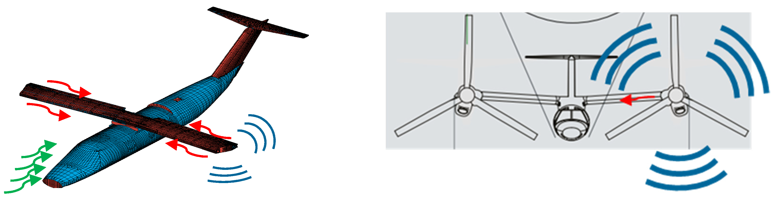
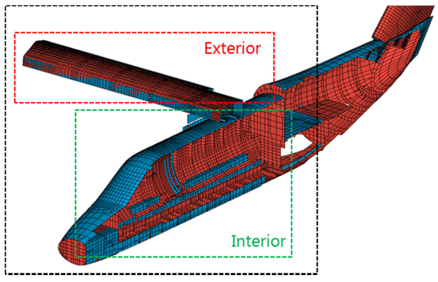
3.1.1. Area of Study

The area of study is defined according to the identification of the relevant noise sources and the receiver. Information about noise contributions and transmission paths is required to be determined for at least two locations inside the aircraft cabin (the pressurized area), which establishes this area as the main area of study.

In the tested configuration, the expected main sources are the engine and the propeller, located at the end of the wings. Figure 1 schematically shows the air-borne and structure-borne noise transmission of these sources. Another important noise source is the aerodynamic contribution, represented in green, which may only be assessed if in-flight operation conditions are tested.

Considering the mentioned sources, the main area of study (the pressurized cabin) is complemented with external controlled parts, which consist of several structural points at the wing’s connection to the fuselage and motor propeller assemblies. The complete area of study is shown in Figure 2.

3.1.2. Relevant Structural Linking Points

A preliminary study of the relevant structural connection points that are found throughout the path from the main vibroacoustic source (rotor) to the cabin has been carried out. This path includes the engine/rotor connections, the transmission shaft connections (saddles) to the wing, and the wing–fuselage connection. This study will represent an extensive definition of possible structural subsystems to be considered for the test. From all these, a simplified list is considered the final set of structural subsystems for the ATPA test.

3.1.3. List of Subsystems and Targets

The final set of subsystems chosen for the test is described as follows. It includes two types of subsystems: cabin interior panels and structural points.

• Interior panels: The list of panel subsystems is composed of different elements inside the study area, that is, the pressurized cabin of the aircraft. On one side, individual elements such as windows or doors are considered as single subsystems. On the other side, larger areas such as the floor or the ceiling are divided into smaller areas, each one of them being a subsystem, represented with an accelerometer at a certain location within the area, in the normal direction to the panel.
• Structural subsystems: The definition of the structural points is based on the study of relevant structural points. From the structural connections, the essential ones are the wing–fuselage connection points, and they are instrumented with a triaxial accelerometer, explained in Section 3.2.2.

Moreover, two receivers (targets) are defined for the ATPA test. These points are the locations where the information on noise transmission paths and contributors is calculated. The target locations are as follows:

• Target 1: The pilot seat, at ear height.
• Target 2: A passenger seat, at ear height.

3.1.4. ATPA Test Description

The instrumentation is composed of accelerometers and microphones, which represent subsystems and targets, respectively.

• Subsystems: One accelerometer per subsystem is required.
• Targets: One microphone per target is required.

The ATPA experimental procedure is composed of two different tests: static and dynamic tests.

• Static test:

Static tests consist of an impact test at each of the considered subsystems. The impacted subsystem is called the reference subsystem. The response is measured in all other subsystems, including the targets. They are called response subsystems. The measurement functions are the so-called global transfer functions (GTFs or T^Gs).

With this impact, the transmissibility between the subsystems (acceleration over acceleration) and between each subsystem and the target (acceleration over pressure) can be obtained. Also, the transfer functions of acceleration over applied force (impact) and pressure over force are measured.

2.

Dynamic test:

The dynamic test consists of recording the acceleration and acoustic pressure signals at the same exact locations where the static test responses were measured, including the target, while the tiltrotor is in operation.

3.2. SEA Model

As previously introduced, SEA is an energy-based method to predict the response of a dynamic system to input power. This method is commonly utilized to represent the high-frequency vibrational dynamics of complex systems in an averaged or approximate manner [14]. In the SEA approach, several assumptions are considered in the development of a model. These assumptions include the following [15]: (1) The input power is white noise, which has a broadband spectrum, and (2) the subsystems are weakly coupled. This means the excited subsystem has a higher response than other subsystems. (3) The subsystems are assumed to be uncoupled.

Bearing in mind these assumptions, this study modeled a fuselage section of a tiltrotor aircraft using ACTRAN, within the VSEA module. The power injection method (PIM) is employed within this module to virtually excite all modes of a subsystem [16,17].

To predict the interior noise of the model, a range of inputs is essential. These inputs encompass the mesh file representing the structure and cavity, the mode shapes of both the structure and cavity, the stiffness and mass matrices of the model, as well as the boundary conditions applied to the system. The subsequent sections outline the inputs utilized in the modeling procedure.

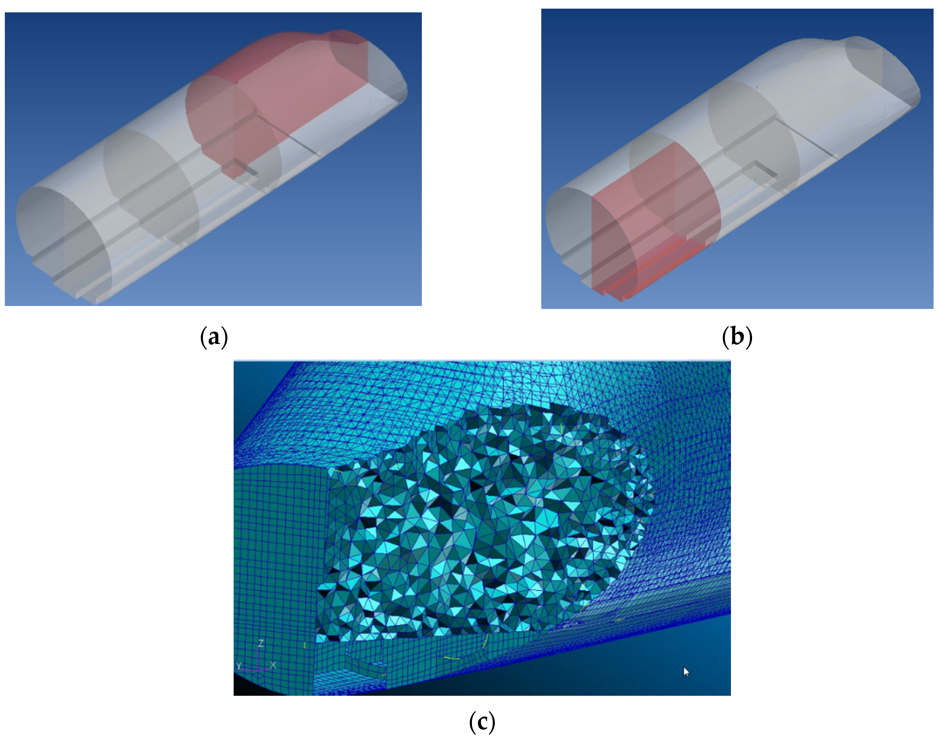
3.2.1. Mesh Elements and Subsystem Definition

To generate a mesh for the structural framework of the aircraft, a mixture of two-dimensional plate elements and one-dimensional beam elements is employed. In the model, these elements are grouped into different subsystems to predict the noise contributions from various parts of the structure. These subsystems are the same as the ones considered in the experimental ATPA measurements. The model includes 33 subsystems. Figure 3 represents four subsystems of the model and mesh elements.

In addition, the aircraft’s cavity is meshed using Nastran’s Tetra-10 3D element type. In accordance with the general rule, the size of the elements is determined by ensuring that a minimum of six nodes are incorporated within the shortest wavelength of interest. This criterion allows for the accurate calculation of the system’s mode shapes. To ensure an accurate representation of the mode shapes up to 1250 Hz, the maximum element size within the cavity is determined as 0.04 m.

The cavity is partitioned into six subdivisions, each representing a distinct subsystem within the model. These subsystems are coupled with each other and with the structural subsystems. Figure 4 illustrates two cavity subsystems and the mesh elements of the cavity. The boundaries of the fluid topology precisely follow those defined by the structural mesh.

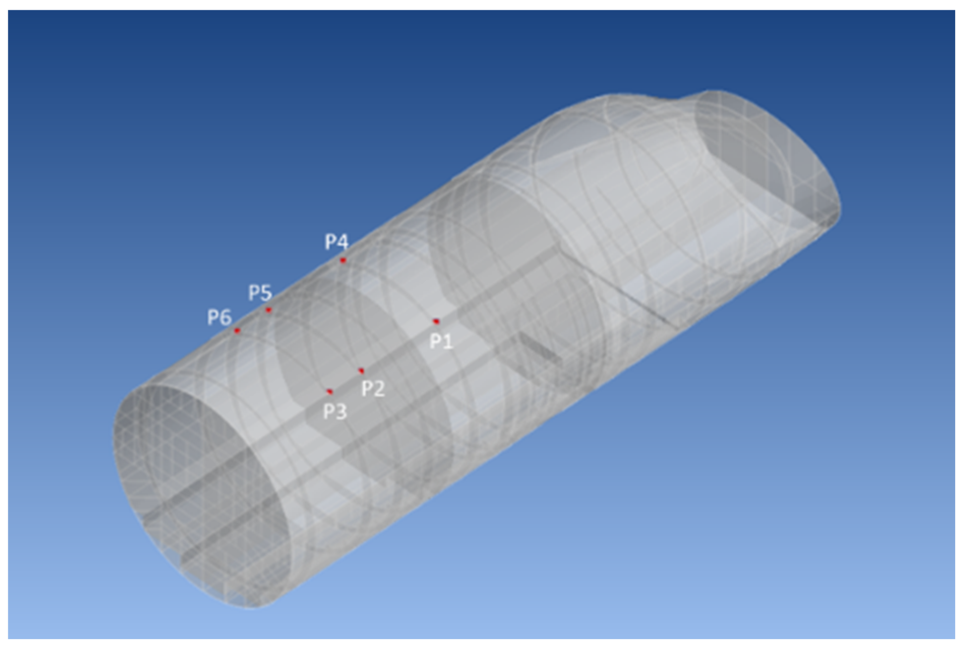
3.2.2. Boundary Conditions

The force applied to the fuselage during the operation should be considered in the SEA model. This force is employed to predict the interior noise levels within the cabin. To this end, the operational forces applied to structural linking points from the wings to the fuselage of the tiltrotor are computed based on classical transfer path analysis and within the matrix inversion procedure. The operational forces applied to structural linking points from the wings to the fuselage are computed at six points. Figure 5 shows these linking points.

The forces are determined via experimental data. This procedure necessitates the following information:

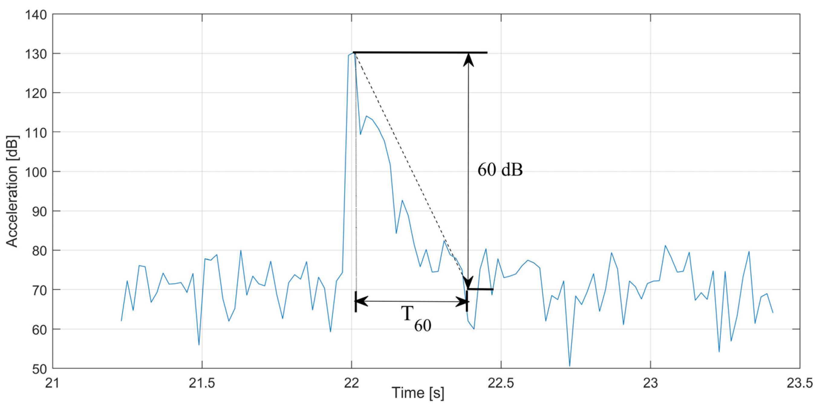
• The frequency response functions (FRFs) at the linking points. These data are provided during experimental measurements by impacting with an instrumented hammer the linking points between the wings and fuselage.

  $$H=\raisebox{1ex}{$a$}\!\left/ \!\raisebox{-1ex}{$F$}\right.$$

  (14)
  $H$ is the accelerance FRFs, $a$ is the acceleration, and $F$ is the impact force.
• The data on accelerations in operating conditions are measured at the same structural points as during the operational conditions.

A system of linear equations with an equal number of equations and unknowns typically provides a unique solution; however, it can introduce substantial inaccuracies [18]. In other words, minor adjustments in the input data can result in significant variations in the obtained results. There are several options available to enhance the estimation of the forces, such as generating an over-determined system of equations. This can be achieved by adding extra equations using the information recorded on some of the internal panels of the tiltrotor when exciting the structural points. Equation (15) represents a system of equations for an over-determined system:

$$\left[\begin{array}{ccc}\begin{array}{c}\frac{a}{F_1}\\ ⋮\\ \begin{array}{c}\frac{a_n}{F_1}\\ \frac{a_{n+1}}{F_1}\\ \begin{array}{c}⋮\\ \frac{a_{n+p}}{F_1}\end{array}\end{array}\end{array}& \dots & \begin{array}{c}\frac{a}{F_n}\\ ⋮\\ \begin{array}{c}\frac{a_n}{F_n}\\ \frac{a_{n+1}}{F_1}\\ \begin{array}{c}⋮\\ \frac{a_{n+p}}{F_n}\end{array}\end{array}\end{array}\end{array}\right]\left[\begin{array}{c}{F}_1\\ ⋮\\ F_n\end{array}\right]=\left[\begin{array}{c}{a}_1\\ ⋮\\ a_n\\ a_{n+1}\\ ⋮\\ a_{n+p}\end{array}\right]$$

(15)

where n is the number of structural points, and p is the number of panels used to over-determine the system of equations. Equation (15) is used to calculate the operational forces, and they are used as the boundary conditions of the model.

3.2.3. Mechanical Properties

The mass/stiffness matrices and the mode shapes of the model are two properties that are required for an SEA analysis. In this study, these properties are obtained using the dynamic reduction technique in Nastran.

On the other hand, the damping loss factor (DLF) is another mechanical property of the system that represents the ability of a material or structure to dissipate mechanical energy in the form of vibrations. In this study, the damping loss factors of both the aircraft’s panels and cavity are computed using the decay rate method (DRM) and via the impact test performed during the experimental measurements. This method is based on measuring the response at a mounted accelerometer to a force impulse impacted with a hammer on the panel [19]. This method relies on the force impulse applied with an impact hammer and the corresponding response measured with accelerometers, which are randomly positioned on the panel. In this method, it is essential to conduct an adequate number of measurements to obtain a meaningful average that holds statistical significance. In this study, five measurements are carried out for each panel, and the average damping loss factors (DLFs) of panels with the same material are utilized.

The principle of this approach is to identify the time decay needed for an impact response to reduce by 60 dB compared with the initial peak value (Figure 4). When the dynamic range does not allow for a decay of 60 dB, a lower range of dB might be used. The damping is defined as

$$\eta =\frac{\overline{\alpha }}{\omega }$$

(16)

where $\omega$ is the angular frequency, and $\overline{\alpha }$ represents the average of $\alpha =\Delta \ln \left(\mathrm{Acceleration}\right)/T_{60}$ from several impacts. Figure 6 shows the acceleration of a subsystem that is impacted by an impulse force and the time decay.

3.2.4. Extended Solution

In the high-frequency range, however, the behavior of a structure becomes energetic. As frequency increases, the mode shapes occur closer and closer together, which increases the modal density. Modal density is one of the main parameters in the SEA model. It quantifies the energy storage capacity of a vibration system. As the modal density increases, the calculation of mode shapes becomes a more time-intensive procedure, subsequently making the calculation of the interior sound pressure computationally expensive. In this study, the extended solution method of ACTRAN was employed for the calculation of interior noise from 1250 Hz to 4000 Hz. In this solution, SEA matrices are computed based on extrapolated quantities.

4. Results and Discussions

4.1. Operational Force

As mentioned in Section 3.2.2, the operational forces applied to the linking joints are calculated from the acceleration of those points in the operational mode. These data are collected with tri-axial accelerometers, and the modulus of acceleration is calculated for each point. Figure 7 illustrates the resultant operational force spectra acting on the linking points. There are three linking points on each side of the aircraft. These points connect the wings to the fuselage. The locations of these points are shown in Figure 5.

This figure shows that the forces applied from the wings to the fuselage are similar on both sides of the tiltrotor. These forces’ spectra are used as the boundary conditions in the SEA model to define the interior noise levels at the target points.

4.2. Results of ATPA

Figure 8 compares the experimentally measured noise level at Target 1 with the noise level computed using the ATPA methodology at the same location. Additionally, the figure delineates the contributions of structure-borne and air-borne noise components separately.

As shown in this figure, the noise level computed using ATPA closely aligns with the measured noise pressure. The figure also illustrates that air-borne noise is the main contributor to the overall noise. The structure-borne noise component is higher in the range of 160–1000 Hz compared with the rest of the frequency range.

The noise pressure at Target 2 is calculated with the same method. Figure 9 illustrates a comparison between the sound pressure levels obtained using ATPA and direct measurements. The measured noise level is well synthesized with the ATPA method, except in the range between 200 and 300 Hz, where a gap between the measurement and synthesis is observed. This might be due to a modal behavior that cannot be reconstructed with the ATPA energetic approach used in this work.

As in Target 1, the results show that air-borne noise significantly outweighs structural-borne noise, across the whole frequency range.

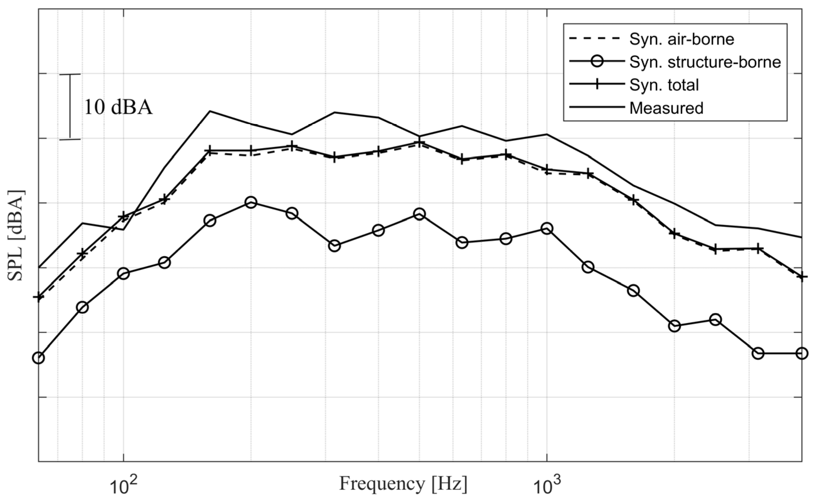
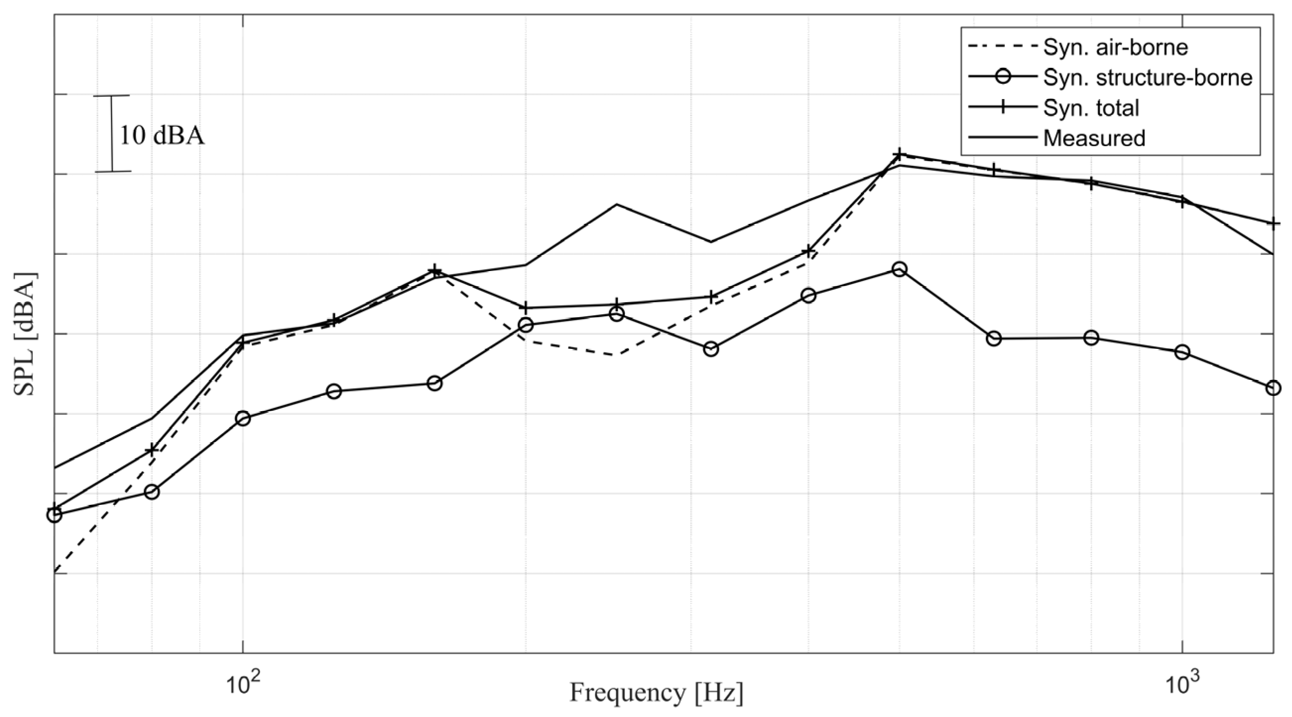
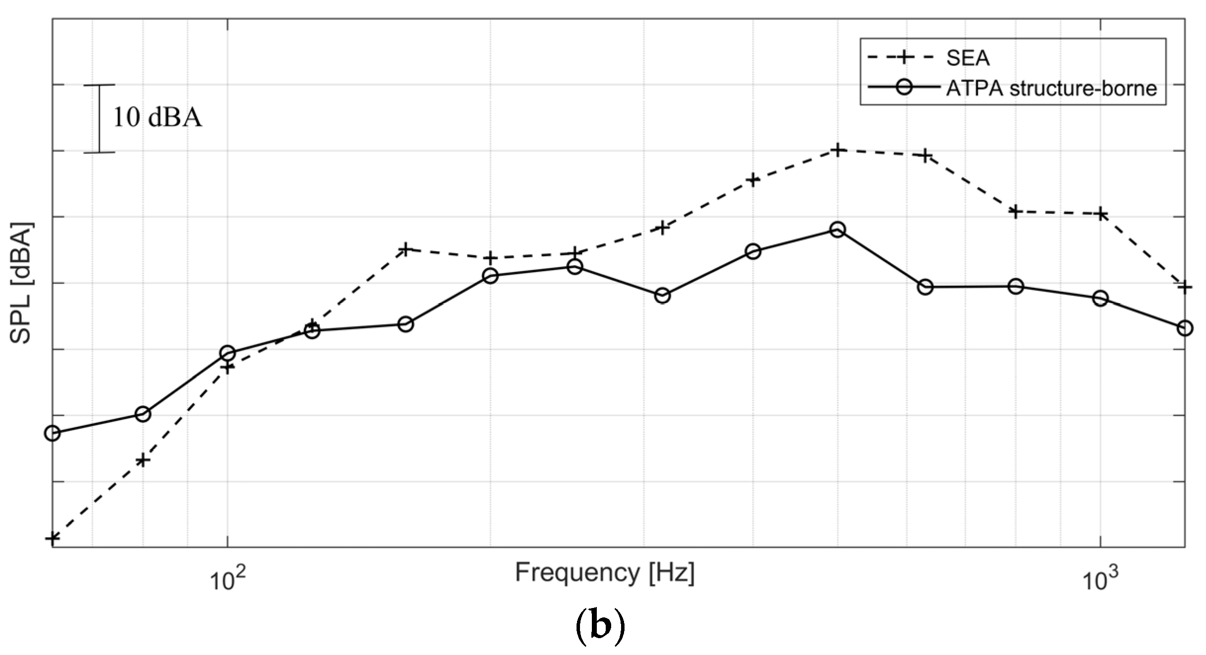
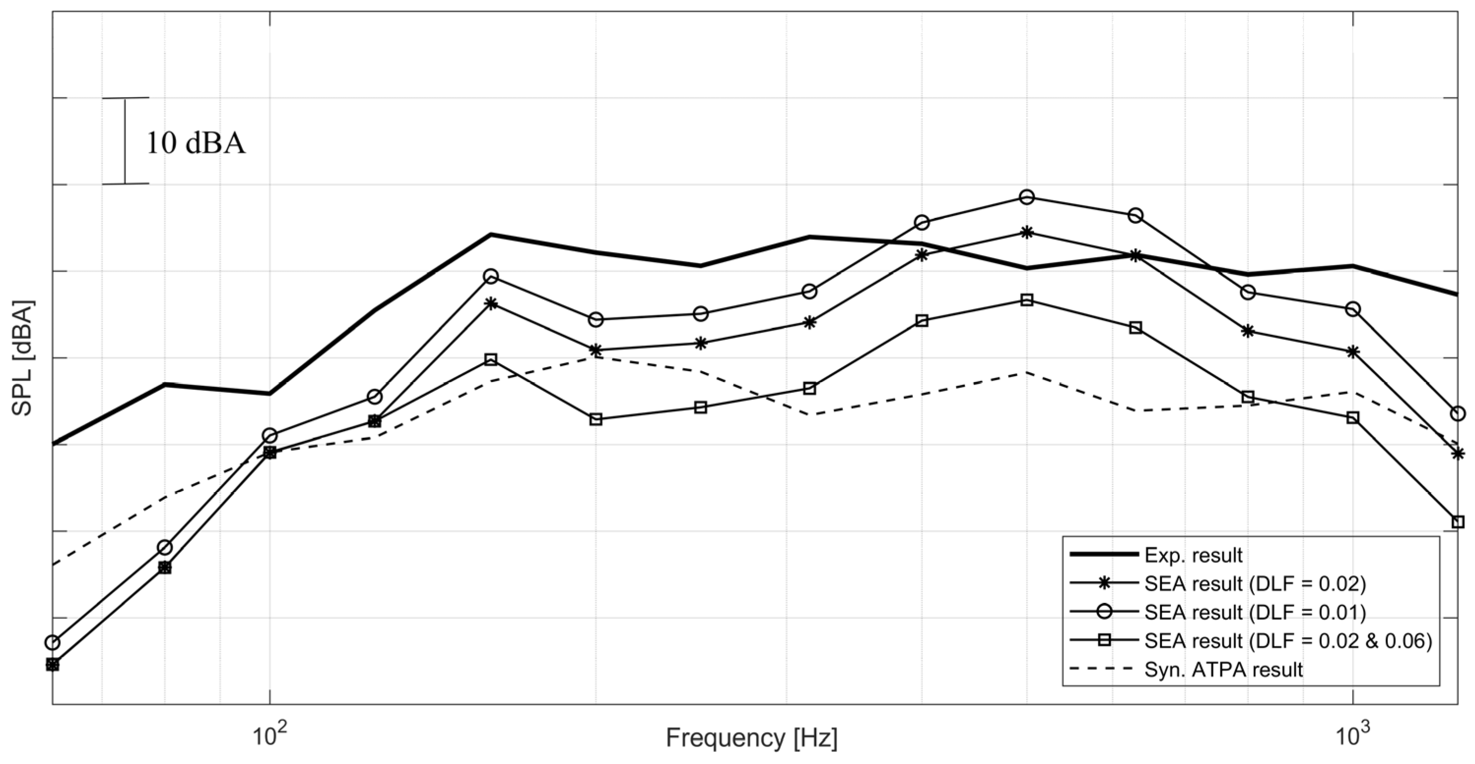
4.3. Results of SEA vs. ATPA

Air-borne noise was omitted from the SEA model due to the absence of dedicated testing focused solely on the air-borne path, such as knowledge about the transmission loss of the panels [20]. In this context, a comparison is drawn between the results of the SEA model and the structure-borne noise analysis conducted using ATPA.

Figure 10 compares the noise level prediction of the SEA approach with the structure-borne noise contribution calculated using ATPA.

As shown in Figure 10, the ATPA and SEA methods predict the same trend for noise pressure, although there are some discrepancies between the results. There are various parameters in an SEA analysis that affect the output, such as the complexity of the model’s geometry, the material properties, and the boundary conditions used to describe the interactions between the structure and the cavity. If the boundary conditions are not well-defined or are not representative of the actual environment, the predicted sound pressure levels may not match the measured values. Also, the SEA model may not accurately capture the effects of non-uniformities, irregularities, or discontinuities in the structure. In particular, the interior of the aircraft was in green mode, with visible ribs and some elements (like a bulky emergency exit at the rear part of the cabin), which were not present in the model.

Furthermore, the accuracy of SEA predictions is strongly influenced by the acoustic damping loss factor, which affects the dissipation of energy in the cavity. In this study, the acoustic damping factor was obtained from impact tests on panels, but a more reliable approach would have been to excite the cavity rather than a panel. This is further discussed in Section 4.5.

4.4. Extended Solution

The virtual SEA model can be used to extend the prediction of noise level up to 4 kHz using the ACTRAN extended solution [21,22]. Figure 11 displays the noise level prediction obtained up to 4000 Hz. For this simulation, the structure and cavity mode shapes are achieved for up to 1250 Hz with the FEM model. The extended solution predicts the higher frequency mode shapes and computes the noise pressure levels.

Figure 11 depicts how this solution anticipates a noise trend consistent with the calculations derived from ATPA, particularly at high frequencies. Discrepancies between the model outcomes and ATPA results can potentially be attributed to the underlying assumptions of the SEA techniques. Furthermore, the SEA results are acquired via mode shapes sourced exclusively from the range of 900 Hz to 1250 Hz (via interpolation). For higher frequencies, an extrapolation technique is applied (referred to as the extended solution).

4.5. Effect of Acoustic Damping on the Interior Noise

The acoustic damping inside the cavity is an important parameter that affects the noise level at the targets. We investigated the effect of the acoustic damping loss factor on the noise level received at Target 1.

Figure 12 displays the sound pressure level at the position of Target 1 with different acoustic DLFs.

The depicted figure highlights the substantial impact of acoustic damping on the received noise at a receiver. Furthermore, the figure indicates that for frequencies exceeding 200 Hz, employing an acoustic damping factor (DLF) of 0.06 yields results that closely approximate those obtained using ATPA. The average difference between the results of ATPA and SEA in one-third of octave bands (in the frequency range of 63 Hz to 1250 Hz) is 9.4 dB, but it can be significantly improved with an adjustment of the acoustic DLF, resulting in an average of 5.4 dB (see Figure 12). On the other hand, the differences between the overall sound pressure levels calculated using the ATPA and SEA methods with an adjusted DLF (in the same frequency range) are 4.1 dB for Target 1 and 5.4 dB for Target 2.

It is worth noting that the acoustic DLF values were computed from impact tests on panels as opposed to acoustic cavity excitation, which might have led to a more precise determination of this parameter.

5. Conclusions

This research undertook a comprehensive investigation into predicting interior noise in a tiltrotor aircraft using two methods: advanced transfer path analysis (ATPA) and statistical energy analysis (SEA). The results presented in this study confirm the reliability of the well-known ATPA method as a valuable tool for characterizing the interior noise in an aircraft, as the noise levels calculated using ATPA match with those obtained via experimental measurements at two target points within the cabin. Moreover, this study involved a comparison between the ATPA structure-born noise levels and the results from an aircraft SEA model.

For this comparison, this research introduced a hybrid experimental–SEA model to predict structural-borne noise. The model utilizes input data derived from the ATPA campaign test and a finite element model of the aircraft. In this model, ACTRAN is used for the SEA calculations.

Overall, both ATPA and the hybrid experimental–SEA model exhibited a consistent trend in structural-born noise prediction. However, a noteworthy average difference of 9.4 dB was observed between the two methods in the one-third octave band noise range of 63 Hz to 1250 Hz. Importantly, this disparity could be significantly reduced via the adjustment of the acoustic damping loss factor (DLF) in the SEA model. This adjustment led to an improved alignment between the overall noise pressure predictions of the ATPA and SEA methods, with differences of 4.1 dB and 5.4 dB observed at Target 1 and Target 2, respectively.

Additionally, this study highlighted the efficiency of the hybrid SEA model, particularly at higher frequencies, in analyzing complex structures such as aircraft. Compared with the finite element method (FEM), this approach demanded fewer mode shapes for noise predictions at high frequencies. In the current study, the interior noise was predicted to be up to 4 kHz, utilizing mode shapes of up to 1250 Hz. This is of significant practical importance, as acquiring mode shapes using FEM models can be both time-consuming and resource-intensive at high frequencies.

References

1. Ma, J.; Lu, Y.; Xu, X.; Yue, H. Research on near field aeroacoustics suppression of tilt-rotor aircraft based on rotor phase control. Appl. Acoust. 2022, 186, 108451. [Google Scholar] [CrossRef]
2. Ma, J.; Lu, Y.; Qin, Y.; Xu, X. Tilt-rotor aircraft fuselage wall aeroacoustics radiation suppression using Higher harmonic control. Appl. Acoust. 2022, 188, 108548. [Google Scholar] [CrossRef]
3. Wang, Z.; Huang, J.; Yi, M.; Lu, S. A Dynamic RCS and Noise Prediction and Reduction Method of Coaxial Tilt-Rotor Aircraft Based on Phase Modulation. Sensors 2022, 22, 9711. [Google Scholar] [CrossRef] [PubMed]
4. Wang, F.; Lu, Y.; Lee, H.P.; Yue, H. A novel periodic mono-material strut with geometrical discontinuity for helicopter cabin noise reduction. Aerosp. Sci. Technol. 2020, 105, 105985. [Google Scholar] [CrossRef]
5. Rostami, M.; Bardin, J.; Neufeld, D.; Chung, J. EVTOL Tilt-Wing Aircraft Design under Uncertainty Using a Multidisciplinary Possibilistic Approach. Aerospace 2023, 10, 718. [Google Scholar] [CrossRef]
6. Misol, M. Full-scale experiments on the reduction of propeller-induced aircraft interior noise with active trim panels. Appl. Acoust. 2020, 159, 107086. [Google Scholar] [CrossRef]
7. Aragonès, À.; Poblet-Puig, J.; Arcas, K.; Rodríguez, P.V.; Magrans, F.X.; Rodríguez-Ferran, A. Experimental and numerical study of Advanced Transfer Path Analysis applied to a box prototype. Mech. Syst. Signal Process. 2019, 114, 448–466. [Google Scholar] [CrossRef]
8. Ramos, A.C.R.; Melo, C.A.P.; Álvarez-Briceño, R.; De Oliveira, L.P.R. Applications of Strain Measurements to Improve Results on Transfer Path Analysis; SAE Technical Papers; SAE International: Warrendale, PA, USA, 2020. [Google Scholar] [CrossRef]
9. Magrans, F.X.; Poblet-Puig, J.; Rodríguez-Ferran, A. The solution of linear mechanical systems in terms of path superposition. Mech. Syst. Signal Process. 2017, 85, 111–125. [Google Scholar] [CrossRef]
10. Bouhaj, M.; von Estorff, O.; Peiffer, A. An approach for the assessment of the statistical aspects of the SEA coupling loss factors and the vibrational energy transmission in complex aircraft structures: Experimental investigation and methods benchmark. J. Sound Vib. 2017, 403, 152–172. [Google Scholar] [CrossRef]
11. Guasch, O. A direct transmissibility formulation for experimental statistical energy analysis with no input power measurements. J. Sound Vib. 2011, 330, 6223–6236. [Google Scholar] [CrossRef]
12. Magrans, F.X. Method of measuring transmission paths. J. Sound Vib. 1981, 74, 321–330. [Google Scholar] [CrossRef]
13. Petrone, G.; Melillo, G.; Laudiero, A.; De Rosa, S. A Statistical Energy Analysis (SEA) model of a fuselage section for the prediction of the internal Sound Pressure Level (SPL) at cruise flight conditions. Aerosp. Sci. Technol. 2019, 88, 340–349. [Google Scholar] [CrossRef]
14. Mace, B. Statistical energy analysis, energy distribution models and system modes. J. Sound Vib. 2003, 264, 391–409. [Google Scholar] [CrossRef]
15. Burroughs, C.B.; Fischer, R.W.; Kern, F.R. An introduction to statistical energy analysis. J. Acoust. Soc. Am. 1997, 101, 1779–1789. [Google Scholar] [CrossRef]
16. Binet, D.; Van Herpe, F. Numerical Predictions of the Vibro-Acoustic Transmission through the Side Window Subjected to Aerodynamics Loads. In Flinovia—Flow Induced Noise and Vibration Issues and Aspects-III; Springer: Berlin/Heidelberg, Germany, 2021; pp. 297–309. [Google Scholar]
17. Brandstetter, M.; Dutrion, C.; Antoniadis, P.D.; Mordillat, P.; Van Den Nieuwenhof, B. SEA Modelling and Transfer Path Analysis of an Extensive RENAULT B segment SUV Finite Element Model. In Proceedings of the Aachen Acoustics Colloquium, Pullman Aachen Quellenhof, Germany, 26–28 November 2018. [Google Scholar]
18. Wernsen, M.W.F.; van der Seijs, M.V.; de Klerk, D. An indicator sensor criterion for in-situ characterisation of source vibrations. Sensors and Instrumentation. In Volume 5: Proceedings of the 35th IMAC, A Conference and Exposition on Structural Dynamics 2017; Springer: Berlin/Heidelberg, Germany, 2017; pp. 55–69. [Google Scholar]
19. Petřík, J.; Fiedler, R.; Lepšík, P. Loss factor estimation of the plywood materials. Vibroeng. Procedia 2016, 7, 42–47. [Google Scholar]
20. Refahati, N.; Jearsiripongkul, T.; Thongchom, C.; Saffari, P.R.; Saffari, P.R.; Keawsawasvong, S. Sound transmission loss of double-walled sandwich cross-ply layered magneto-electro-elastic plates under thermal environment. Sci. Rep. 2022, 12, 16621. [Google Scholar] [CrossRef] [PubMed]
21. Destefanis, S.; Bellini, M.; De Walque, C.; Baudson, R.; Brandstetter, M. Virtual SEA Vibro-Acoustic Response Prediction of the IXV Space Hardware Exposed to Acoustic Diffuse Random Field; Free Field Technologies, MSC Software: Mont-Saint-Guibert, Belgium, 2019. [Google Scholar]
22. Sipos, D.; Brandstetter, M.; Guellec, A.; Jacqmot, J.; Feszty, D. Extended Solution of a Trimmed Vehicle Finite Element Model in the Mid-Frequency Range. In Proceedings of the 11th International Styrian Noise, Vibration & Harshness Congress: The European Automotive Noise Conference, Graz, Austria, 17–19 June 2020. [Google Scholar] [CrossRef]
Figure 1. Noise and vibration paths from propeller to the cavity.
Applsci 13 12128 g001
Figure 2. Schematic representation of the area of study.
Applsci 13 12128 g002
Figure 3. Two subsystems of structure topology. (a) Side window, (b) side wall, (c) windshield, and (d) side windscreen.
Applsci 13 12128 g003aApplsci 13 12128 g003b
Figure 4. Cavity subsystems and the mesh elements. (a) Cavity 1, (b) Cavity 6, and (c) mesh elements.
Applsci 13 12128 g004
Figure 5. Structural linking points of wings to the fuselage in the VSEA model.
Applsci 13 12128 g005
Figure 6. Decay rate method for calculating the damping loss factor.
Applsci 13 12128 g006
Figure 7. Operational forces at the structural linking points.
Applsci 13 12128 g007
Figure 8. Synthesized sound pressure level calculated using ATPA method at Target 1.
Applsci 13 12128 g008
Figure 9. Synthesized sound pressure level calculated by ATPA method at Target 2.
Applsci 13 12128 g009
Figure 10. Calculated pressure using VSEA vs. ATPA methods at (a) Target 1 and (b) Target 2.
Applsci 13 12128 g010aApplsci 13 12128 g010b
Figure 11. Sound pressure level prediction at higher frequencies using ACTRAN extended extrapolation solution.
Applsci 13 12128 g011
Figure 12. Sound pressure level with different acoustic DLFs. The DLF for the curve with a solid line and square marker is 0.02 up to 125 Hz, and it is 0.06 from 160 Hz to 1250 Hz. For the rest of the SEA result curves, the DLF is constant over the whole frequency range.
Applsci 13 12128 g012
Disclaimer/Publisher’s Note: The statements, opinions and data contained in all publications are solely those of the individual author(s) and contributor(s) and not of MDPI and/or the editor(s). MDPI and/or the editor(s) disclaim responsibility for any injury to people or property resulting from any ideas, methods, instructions or products referred to in the content.