Multivariate Regression and Variance in Concrete Curing Methods: Strength Prediction with Experiments

Abstract

Because concrete strengths and quality are affected by various factors, multivariate regression models are often used to analyze the differences between predicted and target outputs. However, the variableness of a predicted output and how individual input parameters affect prediction reliabilities are still uncertain in practical applications, especially for the prediction of compressive strengths of concrete. This study aims to develop multivariate models for predicting concrete strengths and providing the variance analysis of prediction results by comparisons with experiment outcomes. First, this paper provides an in-depth examination of established variance analysis methods in the context of commonly used multivariate regression models. Then, based on Gaussian process regression, this study melds principal component analysis (PCA), linear discriminant analysis (LDA), and multivariate analysis of variance (MANOVA) to assess the variability in concrete strength prediction using different curing methods. This innovative approach proves effective in evaluating the precision of the correlation and regression models (R-squared values ≥ 0.9049). The comparison between prediction results and experiment outcomes shows that retaining heat in cylinders can make them become too hot and overestimate in-place concrete strength. This study improves the methodologies of regression modeling for variance analysis and improves the reliability of concrete strength prediction. Additionally, the outcomes of this research can help save a substantial amount of financial resources and time that are required to obtain experimental data on the strengths of concrete components.

1. Introduction

Previous studies [1,2] highlighted that the strength of samples could have alterations because they underwent temperature fluctuations and specific curing processes. Researchers and practitioners (e.g., [2,3]) suggested that concrete strengths were affected by curing techniques. Hence, curing method selection should be an influence factor of such a prediction model when using various test samples. A multivariate regression model for concrete strength prediction, in this case, intends to establish a relationship between multiple independent variables or predictors (such as temperature, test sample shape and size, and curing method) and multiple dependent variables or responses (such as compressive strength and flexural strength). Accurate concrete strength prediction models can help avoid potential risks of structure failures caused by unmatured concrete and make good decisions on when to open roads [4]. The models lay the groundwork for predictive analytics, enabling the projection of future outcomes using historical data combined with analytical methods like machine learning [5].

A multivariate model can be developed using a database comprising hundreds of distinct concrete mixtures, including the mixture designs of cement, slump indicators, temperatures, densities, and compressive and flexural strengths at certain days (e.g., 7 and 28 days [4]), which then creates the foundation for the predictions of concrete strengths and their variance analysis. Various analysis methods like statistical regression and machine-learning-based prediction models can be developed using datasets as input to obtain concrete strengths and their variances as output. The output results are evaluated using evaluation functions like R-squared to compare the differences between the predicted outcomes and the observed data in the databases. The calculated accuracy indicators are further analyzed to make improvements (e.g., using machine-learning algorithms [4]). Once the predicted outcomes are considered accurate, the prediction models can be used to generate reliable estimates of concrete strengths for Day 1, Day 2, Day 3, etc. Because concrete strength testing is usually performed on Days 7 and 28, accurate and reliable strength estimations on the other days, especially the early days, can help project management save time, reduce costs, improve material quality, and avoid risks.

The instructions (e.g., [6]) on how to make and cure concrete test specimens in the field are deficient in explanations of how the strength of field-cured specimens compares to that of in-place concrete. For example, transportation agencies mostly use field-cured cylinders or the maturity method to decide when to open pavement or remove formwork or falsework [7]. The current practice of concrete construction is still unclear about the appropriateness of using linear or nonlinear correlations of the cylinders’ strengths when they are field-cured versus the strengths calculated using the maturity method [8]. Therefore, clarification of these correlations can facilitate dependable and pragmatic comparisons of concrete strengths across diverse samples.

Table 1. Common concrete curing methods.

Method	Description
Method #C1	Cured in ambient air in direct sunlight in an outdoor concrete site and stripped on the day of the test. Cylinders are covered with a curing blanket (e.g., 2.5 cm (1/2 in.) thick with an R-value = 5.7) during extremely cold weather.
Method #C2	Gang-cured (e.g., 10 cylinders in a box) in an insulated box (e.g., a cooler) in direct sunlight in an outdoor concrete site and stripped on the day of the test. For example, a cooler rated as a “5-day cooler” can keep ice for up to 5 days in temperatures as high as 32 °C (90 °F).
Method #C3	Gang-cured (e.g., 10 cylinders in a box) in a thermostatically controlled curing box (or power-operated) in direct sunlight in an outdoor concrete site and stripped on the day of the test. The power is kept on for 24 h at 21 °C (70 °F) after the casting of cylinders and then turned off.
Method #B1	Cured in ambient air in direct sunlight in an outdoor concrete site. In cold weather, the beams are covered with a curing blanket (e.g., 2.5 cm (1/2 in.) thick with an R-value = 5.7).
Method #B2	Gang-cured in a beam box in direct sunlight in an outdoor concrete. Beam boxes can be manufactured using a foam board (R-value = 10) sandwiched in two plywood sheets to provide insulation to beams (total R-value = 12). Two beams were placed inside each box.
Method CIP	Core-drill or cure cylinders inside a concrete item.
Other	Cylindrical specimens are field cured under burlap/insulation, while beams are cured in a damp sandpit or under burlap/insulation. Other field-curing technologies include match curing, SureCureTM cylinder-mold system, piezoelectric sensors, calorimetry, and penetration-resistance tests.

lists some common curing methods [9]. In concrete construction, people normally perform specimen tests after 1, 3, 7, 14, and 28 days of curing. The tests on Day 1, Day 3, and Day 7 are generally for early strength. Two types of cylinders: 100 mm × 200 mm (4 in. diameter × 8 in. tall; a.k.a., 4 in. for simplicity) cylinders and 150 mm × 300 mm (6 in. diameter × 12 in. tall; a.k.a., 6 in. for simplicity) cylinders, were used to test compressive strength. Mathematically, compressive strength is calculated using a load force divided by a load-bearing area, so a 4 in. cylinder and a 6 in. cylinder should have the same result. Yet, a concrete item, like a slab or a structural column, is substantially larger than a specimen and can generate more heat during cement hydration. Similarly, a 6 in. cylinder can generate more heat than a 4 in. cylinder, which causes the former to gain strength faster than the latter.

Predictive analysis on large datasets and the multiple variables and their variances requires a reduction in the complexity and noise of the data so that the critical features and relationships can be identified.

Table 2. Techniques for reducing dataset dimensionality.

Technique	Ex.	Features
ANOVA	[12]	A two-way mixed ANOVA was used to study the roles of spatial information in virtual reality.
PCA	[10,11]	PCA was used to calculate research results like social vulnerability scores and dominant social factors [10]. PCA was used to visually review a range of clustering scenarios for the determination of the optimal number of clusters [11]. Three to six different clusters of snowstorms existed. The use of PCA facilitated visualization and improved the understanding of high-dimensional data.
LDA	[13]	Compared with other supervised learning methods like random forest (RF) and gradient-boosting machine (GBM), linear discriminant analysis (LDA) behaved the worst in classification accuracy and reliability measured using Cohen’s Kappa.
MANOVA	[14]	Multivariate ANOVA (MANOVA) was used for the evaluation of how workers’ visual attention was affected by their hazard-identification skills. The dependent variables included eye movement metrics, and the independent variables were hazard-identification skills. Separate ANOVAs and a discriminant function analysis were performed on the dependent variables.

discusses several techniques for reducing dataset dimensionality. Principal component analysis (PCA) was used to identify, analyze, and visualize summary indexes for multiple independent variables (e.g., [10,11]). As a statistical technique for the assessment of the differences in means among multiple groups, analysis of variance (ANOVA) partitions the variance into between-group and within-group components before testing whether the means of several groups are equal. With a focus on multivariate, MANOVA disregards the statistical significance of variances and produces differences among levels of independent variables. Therefore, MANOVA applies to multiple dependent variables and is an inferential statistical analysis.

The selection of concrete curing methods should consider mix designs, moisture rates, variations in specimen shapes and sizes (e.g., 4 in. cylinders, 6 in. cylinders, or 20 in. beams in the dimensions of 150 by 150 mm with a minimum length of 530 mm), temperatures, curing durations, and material strength development [15]. However, some of the multiple influence factors (a.k.a., independent variables) affect each other, which increases the complexity of the method selection [7]. For example, industry professionals noticed that beam specimens seem to take less time for strength development than smaller 100 mm × 200 mm (4 in. × 8 in.) cylindrical specimens [9]. Hence, contractors and site engineers prefer to use beams to test concrete strength because they can load structures or open the pavement to traffic sooner. A knowledge gap still exists to define the differences in strength gain between beam specimens and field-cured cylinders. Hence, it is urgent to develop an understanding of curing method selection for testing specimens that can accurately represent the strength of an in-place concrete item [9].

This exploration aims to clarify how different curing methods and specimen sizes affect concrete strength estimation and prediction. The research problem is identifying which curing method is reliable, practical, easy to use, and better at performance for concrete site construction. The objectives are to (1) increase the understanding of the relationship between testing specimen sizes and accuracy of the estimation of in-place concrete strength; (2) enhance the reliability of numerical descriptions of concrete curing procedures and site construction quality control; and (3) establish guidelines and support the decision-making for the duration of concrete curing. Therefore, the corresponding research questions are (1) what regression and correlation models can be used to accurately describe the influences of different curing methods and specimen sizes on the estimation of in-place concrete strength? and (2) what are the primary influence factors of the estimation of in-place concrete strength?

2. Proposed Solution

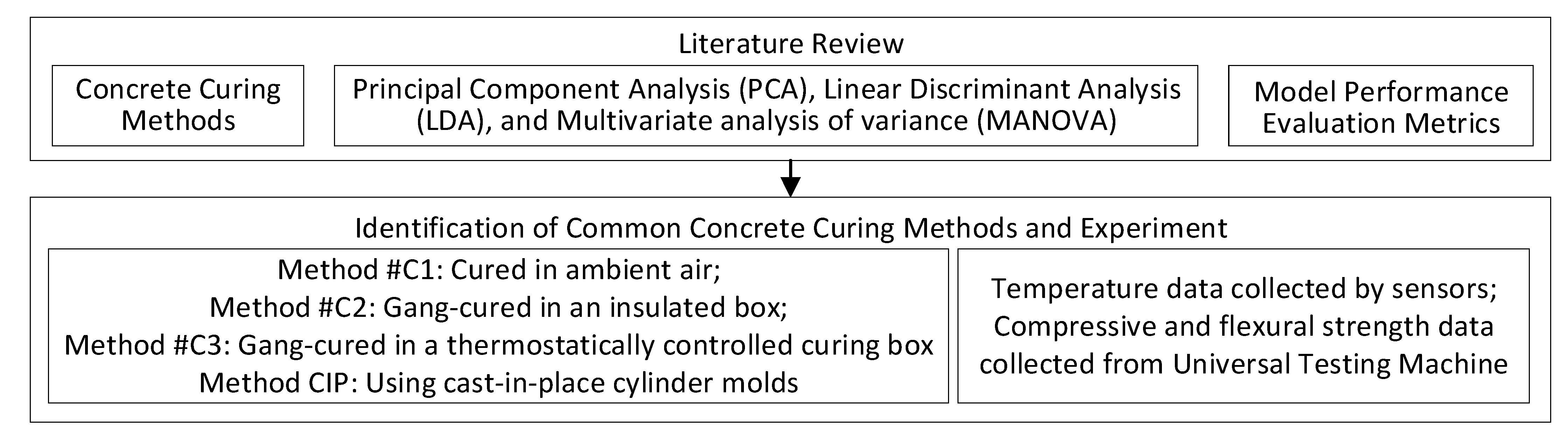
Figure 1 shows the theoretical framework of this research. To solve the research questions, we conducted a literature review that explored and identified the concrete curing methods #C1, #C2, #C3, and CIP (see Table 1). PCA, LDA, and MANOVA are used to analyze the multivariate regressions and variances in the influence factors of the estimation of in-place concrete strength. Common performance indicators (like a confidence interval, correlation value, r, R-squared value, root-mean-square error (RMSE), mean absolute error (MAE), and mean absolute percentage error (MAPE)) are calculated to evaluate the accuracy of the predictions of the models. The definitions and details of the indicators are explained in the Research Methodology section.

The PCA algorithm in this research takes datasets of points in a multiple-dimensional space, for example, values of multiple independent variables like curing days, specimen type, season, method, and temperature, as the input. The output is a set of principal components, which have special directions that capture the most important patterns and variances in the datasets in the dimensional space. The algorithm is based on a covariance matrix of eigenvalues, which indicate how much variance is captured by each eigenvector, while eigenvectors represent the directions of the variables in the dimensional space. One limitation of PCA is the assumption of correlations among features [10,11]. For example, if the curing days, specimen type, season, method, and temperature components are unrelated, PCA cannot determine the principal component. In this research, the components were identified based on the literature review and empirical data.

LDA takes a dataset of points in n-dimensional space as the input, with the output as a set of principal components, which are the directions in that n-dimensional space capturing the most important patterns and variances in the dataset. Different from PCA, which is an unsupervised technique that disregards class labels within the data, LDA is a supervised approach, operating under the assumptions of normally (Gaussian) distributed data and consistent covariance matrices across each class. For example, after calculating the eigenvalues and eigenvectors of the covariance matrix of the components, LDA sorts the eigenvalues in descending order and selects the top k principal components. One limitation of LDA is that regressions cannot be logistic [13]. This research uses hypothesis testing to verify the covariance regression types for LDA. Additionally, PCA was performed before LDA to avoid over-fitting and regularize the problem. After using PCA and LDA, there are still multiple components affecting the design and selection of concrete curing methods. In this case, a MANOVA is implemented to analyze multiple response variables simultaneously. One disadvantage of MANOVA is that the results can become difficult to interpret when there are multiple related dependent variables. Therefore, the research method design uses MANOVA after PCA and LDA so that it can have reduced components or dimensions.

3. Research Methodology

In regression analysis, homoscedasticity refers to the assumption that the variances of errors are constant across levels of an independent variable. If this assumption is violated, it is known as heteroscedasticity, which can affect the validity of a regression model. In this research, one assumption was the homoscedasticity of the variance of errors (or residuals), which is verified in the Discussion section using regression models and variance analyses, using scatterplots with residuals against dependent variables to check homoscedasticity.

An analysis was conducted on the compressive and flexural strengths of 420 samples: 210 from the Turner Lab, 86 from the box culvert project, and 28 from the wing wall project. Solanki and Xie [9] showed the details of data collection using sensors for the temperature and moisture of ambient air, specimens, curing boxes, and in situ concrete structure items, along with the concrete strengths using experiments and a universal testing machine. MATLAB (R2022a) software, Python 3.11.5, and Minitab Statistical (R21.3) software were used for data analysis. This research implemented a crossmatching method to create coordinate pairs and help understand the correlation between two variables [9]. Figure 2 shows the procedure for generating regression results for the linear correlation analysis of the compressive strengths of 4 in. cylinders and 6 in. cylinders cured using only Method #C1. The procedure was based on ordinary least squares (OLS), which is a linear regression analysis method used to minimize the sum of squares of the differences between the output (y values) of the target linear function of the independent variable and the values of the variable being observed in the input dataset (x values). The OLS method was selected for its simplicity, interpretability, and good fit to the data, as evidenced by the high R-squared value and low p-values for the coefficients (see Discussion).

Figure 3 shows an example of the result from the regression analysis (in Figure 2). There are 186 observations in the paired dataset. The calculation of degrees of freedom of residuals is to calculate the total number of observations (rows) subtracted by the number of variables being estimated using the dataset. In this case, the degree of freedom of residuals is 186 − 2 = 184. The degree of freedom of the model is 1.

The R-squared (R²) value is the coefficient of determination (see Equation (1)). The higher the value, the better the goodness of fit of a model. In Figure 3, the R-squared value is 0.975, which means that 97.50% of the variation in the y values is accounted for by the x values. The R-squared indicator measures the strength of the relationship between the prediction of a linear model and its dependent variable to show how well a regression model describes observed data. The main purpose of using an R-squared indicator is to avoid overfitting a model, meaning preventing the model from picking up noise. Nevertheless, the criteria value of R-squared depends on the context. In this research, the R-squared indicator is set to be 0.8 or higher [16].

$$R^2=1-\frac{sum squared regression \left(SSR\right)}{total sum of squares \left(SST\right)}=1-\frac{\sum {\left(y_i-\widehat{y_i}\right)}^2}{\sum {\left(y_i-\overline{y}\right)}^2},$$

(1)

where i is a variable, y_i is the observed data, $\overline{y}$ is the mean of the observed data, and $\widehat{y_i}$ is the regression estimate.

The Adjusted (Adj.) R-squared in Figure 3 is the modified version of the R-squared value for the number of predictors in the model. The higher the better. The F-statistic is calculated as (MSR/MSE) = Mean sum of squares regression/Mean sum of squares error. Using an F Statistics table (F-Alpha, n.d.), alpha = 0.05, denom. degree of freedom = 184, and numerator degrees of freedom = 1, the f(critical value) = 3.890. The f-statistics of 7152 is greater than the critical value of 3.890, which means that there is statistical evidence for rejecting H0: β1 = 0 (or the coefficient of x variable is zero). The null hypothesis that the value of all coefficients = 0 is rejected. Thus, the alternate hypothesis holds, which means that the coefficient related to the predictor variable (the compressive strengths of 4 in. cylinders) is non-zero.

The Prob(F-statistic) in Figure 3 is the overall significance of the regression model and assesses the significance level of the overall variables. It is used to test the null hypothesis that “all the regression coefficients are zero.” Hence, the Prob(F-statistics) value is close to zero, which indicates that the probability of the null hypothesis being true is approximately zero. This implies that the regression model is meaningful. The AIC and BIC in Figure 3 stand for Akaike’s Information Criterion and Bayesian Information Criterion. The AIC (see Equation (2)) is used for model selection and calculated as the difference between the number of parameters and the likelihood of the overall model (see the equation below). It shows how well a model fits the data. A lower AIC implies a better model. The BIC (see Equation (3)) is a variant of AIC where penalties are made more severe. However, both AIC and BIC are for model comparison. A single AIC or BIC value is meaningless without iteration or comparison. In addition to the R-squared, three more indicators are used to examine the performances of correlation equations, including RMSE (Equation (4)), MAE (Equation (5)), and MAPE (Equation (6)).

$$AIC=2k-2ln\left(\widehat{L}\right),$$

(2)

$$BIC=kln\left(n\right)-2ln\left(\widehat{L}\right),$$

(3)

$$RMSE=\sqrt{\frac{{{\displaystyle \sum }}_{i=1}^N{\left(y_i-\widehat{y_i}\right)}^2}{N}},$$

(4)

$$MAE=\frac{{{\displaystyle \sum }}_{i=1}^N\left|\widehat{y_i}-y_i\right|}{N},$$

(5)

$$MAPE=\frac{1}{N}{{\displaystyle \sum }}_{i=1}^N\frac{\left|\widehat{y_i}-y_i\right|}{y_i}$$

(6)

where k = the number of estimated parameters in the model, $\widehat{L}$ = the maximum value of the likelihood function for the model, n = the number of data points or observations.

4. Discussion

4.1. Principal Component Analysis (PCA) and Linear Discriminant Analysis (LDA)

Table 3. Principal component analysis.

Eigen Analysis of the Correlation Matrix
Eigenvalue	1.9976	1.3152	1.1975	1.0525	0.8313	0.5378	0.0680
Proportion	0.285	0.188	0.171	0.150	0.119	0.077	0.010
Cumulative	0.285	0.473	0.644	0.795	0.913	0.990	1.000
Eigenvectors
Variable	PC1	PC2	PC3	PC4	PC5	PC6	PC7
Curing days	0.030	−0.094	−0.406	−0.693	0.578	0.104	0.017
Specimen type	0.012	−0.712	−0.223	0.028	−0.342	0.570	−0.002
Casting date	−0.276	0.034	−0.658	−0.097	−0.475	−0.489	0.121
Method	0.060	−0.610	0.447	−0.276	−0.017	−0.585	0.082
Replicate	0.008	0.326	0.329	−0.655	−0.546	0.241	0.022
Max air temperature	0.670	0.013	−0.178	−0.032	−0.148	−0.157	−0.686
Min air temperature	0.685	0.067	−0.113	0.054	−0.058	−0.010	0.712

shows the PCA results of concrete curing methods based on the data features shown in the Table A1 in Appendix A. The compressive strengths of the cylinders and the flexural strengths of the beams are the dependent variables for the multivariate regression and variance analysis. The influence factors for concrete strengths are curing days, specimen type, casting date, method, replicate, max air temperature, and min air temperature. The negative value of a component in Table 3 means that the component is not significant. The first principal component accounts for 28.5% of the total variance. The variables that correlate the most with the first principal component (PC1) are min air temperature (0.685), max air temperature (0.670), method (0.060), and curing days (0.030). The first principal component is positively correlated with all the variables except the casting date. The first four principal components explain 79.5% of the variation in the data. Therefore, these components can be used to analyze concrete strength prediction. In this research, the method variable was used to classify observations.

Table 4. Squared distance between groups for LDA.

Group	1	2	3	4	6
1	0.000	0.748	2.639	309.292	1.788
2	0.748	0.000	1.375	319.115	1.192
3	2.639	1.375	0.000	314.887	0.192
4	309.292	319.115	314.887	0.000	314.409
6	1.788	1.192	0.192	314.409	0.000

lists the squared distance between groups. The more distinct the value is, the better the classification in the LDA.

4.2. Correlation Analysis: 4 in. vs. 6 in. Cylinders (Curing Method #C1)

Figure 4 shows the fitted line plots, and

Table 5. Explanations for the correlation analysis in Figure 4 (for the correlation analysis of the compressive strengths of 4 in. cylinders and 6 in. cylinders cured using Method#C1).

#	Explanation
(a)	The plot shows a linear correlation: y = 228.0869 + 0.9325x, R-squared = 0.9750.
(b)	Further analysis of the linear correlation of (6 in. compressive strength = coefficient × 4 in. compressive strength) for all curing days. The y-intercept is zero. Compared with the model equation in Figure 4a, this assumption fits engineering practice because right after the concrete is poured, it does not gain any compressive strength at time zero. The result model equation shown in Figure 4b is y = 0.9836x, for the data of compressive strengths tested during all curing days including Days 1, 2, 3, and 7. The corresponding R-squared is 0.9955, which indicates that the result model equation is accurate in describing the correlation of the observations.
(c)	Based on the PCA in Table 3, the variable curing days can affect the correlation between the compressive strengths of different cylinders. Hence, further analysis was performed after only one day of curing duration. The figure shows the result when setting the y-intercept to zero. The result model equation is y = 1.0497x. The R-squared value = 0.9889. The model equation is accurate in describing the correlation of the observations.
(d)	It shows further analysis of the linear correlation: (6 in. compressive strength = coefficient × 4 in. compressive strength) using summer data. The y-intercept is zero. The result model equation is y = 0.9603x. The R-squared value = 0.9910. The model prediction is accurate.
(e)	It is a further analysis of the linear correlation using fall data. The y-intercept is zero. The result model equation is y = 0.9947x. The R-squared value is 0.9958. The model equation is accurate.
(f)	result model equation is y = 0.9799x. The R-squared value is 0.9962. The results indicate that the model equation is accurate in describing the correlation of the observations.
(g)	The result model equation is y = 0.985x. The R-squared value is 0.9956. The results indicate that the model equation is accurate in describing the correlation of the observations.
(h)	It is the fitted line plot for the nonlinear correlation. See Table 6 for details.

has explanations about the plots. The plots are generated using the compressive strengths of 4 in. cylinders as the x-axis and the compressive strengths of 6 in. cylinders as the y-axis. The nonlinear analysis (Figure 4h) assumes three independent variables (x1, x2, and x3) and one dependent variable. In this case, the degree of freedom of residuals is 186 − 4 = 182. The degree of freedom of the model is 3. The R-squared value and the Adjusted R-squared value are 0.967, which means that 96.70% of the variation in the y values is accounted for by the x values. The f-statistic of 1799 is greater than the critical value of 2.6790, which means that the null hypothesis that the value of all coefficients = 0 is rejected. Thus, the alternate hypothesis holds, which means that the coefficient related to the predictor variable (the compressive strengths of 4 in. cylinders) is non-zero. The Prob(F-statistic) value is close to zero, which implies that the regression model is meaningful.

Figure 5 shows the residual analyses of concrete compressive strength prediction when 4 in. and 6 in. cylinders were cured using Method #C1. The normal probability plots in Figure 5a,e use the residuals as the x-axis and the probability percentages as the y-axis. The residual for each observation is calculated as the difference between a predicted value of y and observed values of y. It is used to assess whether or not a dataset is approximately normally distributed. The data points are plotted against a theoretical normal distribution (the red lines in Figure 5a,e). The points form an approximate linear pattern in Figure 5a,e, which indicates that a normal distribution can be used for this dataset.

Figure 5b,f shows residual versus fit plots resulting from residual analysis, where residuals are on the y-axis and fitted values (a.k.a., estimated responses) are on the x-axis; the analysis detects non-linearity, unequal error variances, and outliers. The residual = 0 line corresponds to an estimated correlation regression line (e.g., in Figure 4). The residuals in Figure 5b,f are distributed randomly around the corresponding zero lines. Additionally, the residuals roughly form a horizontal box shape around the zero lines in Figure 5b,f, which suggests that the variances of the error terms are equal. A few residuals are quite different from the basic random pattern of residuals, which suggests that there are outliers. Figure 5c,g shows the histograms of the residual frequency. The zero residuals have the most frequencies, and the negative and positive residuals are evenly distributed in these two figures. The histograms show normal distributions. Figure 5d,h shows the standardized residuals in the order of the corresponding observations. When the order of the observations may influence the results, data are collected in a time sequence or some other sequence, or from different geographic areas in a certain order. These plots can help to check whether designed experiments (in which the runs are performed) are randomized. The residuals in both plots fluctuate in a random pattern around the center line of zero. No correlation exists between error terms that are near each other. No ascending or descending trend in the residuals is shown in the correlation among residuals.

Table 6. Comparison of linear vs. nonlinear correlation models of the compressive strengths of 4 in. and 6 in. cylinders cured using Method #C1.

	Linear Model	Nonlinear Model	Modified Linear Model	Evaluation
Model equation	y = 228.0869 + 0.9325x	y = 1.14 × ${10}^{-9}+1.23\times {10}^{-6}\left(x_1\right)+0.001\left(x_2\right)$ $-4.63\times {10}^{-7}\left(x_3\right)+7.27\times {10}^{-11}\left(x_4\right)-4.03\times {10}^{-15}\left(x_5\right)$	y = 0.9836x	Better in simplicity and easiness of use
C.I.	95%	95%	95%	Same
Correlation type	Pearson’s	Pearson’s	Modified Pearson	--
Data points	186	186	186	Same
Correlations	0.9870	0.9870	0.987	Same
R	0.9870	0.9840	0.9847	A higher value is preferred
R-squared	0.9750	0.9670	0.9696	A higher value is preferred
RMSE	251.2410	286.5370	276.4787	A smaller value is preferred
MAE	196.9860	234.5930	216.3038	A smaller value is preferred
MAPE	0.065	0.1100	0.0734	A smaller value is preferred

summarizes the linear and nonlinear correlation analysis of the compressive strengths of 4 in. and 6 in. cylinders cured using Method #C1. The results indicate that the linear equation y = 0.9836x is reliable to describe the correlation and has a better performance.

4.3. Correlation Analysis: 4 in. vs. 6 in. Cylinders (Curing Method #C2)

There are 192 observations in the paired dataset for the correlation analysis of the compressive strengths of 4 in. cylinders and 6 in. cylinders cured using only Method #C2. The degrees of freedom of residuals is 192 − 2 = 190. The degree of freedom of the model is 1. The R-squared value is 0.913. The Adjusted R-squared value is 0.912 for the number of predictors in the model. The F-statistic of 1989 is greater than the critical value of 3.890, which means that the coefficient related to the predictor variable (the compressive strengths of 4 in. cylinders) is non-zero. The Prob(F-statistic) is close to zero, which implies that the regression model is meaningful. Figure 6 shows the fitted line plots when using the compressive strengths of 4 in. cylinders as the x-axis and the compressive strengths of 6 in. cylinders as the y-axis.

Figure 7 shows the residual analyses of the influences of Method #C2 when using the residuals as the x-axis and the probability percentages as the y-axis. Figure 7a,e shows the normal probability plots. The points in Figure 7a form an approximate linear pattern, which indicates that a normal distribution can be used for this dataset. The points in Figure 7e have outliers in the lower left corner. The residual versus fits plots in Figure 7b,f detect non-linearity, unequal error variances, and outliers. The residuals distribute randomly around the zero line, which suggests that the assumption that the relationship is linear is reasonable. Additionally, the residuals of (y_actual − y_predicted) are on the y-axis and have a wider span around the zero line above the 3500 psi fitted values of the estimated compressive strengths of the 6 in. cylinders than the ones in the range of 2000 psi to 3500 psi, which suggests that the variances of the error terms increase when the estimated compressive strengths of the 6 in. cylinders increase. Then, the variances stay the same after the 3500 psi value. A few residuals are different from the basic random pattern of residuals, which suggests that there are outliers.

Figure 7c shows the histogram of the residual frequency for the corresponding linear regression. The zero residuals have the most frequencies, and the negative and positive residuals are evenly distributed. The histogram has a normal distribution. In Figure 7g, the zero residuals have the most frequencies, and the positive residuals are more than the negative residuals; hence, the histogram is skewed. Figure 7d,h shows the standardized residuals in the order of the corresponding observations of the corresponding regressions. The residuals fluctuate in a random pattern around the center line of zero. No correlation exists between error terms that are near each other. No ascending or descending trend in the residuals is shown in the correlation among residuals.

Table 7. Explanations of the correlation analysis in Figure 7.

#	Explanation
(a)	Linear correlation: y = 1067.0 + 0.81x, R-squared = 0.9130.
(b)	When the intercept is set to zero, y = 1.0361x for the data of compressive strengths tested during all curing days including Days 1, 2, 3, and 7. R-squared = 0.9903.
(c)	Using Day 1 data and setting the y-intercept to zero. y = 1.1237x, R-squared value = 0.9889.
(d)	Using summer data and setting the y-intercept to zero. y = 0.9851x, R-squared value = 0.9959.
(e)	Using fall data and setting the y-intercept to zero. y = 1.0407x, R-squared value = 0.9910.
(f)	Using winter data and setting the y-intercept to zero. y = 1.1119x, R-squared value = 0.9861.
(g)	Using spring data and setting the y-intercept to zero. y = 1.0674x, R-squared value = 0.9925.
(h)	For the nonlinear correlation analysis, see Table 8 for details.

Note. The 4 in. cylinders and 6 in. cylinders are cured using only Method #C2.

compares the performances of the correlation and regression. The correlations were generated using the compressive strengths of the 4 in. cylinders as the x-axis and the compressive strengths of the 6 in. cylinders as the y-axis.

There are 192 observations in the paired dataset. The nonlinear analysis assumes three independent variables (x1, x2, and x3) and one dependent variable. In this case, the df of residuals is 192 − 3 − 1 = 188. The degree of freedom of the model is 3. The R-squared value and the Adjusted R-square value are 0.904 and 0.903, respectively, which means that 90.40% of the variation in the y values is accounted for by the x values. The F-statistic of 593.1 is greater than the critical value of 2.6790, which means that the alternate hypothesis holds, and the coefficient related to the predictor variable (the compressive strengths of the 4 in. cylinders) is non-zero. The Prob(F-statistic) value is close to zero, which implies that the regression model is meaningful.

Table 8. Comparison of linear vs. nonlinear correlation models of the compressive strengths of the 4 in. and 6 in. cylinders cured using Method #C2.

	Linear Model	Nonlinear Model	Modified Linear Model	Evaluation
Model equation	y = 1067.0 + 0.81x	y = 9.227 × 10−10 + 1.365 × 10−6(x1) + 0.0013(x2) −4.784 × 10−7(x3) + 6.891 × 10−11(x4) − 3.514 × 10−15(x5)	y = 1.0361x	The linear model is better in simplicity and easiness of use
C.I.	95%	95%	95%	Same
Correlation type	Spearman, Pearson’s	Spearman, Pearson’s	Modified Pearson’s correlation	--
Data points	192	192	192	Same
Correlation	0.955	0.955	0.955	Same
r	0.955	0.951	0.8762	A higher value is better
R-squared	0.913	0.904	0.7677	A higher value is better
RMSE	329.983	345.441	38.8653	A smaller value is better
MAE	260.41	273.818	421.8578	A smaller value is better
MAPE	0.062	0.073	0.0965	A smaller value is better

compares the model performances of the linear and nonlinear equations of the correlation models of the compressive strengths of the 4 in. and 6 in. cylinders cured using Method #C2. The results indicate that the linear model is better in performance. The modified Pearson’s correlation method in the table follows the Wilkinson–Rogers notation to describe regression in a simplified manner by making specific coefficient values into zeros. This modified Pearson’s correlation method identifies the response variable based on the previous linear and nonlinear correlation analyses.

Figure 8a shows the following fitted lines based on the results in Table 6. In general, the compressive strengths of the 4 in. cylinders show slightly higher values than the compressive strengths of the 6 in. cylinders cured using Method #C1.

• $y1=228.0869+0.9325x$, for experiments performed on Days 1, 2, 3, and 7.
• $y2=0.9836x$, for experiments performed on Days 1, 2, 3, and 7 starting from the origin point (0,0).
• $y3=1.0497x$, for estimated strength correlations 24 h (Day 1) after casting concrete cylinders.

Figure 8b shows the following fitted lines based on the results in Table 8. In general, the compressive strengths of the 4 in. cylinders show slightly lower values than the compressive strengths of the 6 in. cylinders cured using Method#C2.

• $y1=1067.0+0.81x$, for experiments performed on Days 1, 2, 3, and 7.
• $y2=1.1518x$, for experiments performed on Days 1, 2, 3, and 7 starting from the origin point (0,0).
• $y3=1.058x$, for estimated strength correlations 24 h (before Day 1) after casting concrete cylinders. The line then continues with a linear line of y5 = 0.8542x for the rest of the days.

4.4. MANOVA

Table 9. MANOVA.

MANOVA Tests for Specimen Type
			Degree of Freedom
Criterion	Test Statistic	F	Num	Denominator	p-Value
Wilks’	0.91681	3.856	2	85	0.025
Lawley–Hotelling	0.09074	3.856	2	85	0.025
Pillai’s	0.08319	3.856	2	85	0.025
Roy’s	0.09074
s = 1 m = 0 n = 41.5
MANOVA Tests for Method
Wilks’	0.29181	24.117	6	170	0
Lawley–Hotelling	2.05575	28.781	6	168	0
Pillai’s	0.81647	19.776	6	172	0
Roy’s	1.85579
s = 2 m = 0 n = 41.5
MANOVA Tests for Season
Wilks’	0.06122	86.179	6	170	0
Lawley–Hotelling	10.79215	151.09	6	168	0
Pillai’s	1.21687	44.544	6	172	0
Roy’s	10.3534
s = 2 m = 0 n = 41.5
MANOVA Tests for Specimen Type × Method
Wilks’	0.91727	1.25	6	170	0.283
Lawley–Hotelling	0.08935	1.251	6	168	0.283
Pillai’s	0.0835	1.249	6	172	0.284
Roy’s	0.0787
s = 2 m = 0 n = 41.5

assesses the compressive strengths and flexural strengths of the specimens (4 in. cylinders, 6 in. cylinders, and 20 in. beams). The specimens were cast and cured using different methods listed in Table 1 and tested after 1, 2, 3, and 7 days. The MANOVA was used to determine whether the curing method, specimen types or sizes, curing duration, and season of construction affect concrete strengths. The degree of freedom denominator is used to calculate F. The s, m, and n values are degrees of freedom. The p-values are set at the 0.10 significance level for any of the tests. The p-values for specimen type (0.025 < 0.10), method (0 < 0.10), and season (0 < 0.10) are statistically significant at the 0.10 significance level. The p-values for the interaction between specimen type and method (0.283 > 0.10) are statistically insignificant at the 0.10 significance level. Because the interaction is statistically insignificant, the effect of the method depends on the season.

4.5. Outcomes Analysis

The investigation shows that min air temperature, max air temperature, curing method, and curing days are the principal components of concrete construction (see Table 3). A further linear discriminant analysis (LDA) shows that the curing method variable should be used to classify observations (see Table 4). For all the concrete specimens cured using Method #C1, the linear correlation regression equations in Table 5 have R-squared values of (a) 0.9750, (b) 0.9955, (c) 0.9889, (d) 0.9910, (e) 0.9958, (f) 0.9962, and (g) 0.9956, and the nonlinear correlation regression equation in Table 6 has an R-squared value of 0.9670. All the R-squared values are greater than 80%, which confirms the applicability of Gaussian process regression (GPR). The predictions of GPR for a new data point are based on the conditional distribution of the corresponding variable given observed data. Hence, GPR is applicable for the outcome analysis because, for a given set of function values, their combined distribution follows a pattern (a.k.a., multivariate Gaussian). This pattern and its specific details, like averages and variances, are already determined with prior knowledge.

Similarly, for all the concrete specimens cured using Method #C2, the linear correlation regression equations in Table 7 have R-squared values of (a) 0.9130, (b) 0.9903, (c) 0.9889, (d) 0.9959, (e) 0.9910, (f) 0.9861, and (g) 0.9925, and the nonlinear correlation regression equation in Table 8 has an R-squared value of 0.9049. All the R-squared values are greater than 80%, which confirms the applicability of GPR.

Further examination indicates that the multiple linear regression (MLR) model in Table 5 has different slopes in the correlation regression equations of the compressive strengths of the 4 in. and 6 in. cylinders when using Method #C1 to cure them. The slopes are in the range of [0.9603, 1.0497], with a 9.31% difference. Using the 24 MPa (3500 psi) design standard as an example, the difference is 24 × 9.31% = 2.23 MPa (or 325 psi). The slope differences suggest that concrete construction in different seasons could have a nearly 2.24 MPa variation in compressive strength estimation when using 4 in. or 6 in. cylinders. Table 7 has the same influence factors as Table 5, except that the data are for Method #C2. The slopes are in the range of [0.9851, 1.1237], with a 14.07% difference, which suggests that the MLR model should consider construction season and curing duration.

The real-world data collected using sensors and experiments in this paper was verified by multiple transportation construction experts and engineers. Compared with the studies of [17,18], the data and the findings help establish baselines, find benchmarks, and set performance goals for concrete construction. Furthermore, the observations on the results of Table 5 and Table 7 reveal that for the early strength development of concrete, the slopes of the correlation regression equations for both Method #C1 (y = 1.0497x) and Method #C2 (y = 1.0361x) are greater than 1, which implies that the 6 in. cylinders overestimate the compressive strengths of in-place concrete compared with the 4 in. cylinders. One reason is that more heat is generated from 6 in. cylinders than 4 in. cylinders during cement hydration reaction.

One practical implication of the findings for construction professionals is that they should be aware that the specimen size difference can lead to the risk of loading stress on a concrete structure before it matures. This research used the test data for the curing durations of 1–7 days, which indicate concrete early strengths. When using 6 in. cylinders for concrete strength testing, construction professionals can reduce the test results of compressive strengths by 9% when using an ambient air curing method and 14% when using an insulated box curing method for concrete early strengths of 1 to 7 days. The analysis shows that the quality control of concrete construction projects relies on the data-driven decision-making of curing method selection. For example, this research used 3500 psi as the target compressive strength of the concrete mixture design. The compressive strength can be 7000 psi for precast and prestressed concrete and 15,000 psi for load-bearing columns. Hence, the decisions on curing methods and cylinder types have increased influences on the accuracy of the strength estimation of high- and ultra-high-strength concrete. Particularly, these decisions need to be made before the start of construction. In this case, construction professionals and engineers should be cautious when using 6 in. testing cylinders for high-early strength concrete or precast and prestressed concrete.

Moreover, this recommended practice can help the concrete industry reduce the potential risks of applying loads to premature concrete structures. Possible consequences of over-estimating in-place concrete strength in construction projects include structure failure, reduced durability, and possible concrete cracking. Usually, the practical application of avoiding over-estimation is to multiply a safety factor or empirical value. This research improved the accuracy and reliability of concrete compressive strength estimates, which can help concrete quality control and resource allocation.

5. Conclusions

The design and selection of a concrete curing method are critical to quality control and project success. This research emphasizes that the process of maintaining the moisture and temperature conditions in concrete is necessary for cement hydration, and the curing result of in-place concrete is ensured by testing specimens to verify that the concrete develops its desired strength and durability. Furthermore, this paper presents an innovative multivariate regression analysis for the correlation and variance of different temperatures of construction seasons, duration of curing days, specimen sizes, and curing methods.

The seven most common curing methods were investigated based on the identified influencing factors of concrete strength. The findings of this paper shed light on the establishment of variance analysis methods in the context of concrete construction with commonly used multivariate regression models. The findings can also support decision-making for specimen sizes and concrete curing methods. Another practical implication of this paper is to improve confidence when construction professionals estimate in-place concrete strength.

Test concrete is important to ensure that it has achieved its desired strength and durability [18]. The duration of the curing process varies depending on the concrete type, admixture, and environmental conditions. This paper provides a systematic comparison between prediction results and experiment outcomes and a discussion of how various influencing factors cause an overestimation of in-place concrete strength. The comparison between prediction results and experiment outcomes indicates that during the early strength development period of concrete (1 to 7 days), the compressive strengths of 6 in. testing cylinders are approximately 9% higher than 4 in. cylinders when using an ambient air curing method and 14% higher when using an insulated box curing method. The discrepancies are derived using PCA, LDA, MANOVA, and correlation regression methods and have R-squared values over 90%, which indicates the accuracy and reliability of the analysis. This research helps to improve the reliability of concrete strength prediction. For example, using the MLR and MANOVA models, if the concrete (like high-early strength concrete) specimen testing after Day 1 shows satisfactory results, engineers can confidently open the construction for the project. Or they can arrange a strength test of specimens after the second day of casting concrete instead of waiting for three days or seven days. This can reduce the usage of a considerable amount of financial resources and shorten waiting or idling time.