Abstract
A new technique for two-dimensional vortex methods is presented. The vorticity field is discretized and represented by vortex blobs. Viscosity and roughness are incorporated into vortex simulations by means of the corrected core-spreading method with LES theory. A deterministic and efficient grid-free method simulates viscous effects by maintaining small vortex core sizes through a splitting algorithm that controls the consistency error. The LES theory also enables the implementation of the roughness model. The effectiveness of this method is shown in calculating vortex interactions and decay in aircraft wakes with crosswind near a rough ground plane. The numerical results of the trajectory of primary vortical structures are compared with experimental data (when possible), suggesting the validity of the method. In general, the control of the roughness height size appears as an important factor to interfere on the trajectory of primary vortical structures in the ground effect with crosswind. The effect of the relative roughness height of ε/Δs = 0.001 shows that the primary vortical structures survive the interaction with the ground plane and can attain a maximum height in the order of 0.95 h (h is the release height of the primary vortical structures) during the loop for crosswind velocity of U∞ = 0.02 at Re = 7650. On the other hand, the combined effects of roughness ε/Δs = 0.001 and of crosswind U∞ = 0.04 at Re = 75,000 indicate that the primary vortical structures attain a maximum height about 0.83 h during the loop, tending to leave the runway faster, with sufficient intensity to disturb a smaller aircraft operating on a parallel runway.
1. Introduction
Turbulence is a very frequent phenomenon in almost all engineering flows. For flows with a low Reynolds number, the viscous part (dissipative) strongly acts to stabilize such flows. However, an increase in Reynolds number disorganizes the flows, making them turbulent [1]. As an example of the complexity of turbulent phenomena, Ozkan and Egitmen [2] examined the substantial changes in turbulent flow structures and flow characteristics around a NACA 0012 airfoil using two-dimensional PIV measurements and concluded that the vortical interactions and consequent fluctuations in the near wake of airfoil were gradually intensified with an increasing Reynolds number for zero angle of attack (λ = 0°), whereas the reverse was the case for λ = 5°. So, the crucial issue presented to the scientific community is to solve the flows when they are turbulent, and with such purpose, new models are frequently proposed in the literature [3].
The Navier–Stokes equations have existed since 1822, and it is necessary to handle different flow scales to solve the equations. In other words, it is mandatory to understand the vortical structure behavior for all frequencies and scale lengths. Nowadays, it is still impractical to solve the Navier–Stokes equations with that prism. The turbulence has been additionally studied for more than eight decades, and there is no easy/general solution to solve turbulent flows; as a consequence, lots of turbulence models have been developed by researchers in different study centers around the world [4].
A spectrum with all frequencies and scale lengths of the vortical structures into the flow field is available in large-eddy simulation (LES). The large scales can be directly solved in a typical direct numerical simulation (DNS), and the sub-grid scales must be modeled using a turbulence model. The use of LES theory blended with the second-order velocity structure function model is a tool that enables the development of Lagrangian vortex methods with roughness models. In this context, our research group reported in the literature that a two-dimensional surface roughness model is more sensitive to capture nonlinear hydrodynamic phenomena than a simple turbulence model [5,6,7,8]. That research line is effective and produces interesting numerical results to be applicable in engineering conservative designs.
Lagrangian vortex methods are a very interesting alternative to simulate unsteady and vortical flows because the technique provides a direct simulation of the real vortical structures in the most economical manner, being applicable to a wide range of industry problems [9,10]. The vorticity created at solid boundaries is discretized and represented by computation points (vortex elements or vortex blobs), which are strategically positioned only where there is vorticity in the fluid domain. The cluster of vortex blobs must be submitted to the advection and diffusion mechanisms. Also, the Lagrangian description for the vorticity field does not require the use of mesh, and the boundary conditions far from the solid boundaries are automatically satisfied.
The real history of the “Vortex Methods” began with the modelling of inviscid potential flows as presented by Martensen [11]. Chorin [12] and Leonard [13] contributed to the modern vortex method in terms of a time-stepping scheme to compute viscous effects and inviscid parts of the governing equations as successive sub-steps. Chorin [12] introduced the idea of the “fractional step” method or “viscous splitting” (a particular case of the general approach of “operator splitting”) blended with the random walk diffusion scheme, the latter a Brownian-like motion of the vortex blobs. Leonard [13] introduced the core-spreading algorithm (CSA) in a purely Lagrangian manner to take into account viscous effects by changing the core size of the vortex blobs to exactly solve the diffusion equation. Historically, Greengard [14] argued that the CSA was physically wrong and that it did not in fact converge to a system of equations originating from the Navier–Stokes equations. It was postulated that the vorticity field is correctly diffused; however, the vorticity advection is incorrectly computed, even in the limit of infinitely many vortices. Later, Rossi [15] proposed a solution for the CSA based on vortex blob splitting, which proved to be convergent and effective. The title “corrected core-spreading method” originated from the correction suggested for the CSA by Rossi [15]; however, no attempt to include turbulence modelling was incorporated by him.
As well as many Eulerian methods, which require the use of sufficiently refined meshes, Lagrangian vortex methods need a great number of vortex blobs to handle higher-resolution turbulent vortical structures, which rapidly increases the computational time cost. In order to overcome that crucial point, several algorithms have been developed over the years to reduce the computational time cost associated with vortex methods; most of them are based on multipole expansions [16,17], and the more recent algorithms use parallel implementation with CUDA technologies [18]. The vortex method has been also applied to build a neural network description of Lagrangian vortices and their interaction dynamics, aiming to reconstruct the high-resolution Eulerian flow field in a physically precise manner [19].
In this scenario, our research group has examined a spatial averaging model of turbulence in high-Reynolds-number flows for Lagrangian large-eddy simulation, including a roughness model [7,8]. The numerical approach incorporated viscous effects through the random walk diffusion scheme proposed by Chorin [12] blended with LES theory [5] and the rough wall model [7].
The present paper contributes to a new Lagrangian vortex method based on a scheme that combines a blob splitting algorithm [15] with LES theory [5] and a roughness model [7]. The second-order velocity structure function model of the filtered field is then used to compute the local kinetic energy spectrum [20]. The corrected core-spreading method with turbulence modelling is necessary to control the consistency error of the CSA, maintaining the maximum blob radius below a stipulated value. The roughness model is inspired by the key idea to include a new momentum source term because of additional inertial effects; the numerical strategy simulates the momentum injection into the boundary layer, which is effectively reflected, changing both the viscous core and the strength of the nascent vortex blobs [7].
The new algorithm is then applied to analyze the dynamic interactions of aircraft wake vortices in the vicinity of a rough ground plane at two Reynolds number values, namely Re = 7650 and 75,000. The combined effects of crosswind and roughness are investigated and compared with the configuration of a smooth ground plane. Comparisons with experimental data published by Liu and Srnsky [21] using Re = 7650 are also presented. The available experimental data are scarce and did not include combined effects of surface roughness and crosswind, which motivated the present paper to contribute to the literature.
The problem of the dissipation of aircraft vortex wakes has been the focus of extensive studies aiming to predict the potential hazard of wake vortices and their lifetime in the ground effect [22,23,24,25,26]. The air always flows from a region of high pressure to a region of low pressure, and in the case of the aircraft wing, air flows from below the wing to the upper surface of the wing. Physically, the air rotates as a consequence of trailing vortices created by a wing because of pressure differences, producing the lift of the wing. The literature classifies the circular motion that the air takes as a “vortex”. The term “wingtip vortex” relates to the vortex being generated at the wingtip. The vortices that increase in diameter and decrease in intensity as the time passes are called “trailing vortices” [25,26]. These extend for a reasonable distance behind the aircraft wing. The contrails observed when an aircraft flies high at cruising altitude, developing velocity of about 850 km/h, are from the engine, not the vortices. Contrails from wingtip vortices are usually seen when an aircraft flies at low speeds (e.g., 240 km/h) and low altitudes (e.g., 70 m) in humid ambient conditions. The most common situation to visualize contrails occurs at the ends of the aircraft flaps when they are extended for an aircraft approaching or leaving a runway. So, wingtip vortices are more intense for a configuration of an aircraft: heavy, slow, and flying in a clean configuration. However, the real interest is in investigating the potential hazard for an aircraft approaching on the same (or a parallel) runway, since vortex size is affected by proximity to the ground too. The effect of strong crosswinds is also a factor that can interfere with vortices; the intensity of a vortex is not directly affected by crosswinds but they contribute to the dissipation of trailing vortices faster than still air [27,28].
Recently, intending to avoid accidents, Holzäpfel et al. [27] assessed various aspects of developing pairwise wake vortex separations for approach and landing at Vienna airport using what the authors called the Wake Vortex Prediction System (WSVS). The simulation study evaluated the probability that wake vortices remain within a defined radius around the follower aircraft when separations are applied. This probability was compared to data collected at five international airports. It was found that for WSVS predictions, wake vortices in ground proximity resided within a distance of 25 m to the follower aircraft in 0.25% of the landings.
It is known that wake decay can be improved by introducing artificial perturbations. Xu et al. [28] used a large-eddy simulation to investigate air blowing and suction as active flow control methods on wake vortex decay. Thus, blowing and suction zones were embedded in the ground to generate airflow below the wake vortex tubes. According to the authors, it was found that even with a small blowing velocity, the aircraft wake strength could be reduced.
In further work, Xu et al. [29] used a large-eddy simulation to show that under certain conditions of crosswind, the wake vortex deformed sinusoidally and linked with its mirror counterpart, which may cause an imminent risk of the vortex corridor to aircraft landing or taking off on the same or parallel runway.
In a recent paper from our research group, Moraes et al. [30] utilized a Lagrangian temperature particle method to study buoyance effects on aircraft wake vortices near a ground plane; however, turbulence modelling and roughness effects were not included.
Talking about this field of application, the present paper contributes with a new method to investigate the combined effects of surface roughness and crosswind for the problem of vortex rebound followed by continued separation at approximately constant distance from the ground plane. The new technique discretizes the vorticity field using vortex elements. The method of images is chosen to precisely represent the ground plane. The corrected core-spreading method simulates the vorticity diffusion by maintaining vortex elements with small sizes through a deterministic approach using a splitting algorithm. The vorticity diffusion incorporates viscosity effects and includes the local eddy viscosity coefficient computation. The local eddy viscosity coefficient is computed for every vortex element during every time step of a typical numerical simulation. The roughness model is also supported by the local eddy viscosity coefficient computation. The second-order velocity structure function model is adopted to compute the eddy viscosity coefficient. More details of the new technique will be properly discussed in Section 3.
Finally, the surface roughness effects from a ground plane can contribute to important aspects of traffic control related to aerodynamic forces, the safe separation distance between flights in the vicinity of an airport, and wake vortex dissipation with buoyancy forces. Inevitably, strong vortical structures interact with the ground plane, and accidents can occur in subsequent operations, particularly in the 30~70 m range above ground level [26]. The objective of the present work is to investigate the surface roughness effects on wake vortices generated by a large aircraft, which is approaching or leaving a ground plane with crosswind.
2. Problem Description
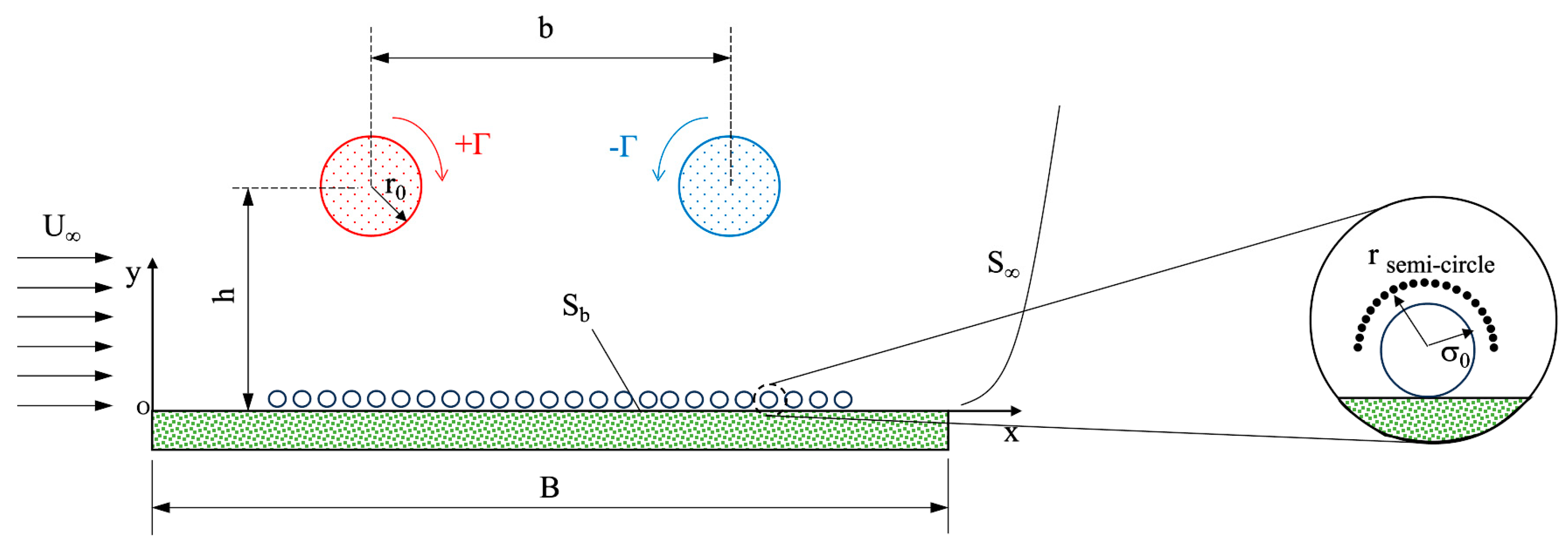
Figure 1 sketches the computational fluid domain (Ω) used in Lagrangian vortex method simulations, which contains a pair of vortical structures shedding from wingtips and rotating in opposite directions. The fluid domain is delimited by the ground plane surface, Sb, and the surface S∞ far from the wall plane, such that S = Sb ∪ S∞. The boundary conditions for the mathematical formulation must be imposed on S. The circulation strength is defined by Γ* = ±W*/(ρb*Ua*), where W* is the aircraft weight, ρ is the fluid density, b* is the wingspan, and Ua* is the aircraft approaching velocity. Here, all dimensional quantities are identified through the symbol *.

Figure 1.
Dimensionless computational domain.
In Figure 1, the inertial frame origin is located at x* = 0.0 and y* = 0.0. The ground plane length is defined by B*, and the starting positions of the center of the counter-rotating vortical structures are given by the coordinates x* = B*/2 ± b*/2 and y* = h*/b*. The crosswind is represented by the velocity U*∞. In general, relations around h*/b* = 2.0 are typical for the study of the potential hazard to aircraft when landing or taking off between parallel runways; in that situation, large aircraft usually develop velocity of approximately Ua* = 240 km/h [21].
All quantities are nondimensionalized by adopting the length scale b*, the representative velocity Γ*/b*, and the time scale b*/U*∞ (with crosswind) or b*2/Γ* (with no crosswind).
Every primary vortical structure shedding from the wingtip is discretized and represented by N Lamb discrete vortices or vortex blobs [31] randomly created there; the strength of one vortex blob is defined by Γ*/N. Vorticity is also instantaneously generated from the ground plane. Therefore, it must be represented by M nascent vortex blobs during every time-step, Δt, so as to satisfy the non-slip condition in specific points (or “pivotal points”) on the solid surface, Sb (Figure 1). On the other hand, the method of images [32] guarantees the impermeability condition at all points on the ground plane surface. A vortex blob is completely defined in two dimensions by position vector, vortex strength, Γv, viscous core, σ0, and vector velocity [31]. In a Lagrangian manner, every vortex blob must be individually followed during a typical numerical simulation.
The ground plane is divided into M flat panels of the same length, namely Δs*, with each equipped with a centered point, the so-called “pivotal point”. The dimensionless number ε/Δs (ε is the physical roughness height of the ground plane) is used to capture surface roughness effects of the ground plane in the simulation. Based on the typical roughness distribution of the ground plane, different roughness values can be chosen to be combined with different crosswind velocities, as will be discussed in Section 4.
3. Theory and Numerical Method
3.1. Governing Equations
In Figure 1, the flow because of the pair of primary vortical structures shedding from wingtips induces velocity on the solid surface, Sb. The effect of crosswind velocity can still be present in the fluid domain (Ω) to induce velocity on the ground plane too. Consequently, vorticity is continuously created from the ground plane and, once created, is free to undergo advection under all surrounding influences and diffusion under the action of viscosity. The governing equation for a two-dimensional, incompressible, and unsteady flow is given in terms of the vorticity transport equation of the filtered field [7]:
where is the fluid vorticity (the vorticity is a scalar in two dimensions), is the velocity vector, Re is the Reynolds number, and νt is the local eddy viscosity coefficient.
The Reynolds number is defined as in [21]:
where ρ is the fluid density, U∞ is the crosswind velocity, b* is the wingspan, μ is the dynamic viscosity, Γ* is the circulation strength, and ν is the kinematic viscosity (momentum diffusivity).
The turbulence manifestations are computed through the concept of the local eddy viscosity coefficient (instantaneously computed for every vortex blob), defined as follows [7,20]:
where Ck = 1.4 is the Kolmogorov constant, σ0 is the Lamb vortex core, and is the local second-order velocity structure function of the filtered field [5,20], namely:
In Equation (4), the summation must be computed by counting the number N of vortex blobs placed inside of an annulus, in which establishes the distance among the center of the annulus (center of the i-th vortex core under analysis) and centers of other vortex blobs located between the internal and the external radius of the same annulus [5,7] (e.g., k-th vortex blob is placed inside it).
Therefore, the large scales are solved through Equation (1) applied to the cluster of vortex blobs, and the sub-grid scales are modeled from Equation (4) using the concept of the local second-order velocity structure function of the filtered field. The surface roughness model adopted in this work is based on the fundamentals of turbulence modelling, as will be discussed in the next subsection.
3.2. Numerical Method
Chorin [12] proposed the “viscous splitting algorithm” for the Navier–Stokes equations that consists of sub-time-steps to successively compute the effects of advection and diffusion. Equation (1) is the well-known version of the Navier–Stokes equations with no pressure term. It is obtained by starting with the definition of vorticity () and applying the curl operator on Navier–Stokes equations (still assisted by the continuity equation). The Lagrangian version of Equation (1) is written as:
The vorticity advection problem is then governed by [12]:
and the viscosity is incorporated into vortex simulations as follows:
The vorticity created by the slip flow at the ground plane is then shed freely into the fluid. Figure 2a exemplifies the instantaneous creation and shedding of the second vortex blob along the ground plane. It is important to emphasize that M vortex blobs are shedding at every time-stepping of a typical numerical simulation. The centre of every nascent vortex blob (viscous core) is exactly located at the “shedding point”.
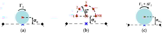
Figure 2.
Example of instantaneous shedding of a vortex blob from the second flat panel: (a) with no roughness model; (b) momentum injection model; and (c) with roughness model.
Figure 2b illustrates the key idea of the model to inject momentum during vorticity shedding from a flat panel. The practical effect is obtained in three steps, whose purpose is to change the viscous core, σ0, and the vortex strength, Γv, of every nascent vortex blob. Firstly, the vortex strength is obtained by solving a linear system of algebraic equations to ensure the non-slip condition on every “pivotal point”. The global circulation conservation (Kelvin’s theorem [33]) must also be satisfied. Secondly, a semicircle of radius , centered on a “shedding point”, is required to capture turbulent activities nearest a ground plane, where ε ≡ ε/Δs simulates the interference of a selected relative roughness height [7]. Bimbato et al. [7] adapted Equation (4), aiming to capture the velocity differences among the center of the i-th “shedding point” and NR = 21 “rough points”, as shown in Figure 2b (see also in Figure 1), where:
and (1 + ε) represents the kinetic energy gain because of surface roughness effects. Bimbato et al. [8] concluded that a set of NR = 21 “rough points” on each semicircle is sufficient to compute the average velocity differences necessary to evaluate the second-order velocity structure function of the filtered field, .
Thus, in response to Equation (8), the viscous core must be corrected accordingly to yield [7]:
Thirdly, the vortex strength is also corrected by again solving the linear system of algebraic equations to ensure the non-slip condition on every “pivotal point”. Figure 2c illustrates the effective creation and shedding of the second vortex blob with the surface roughness model. The roughness model can be physically interpreted as a new momentum source term for the Navier–Stokes equations because of additional inertial effects nearest the rough ground plane. The advective velocity components of i-th vortex blob are computed taking into consideration the contributions of crosswind velocity (when included), the cluster of vortex blobs (the Biot–Savart law), and their images (method of images) placed below the ground plane (Figure 1). The Biot–Savart law is evaluated through [9]:
where n represents two velocity components, NV is the total number of vortex blobs, is the strength of every vortex blob, and represents the nth component of the velocity induced by the j-th vortex blob (of unitary strength) at location of the k-th vortex blob. It is important to observe that vortex images only induce velocity.
Equation (6) indicates that vorticity is conserved during advection solution [34]. Thus, the advection problem is numerically solved by interpreting every vortex blob as a fluid material particle, whose trajectory equation is computed by an explicit Euler scheme [35], such as:
Equation (7) is numerically solved based on the vortex blob splitting algorithm proposed by Rossi [15]. The corrected core-spreading method avoids the consistency error of the core-spreading algorithm (CSA) caused by advection, not including the deformation of larger and larger vortex blobs as they spread.
The contribution of this paper is then to simulate Lagrangian vortices interactions using a large-eddy simulation (LES) and surface roughness model blended with the CSA corrected by Rossi [15].
Thus, the diffusion part in Equation (5), which is separated in Equation (7), is solved at every time-step, Δt, in agreement with:
where is i-th viscous core.
The originality of the present technique is to include the local eddy viscosity coefficient computation in Equation (12). The use of the second-order velocity structure function of the filtered field is advantageous over the Smagorinsky model when using a Lagrangian vortex method, since the concept of velocity fluctuations is used instead of the rate of deformation, see Equation (4). The velocity field computation is available to calculate the local eddy viscosity coefficient during every time increment of a typical numerical simulation.
As explained by Rossi [15], the core radius must be submitted to the partition scheme when it reaches the maximum permissible/controlled value. That numerical strategy creates four new vortex blobs (starting from the original vortex blob), each with a quarter of the original circulation and a core radius given by . Then, the vortex blobs must be positioned at 90°, and every other is at a distance r given by:
where that distance is measured from the center of the vortex blob before suffering partition, and the partition scheme is governed by parameter α [0, 1]. It is clear that the maximum permissible value for the core radius is not a determining factor for the convergence of the method, unlike α.
A typical algorithm of Lagrangian vortex method simulation to take account of all these effects is implemented using an in-house code via parallel computing (OpenMP); it can be summarized as follows:
- (i)
- Initial specifications of geometry including M “shedding points” (every one above the “pivotal points”) and starting flow.
- (ii)
- Construction of the pair of counter-rotating vortical structures shedding from wingtips.
- (iii)
- Creation and shedding of M vortex blobs with no roughness model to ensure the no-slip condition on all “pivotal points” including global circulation conservation.
- (iv)
- Correction for viscous core and vortex strength of all nascent vortex blobs because of surface roughness effects.
- (v)
- Computation of the velocity field at every vortex blob location in the real plan (y > 0), as sketched in Figure 1.
- (vi)
- Advection of the cluster of vortex blobs.
- (vii)
- Computation of turbulence manifestations at every vortex blob location.
- (viii)
- Vorticity diffusion using the corrected core-spreading method with LES theory.
- (ix)
- Reflection of vortex blob that accidentally migrates into the ground plane.
- (x)
- Computation of the velocity field at every “pivotal point” to ensure the no-slip condition and, consequently, to obtain a new generation of vortex blobs.
- (xi)
- Advance time by Δt.
4. Results and Discussion
In this section, the focus is to discuss the numerical results and their contributions to produce a better understanding of the investigated physics. Firstly, Section 4.1 presents the convergence of Equation (11) applied for the advection problem of a pair of vortex blobs of equal strength Γv; a simple motion is simulated, in which time elapses over a succession of elementary but finite steps Δt. The convergence of the diffusion problem is presented through the application of Equation (12) to solve the diffusion of a vortex sheet.
Secondly, Section 4.2 investigates the trajectory of the centroid of the primary vortical structure from the right, as sketched in Figure 1. The trajectories are influenced by interaction with secondary vortical structures generated from the ground plane.
The sensitivity of the new technique is captured, and the results are interpreted by varying the Reynolds number value (i.e., Re = 7650 and 75,000), the relative roughness height (i.e., ε/Δs = 0.0, 0.001 and 0.007), and the crosswind velocity (i.e., U∞ = 0.0, 0.02 and 0.04).
4.1. Advection and Diffusion Convergence
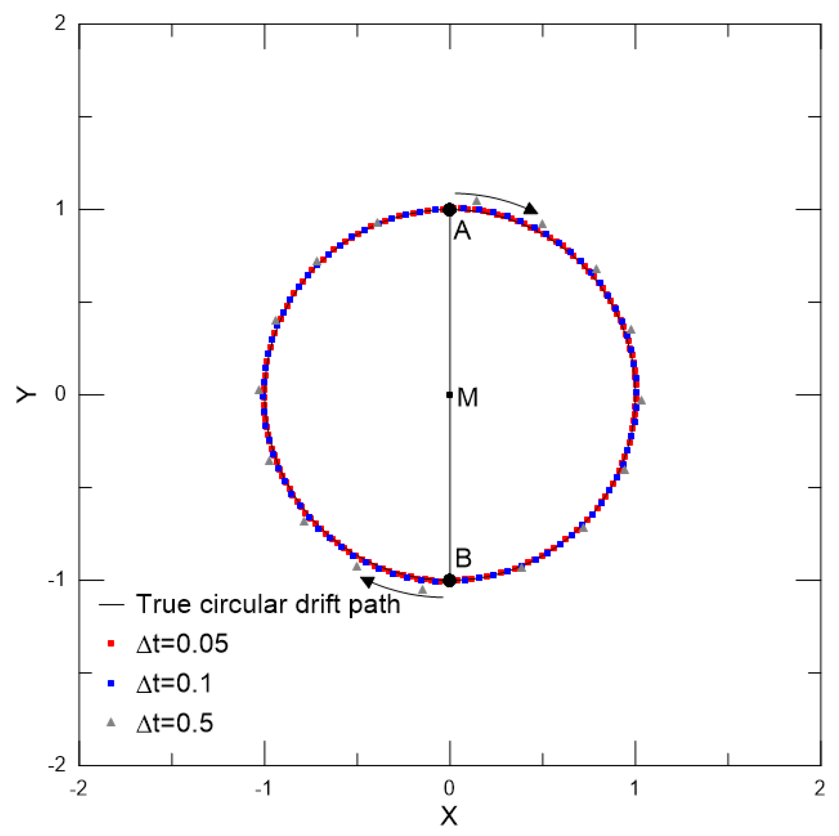
The convergence of Equation (11) is demonstrated through the problem of advection of a pair of vortex blobs. Figure 3 shows a vortex pair of equal strength Γv = 1, core radius σ0 = 0.001, distance AB = 2.0 apart. If these are free vortex, then they will induce velocity on each other (see Equation (10)), acting in the direction normal to the segment AB that joins them. Since there is no other contribution for the velocity computation, the vortex pair will process in a circular path (only advection motion) about the middle point of the line AB. Here, the adopted strategy is to stop the numerical simulation when the vortex blob A, starting at its original position (0.0, 1.0), approximately attains the starting position of the vortex blob B at location (0.0, −1.0).

Figure 3.
Convergence of the advection scheme using a pair of vortex blobs.
The relative error between the true circular drift path maintaining constant distance AB = 2.0 and the numerical result obtained by Equation (11) is about 4.27%, 0.88%, and 0.44% when time increments of 0.5, 0.1, and 0.05 are adopted, respectively. Thus, the time-stepping Δt = 0.05 is considered suitable to be used in the explicit Euler time marching scheme. Curiously, 795 time steps of magnitude Δt = 0.05 were required to satisfy the numerical simulation stopping criterion. An advantage of the Lagrangian manner over Eulerian schemes to compute vorticity advection is that no explicit treatment of advective derivatives is required.
The convergence of Equation (12) is noticed by comparing it with the analytical solution of the viscous diffusion of the finite length of a vortex sheet, say, between 0 < x < ℓ (ℓ is adopted equal to 0.3). That vortex sheet length can also be thought of as part of the ground plane length, i.e., the surface Sb in Figure 1. As shown by Batchelor [36], the analytical solution is given by:
where γ(x) = 2U represents the sheet strength, U = 1 defines the mainstream velocity, and 4t/Re is interpreted as vorticity penetration depth during the time t.
The adopted values to solve Equation (12) are M = 30 vortex blobs, every intensity Γv = γ(x) ℓ/M and generated on “pivotal points” on y = 0; core radius σ0 = 0.01; time corresponding to t = Δt = 0.22; Reynolds number value of Re = 7650; and spatial refinement factor α = 0.80. The analytical solution obtained from Equation (14) is compared with the numerical solution given by [13]:
where Z = 120 vortex blobs and σk = 0.01 because of the partition scheme. During the time corresponding to t = 0.22, the core radius attained a value of 0.0125, and it was split into four new vortex blobs, each with a core radius σk = 0.01.
The test case run is illustrated in Figure 4, which shows the vorticity distribution for ℓ/2 (at half the length of the vortex sheet) and 0 ≤ y ≤ 0.04. The comparison between numerical simulation and analytical solution was found to be very satisfactory.
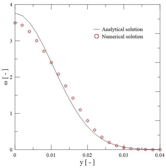
Figure 4.
Diffusion of a vortex sheet—comparison of corrected core-spreading method with analytical solution: M = 30; t = 0.22; Re = 7650; α = 0.80 and νt = 0.0 [36].
4.2. Aircraft Wake Vortices in Ground Effect with Crosswind
In the attempt to simulate vortex interactions and decay in aircraft wakes, values of ground plane length, release height of the primary vortical structures, and wingspan inferred from laboratory observations were adopted [21]. In Figure 1, the ground plane length was chosen as B = 8.0; the release height of the primary counter-rotating vortical structures was h = 2.0; the initial center-to-center distance between primary vortical structures was b = 1.0; the circulation strength was Γ = 1.0; and the initial radius of every primary vortical structure was r0 = 0.1.
The method of Betz [37] was adopted to predict the structure of aircraft vortex wake related to the parameter r0. Betz’s technique is simple and appropriate, although it cannot be applied in configurations of straining interactions between vortices.
The experimental data presented by Liu and Srnsky [21] were utilized in a closed recirculation water tank at a fixed Reynolds number of Re = 7650, where the dissipation of primary vortical structures suffers interference from the tank wall. Another problem is that instantaneous experimental measurement of the center of the moving vortical structure undoubtedly generates some kind of error. These experimental difficulties also motivated the present research to contribute to the literature.
Other adopted numerical parameters were as follows: number of vortex blobs to discretize every primary vortical structure of N = 50; number of flat panels to discretize the ground plane of M = 40; spatial refinement factor of α = 0.80; initial core radius of 0.001; maximum core radius (before of partition) of 0.00125; and minimum vortex strength (before partition) of 0.0004.
Table 1 shows the test cases simulated for the Reynolds number fixed at Re = 7650. The same arrangement of test cases is also simulated for the Reynolds number of Re = 75,000. All test cases were performed with 1000 time steps of magnitude Δt = 0.05.

Table 1.
Physical parameters used in the simulation for Re = 7650. U∞ is the crosswind velocity and ε/Δs is the relative roughness height.
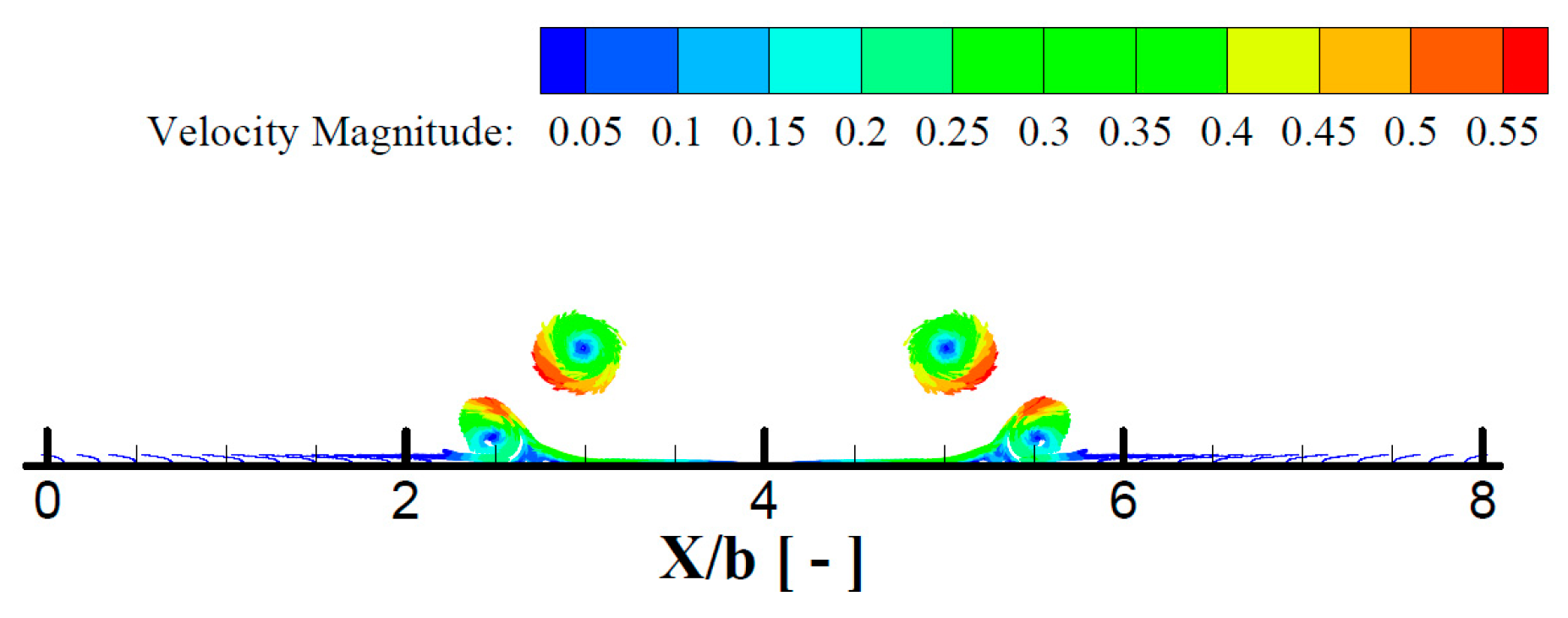
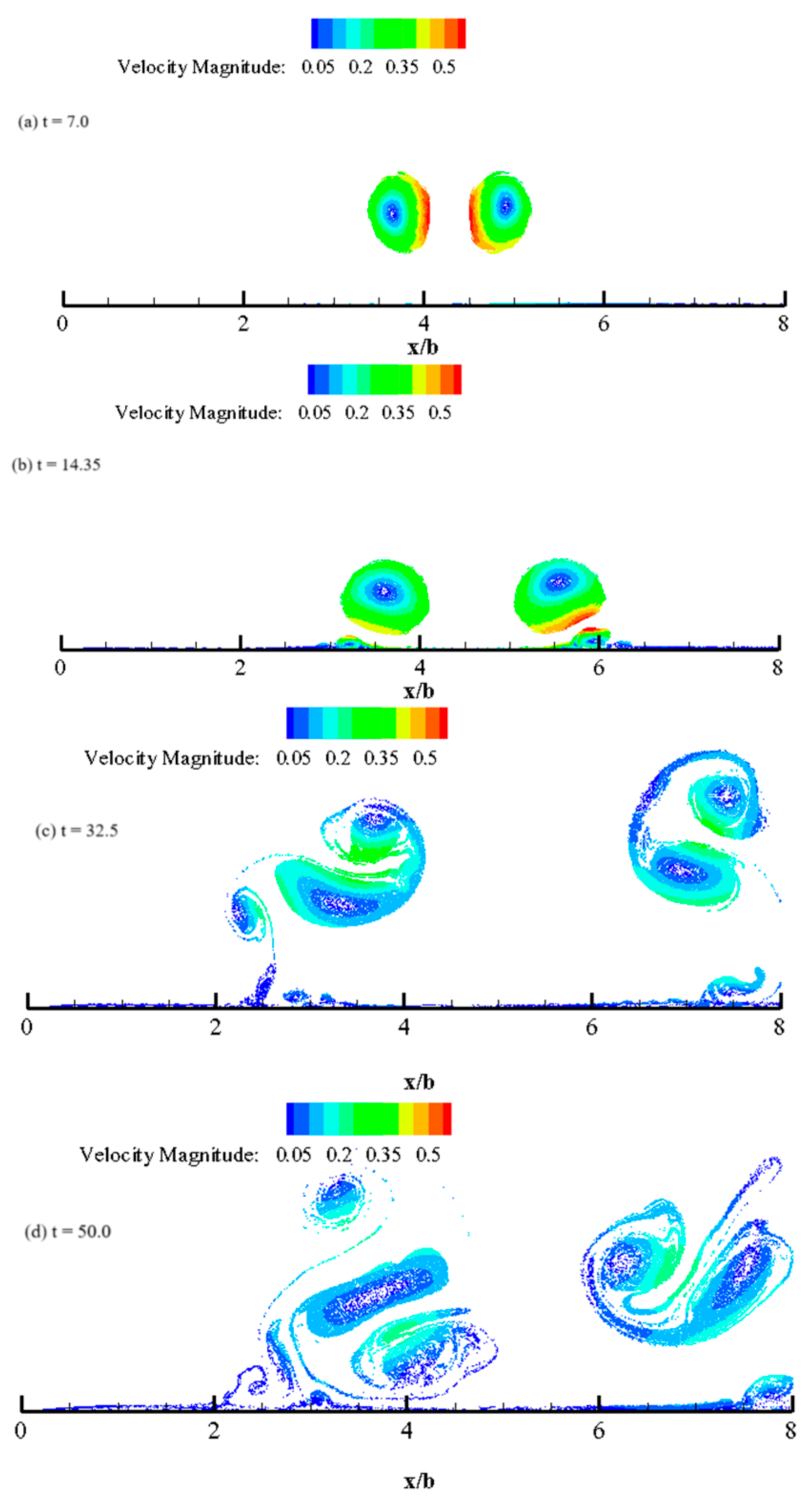
Figure 5 shows the instantaneous behavior of the velocity field during the interaction of the primary vortical structures with the ground plane at time t = 15 (test case 1 in Table 1). The generation of secondary vortical structures from the ground can be successfully identified from Figure 5. Those primary vortical structures will separate and rebound upon interacting with the ground plane. The formation of secondary vortical structures is the key effect responsible for the rebound.

Figure 5.
Instantaneous velocity field distribution: t = 15; Re = 7650, U∞ = 0.0 and ε/Δs = 0.0.
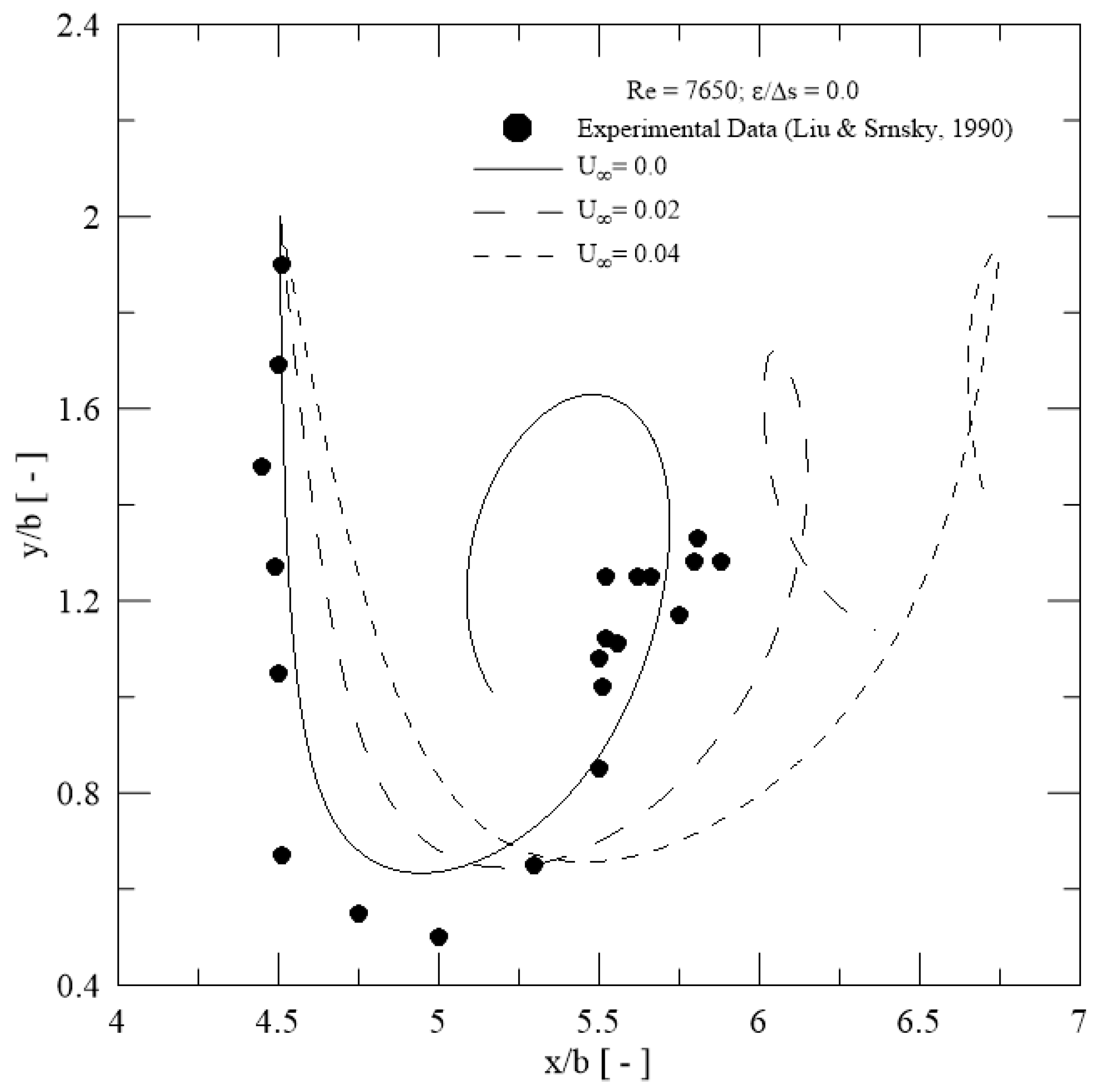
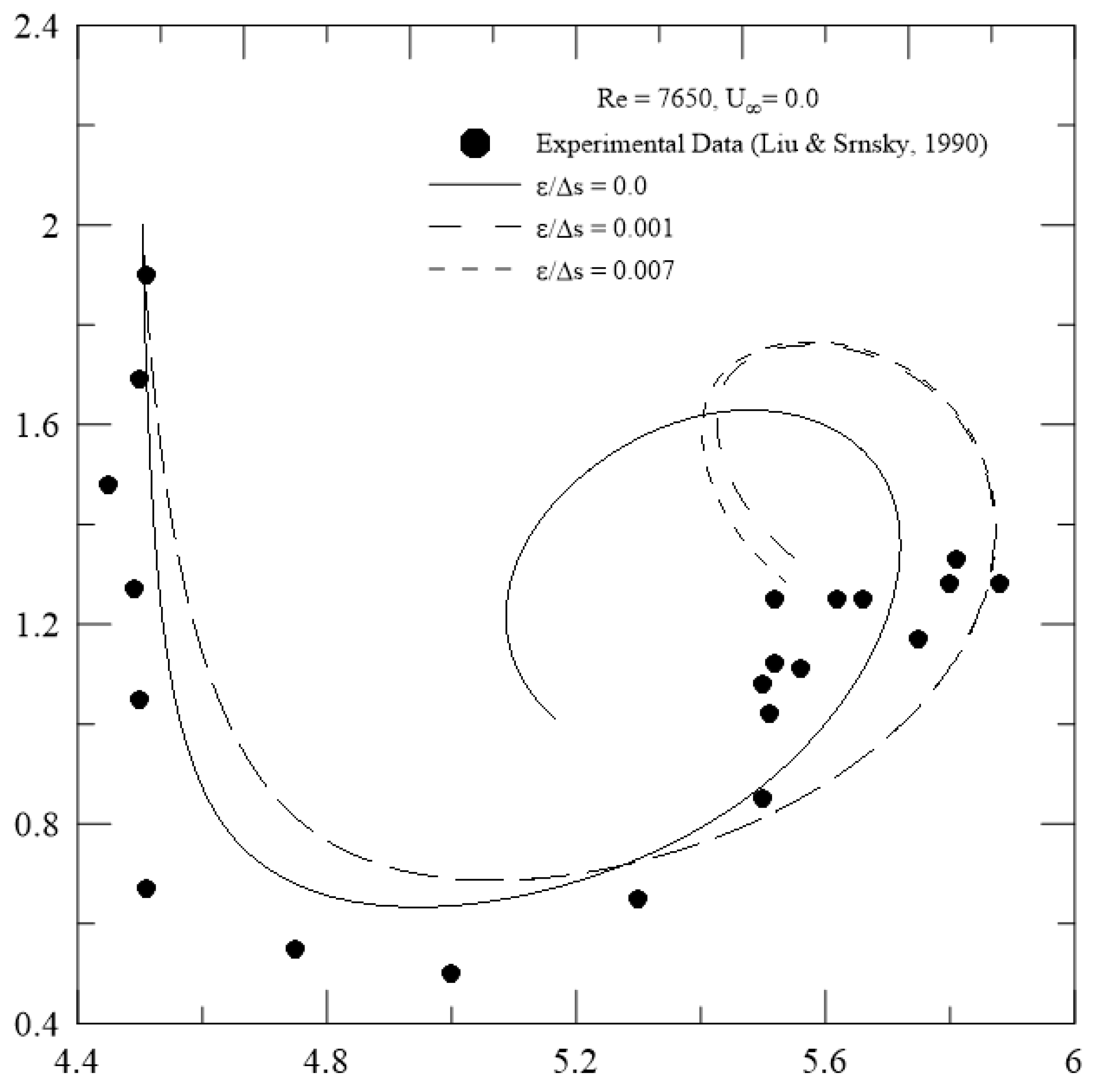
In Figure 1, the centroid of the primary vortical structure from the right is instantaneously computed during the numerical simulation in a typical Lagrangian manner. The numerical value for the centroid is compared with the experimental result measured by Liu and Srnsky [21]. Figure 6 presents comparisons of three numerical trajectories (cases 1, 4, and 7 in Table 1) with the trajectory measured by Liu and Srnsky [21]. The numerical trajectories differ among them, presenting a variation in crosswind velocities, namely U∞ = 0.0, 0.02, and 0.04.
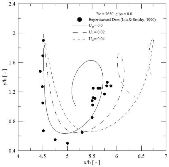
Figure 6.
Comparisons among vortices trajectories with no roughness effects: Re = 7650 [21].
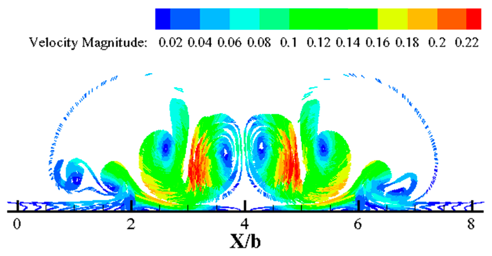
Figure 7 shows that the primary vortical structures, identified in Figure 5 at t = 15, evolved to the last instant of the numerical simulation. During that time interval, the primary vortical structures approach and do not leave the runway. It can be observed in Figure 6 that the centroid of the primary vortical structure from the right attained a maximum height in the order of 0.8 h during the loop, which is clearly a potential hazard to smaller aircraft operating on the same runway. The numerical result indicates that rebounding vortices may relink and even undergo additional rebound. The vortex Reynolds number defined in terms of circulation strength, Γ, and kinematic viscosity, ν, proves suitable for capturing this type physics [21].
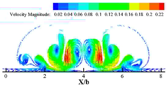
Figure 7.
Instantaneous velocity field distribution: t = 50; Re = 7650, U∞ = 0.0 and ε/Δs = 0.0.
The literature has reported that physics associated with the rebounding effect does not occur unless the viscous boundary layer condition is imposed on the runway [22,23,24,25,26].
Figure 8 shows the phenomena above interpreted including a crosswind velocity of magnitude U∞ = 0.04 blowing the primary vortical structures. It can be concluded that there are crosswinds of sufficient magnitude to counteract the cross-runway displacement of one vortical structure and prevent it from traversing away from the ground plane. Under that condition, it is clear that the potential hazard is for aircraft approaching on the same (or a parallel) runway.

Figure 8.
Instantaneous velocity field distribution: t = 50; Re = 7650, U∞ = 0.04 and ε/Δs = 0.0.
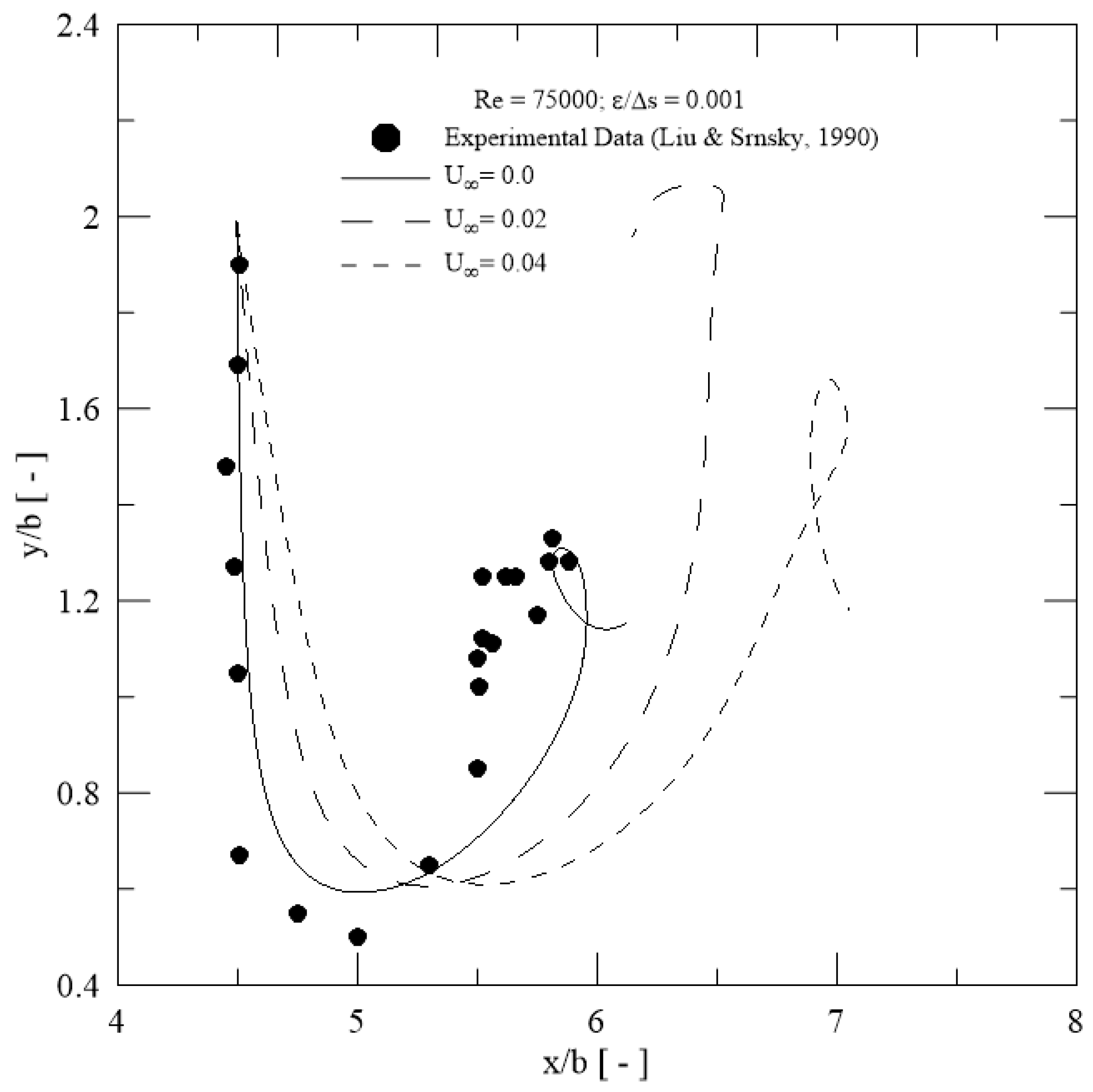
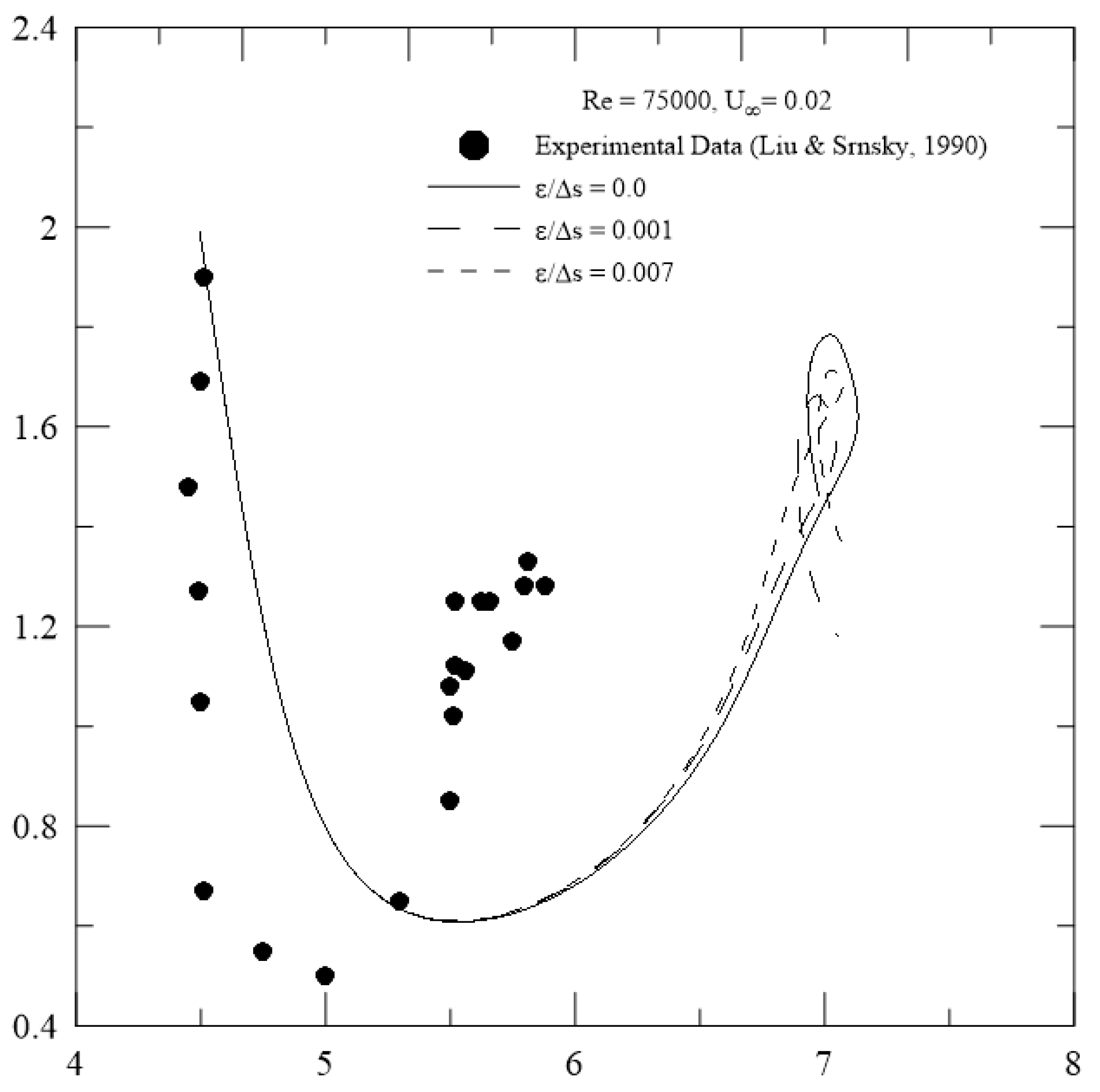
Figure 9 shows trajectories of the centroid of the primary vortical structure from right when the Reynolds number is increased to Re = 75,000. The vortical structure configuration with no crosswind attains a maximum height in the order of 0.9 h during the loop. It can also be concluded that the primary vortical structures survive the interaction with the runway and are blown by crosswinds into the path of another aircraft approaching on the same (or a parallel) runway.
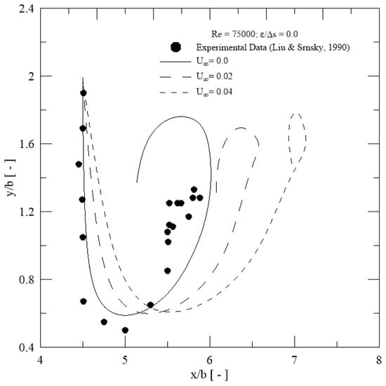
Figure 9.
Comparisons among vortices trajectories with no roughness effects: Re = 75,000 [21].
A comparison between trajectories for crosswind velocity of magnitude U∞ = 0.04 indicates that the vortical structure from the right tends to move faster leaving the runway at Re = 75,000 (Figure 6 and Figure 9 can be compared). Attention should be given to smaller aircraft operating on a parallel runway during the presence of that aircraft wake in the vicinity.
The sensitivity of the roughness model can be captured in Figure 10. When the relative roughness height of ε/Δs = 0.001 is adopted, the main result is that primary vortical structures also survive the interaction with a rough ground plane and can attain a maximum height in the order of 0.95 h during the loop (U∞ = 0.02) at Re = 7650. Interestingly, the configuration with U∞ = 0.04 does not describe the loop leaving the runway any faster (Figure 6 and Figure 10 can be compared). Unfortunately, the experimental data [21] did not include the combined effects of crosswind and surface roughness to be compared.

Figure 10.
Trajectories of wake vortices with roughness effects: Re = 7650 and ε/Δs = 0.001 [21].
The results of the configuration using ε/Δs = 0.001 and Re = 75,000 are shown in Figure 11. When compared with the numerical results in Figure 9, the looping of the primary vortical structure for two crosswind values can be identified. In Figure 11, the vortical structure configuration with a crosswind of magnitude U∞ = 0.02 attains a maximum height in the order of 1.05 h during the loop. Furthermore, the crosswind velocity of magnitude U∞ = 0.04 makes the vortical structure from the right attain a maximum height of about 0.83 h during the loop; consequently, that vortical structure tends to leave the runway faster with sufficient intensity into the path of a smaller aircraft operating on a parallel runway.
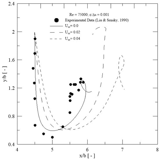
Figure 11.
Trajectories of wake vortices with roughness effects: Re = 75,000 and ε/Δs = 0.001 [21].
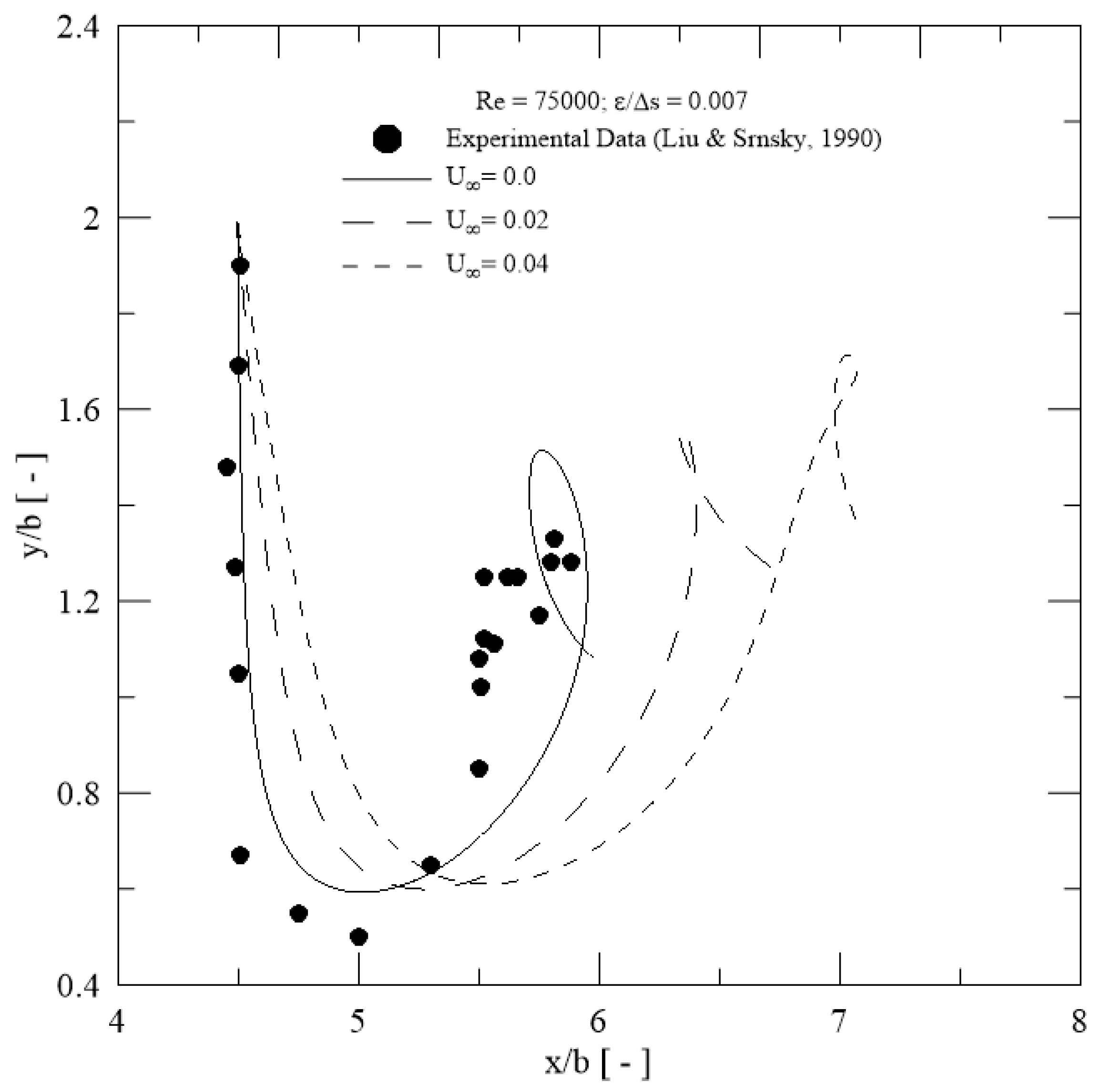
The effects of the higher relative roughness height, i.e., ε/Δs = 0.007, are initially shown in Figure 12 and Figure 13. The most important result for Re = 7650 is that crosswind of magnitude U∞ = 0.04 inhibits the primary vortical structure to loop a distance less than 0.875 B (Figure 12). That behavior can be linked with vertical shear effects because of surface roughness interaction with the primary vortical structures. In practice, the vertical shear provokes a change in the crosswind velocity as a function of the vertical coordinate; consequently, the extent of the rebound is also modified. The roughness effects are also able to change the form of a primary vortical structure without destroying it. The control of roughness height effects is important because the trajectory of primary vortices is quite modified.

Figure 12.
Trajectories of wake vortices with roughness effects: Re = 7650 and ε/Δs = 0.007 [21].
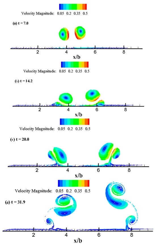
Figure 13.
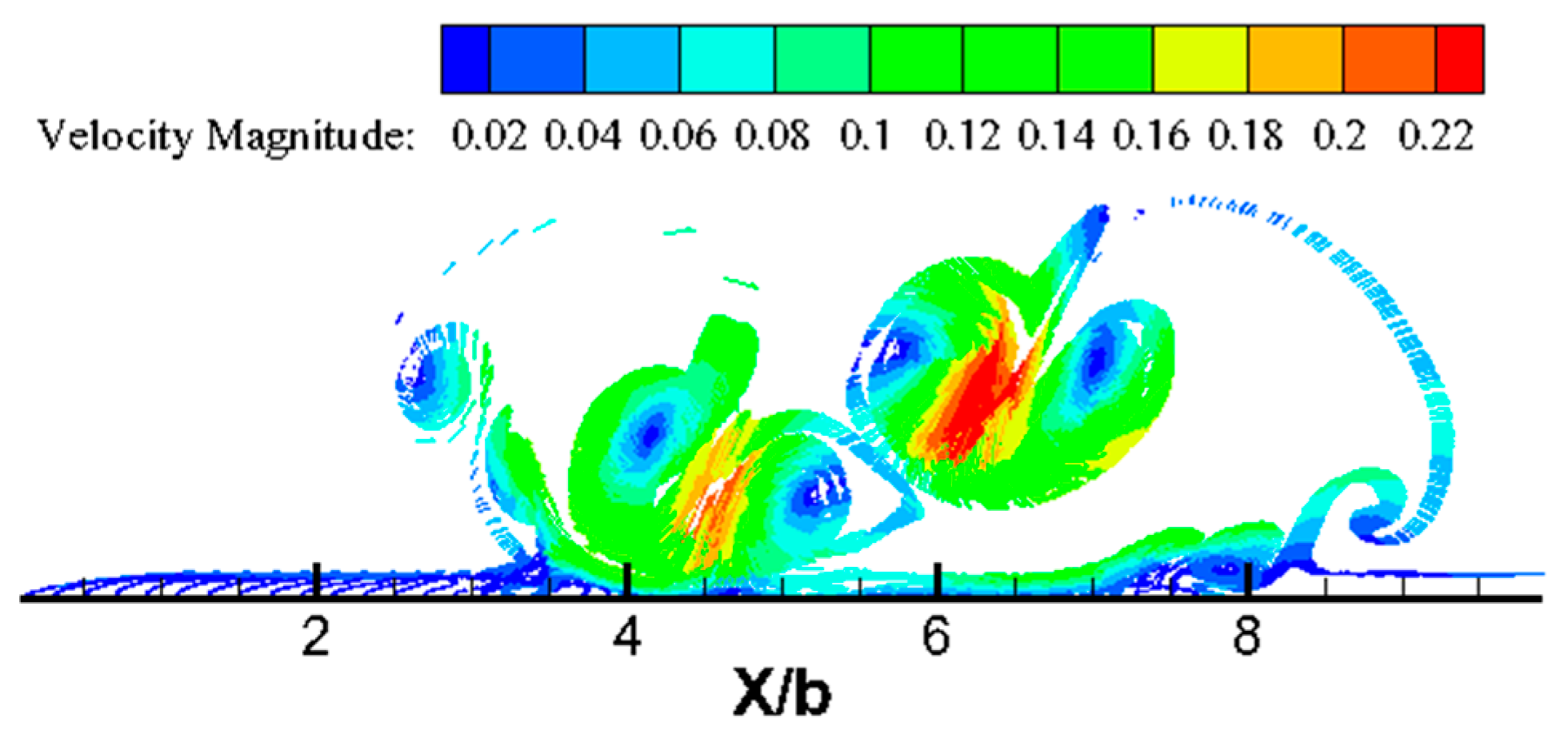
Instantaneous velocity field distributions: Re = 7650, U∞ = 0.04 and ε/Δs = 0.007.
In Figure 13, the time evolution of the pair of primary vortical structures for test case 9 can be accompanied, as shown in Table 1. The interference of the crosswind velocity of magnitude U∞ = 0.04 can be clearly visualized in Figure 13b when compared with Figure 5 (test case 1 in Table 1). The combination of the effects of crosswind with higher velocity and relative roughness with higher height pushes the vortical structures more quickly towards the runway on the right. The decay in wake vortices can also be visualized through numerical values present in the legend “Velocity Magnitude” in Figure 13a–d.
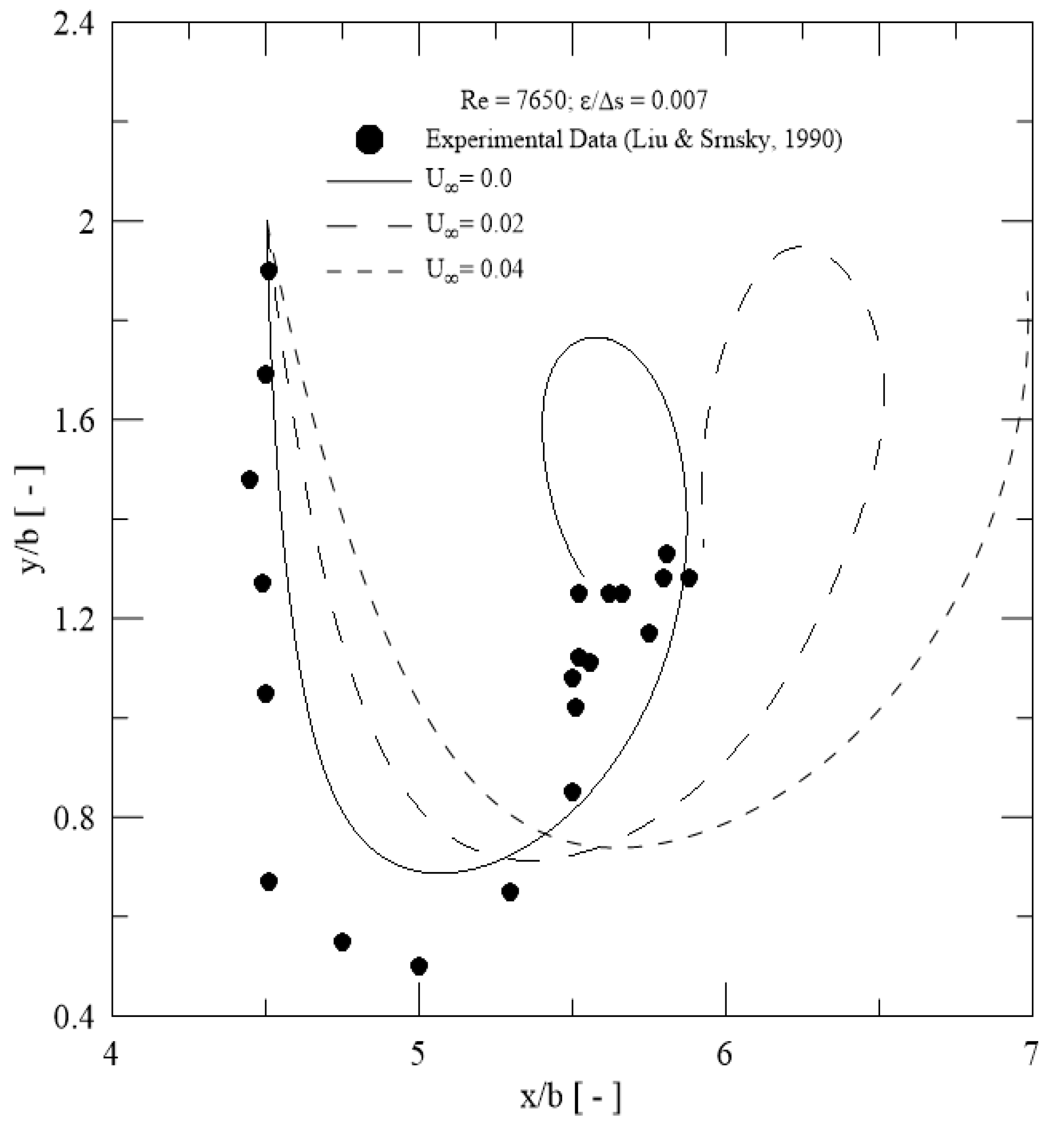
Another interesting result in Figure 14 shows that the combination of crosswind velocity of U∞ = 0.02 with a relative roughness height of ε/Δs = 0.007 at Re = 75,000 restores the condition for the primary vortical structure from right to loop, in which a maximum height of order of 0.78 h is then attained (Figure 11 and Figure 14 can be compared).
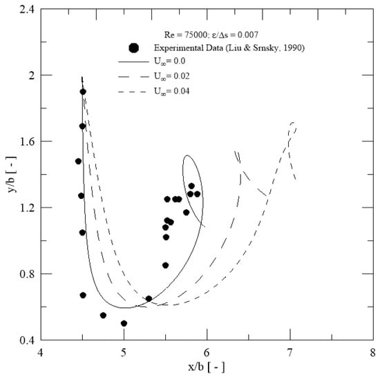
Figure 14.
Trajectories of wake vortices with roughness effects: Re = 75,000 and ε/Δs = 0.007 [21].
An important observation is that decay in wake vortices is much more pronounced than the configuration with no crosswind and a smooth ground plane, when Figure 7 and Figure 15d are compared through the legend “Velocity Magnitude” at t = 50.
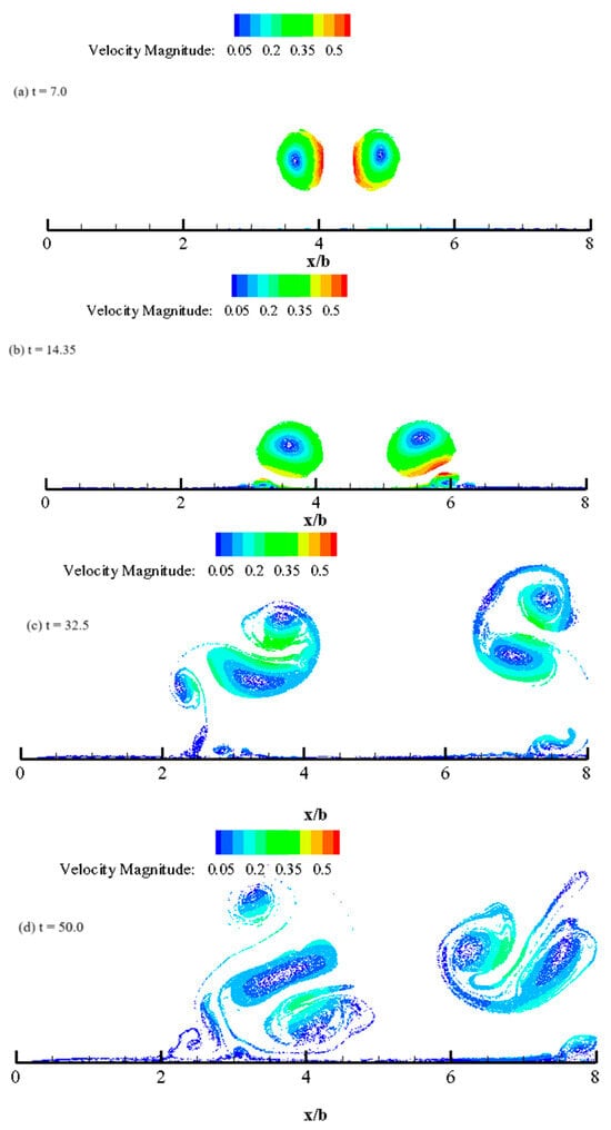
Figure 15.
Instantaneous velocity field distributions: Re = 75,000, U∞ = 0.04 and ε/Δs = 0.007.
In Figure 14, it can be clearly observed that crosswind interference combined with higher relative roughness height makes the loop higher as the crosswind velocity magnitude increases. As a consequence, the vortical structures´ velocity magnitude will also decrease, i.e., the vortical structures encounter less difficulty in leaving the ground plane, being more easily blown by crosswind.
Rough surfaces are proven to be able to control the flow separation of secondary vortical structures originating from the ground plane. Thus, the numerical results shown in Figure 14 seem to indicate that roughness effects are able to move the separation points downstream. Figure 11 and Figure 14, when compared, show that the looping phenomenon in the primary vortical structure from the right and its subsequent movement leaving the runway depend on the features of roughness at a high Reynolds number of Re = 75,000.
The surface roughness interference on the velocity field decay is clearly identified when the Reynolds number increases from Re = 7650 (Figure 13) to Re = 75,000 (Figure 15). The roughness effects are also able to change trajectories because of interactions between vortical structures and the rough ground plane with no crosswind at Re = 7650 (Figure 16).
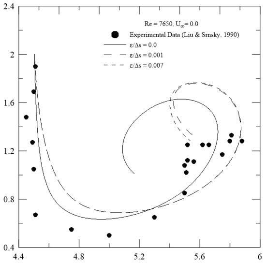
Figure 16.
Trajectories of wake vortices with roughness effects: Re = 7650 and U∞ = 0.0 [21].
The mutual interference between crosswind and surface roughness appears as an important control technique to investigate the potential hazard of aircraft wake vortices at high Reynolds number flows (e.g., Figure 17). Very good knowledge production by researchers is necessary in order to increase airport capacity around the world. The results of analysis of both experimental data and numerical simulations are necessary to elucidate different aspects of nonlinear hydrodynamic phenomena intrinsic to the problem of aircraft wake vortices in terms of the ground effect.
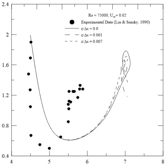
Figure 17.
Trajectories of wake vortices with roughness effects: Re = 75,000 and U∞ = 0.02 [21].
The problem is complex as it involves parameters affected by the vortex-generating aircraft, by vortex-encountering aircraft and by meteorology [25]. Of particular interest here, the motion of wake vortices (generated by a large aircraft) near the rough ground plane with crosswind was investigated to show the potentialities of a Lagrangian vortex method with LES theory, including core spreading and vortex blob splitting.
The use of LES theory allows for solving small-scale lengths in the order of the vortex core radius, namely σ0 = 0.001. As a consequence, the final CPU time for the new scheme implemented using parallel computing (OpenMP) was about 122 min when using an Intel® CoreTM i7-2600 CPU@3.4 GHz. The use of parallel computing is necessary because of the expensive computational cost of the developed algorithm. Thus, the present technique has the following disadvantages: (a) the final CPU time of a typical numerical simulation is particularly long because of the vortex–vortex interaction (the Biot–Savart law), which is computed using Equation (10); (b) the use of the method of images contributes to an increase in the final CPU time, since vortex images have to be considered when using Equation (10); and (c) the core spreading and the vortex blob splitting contribute to an increase in the number of vortex blobs. Therefore, the development of an adaptive, parallel version of the fast multipole method (FMM) [16,17] to the kind of resolution required to treat engineering flows is necessary. The fast multipole method is a technique allowing for the fast computation of long-range interactions between NV vortex blobs in O(NV) or O(NV log NV) steps with some prescribed error tolerance. The Biot–Savart law requires interactions between NV vortex blobs in O(NV2) steps.
As a future study, we also plan to simulate buoyancy forces acting on aircraft wake vortices in the vicinity of a rough ground plane exchanging heat with the fluid flow [30]. For this, the second-order velocity structure function model of the filtered field will be incorporated into the energy equation to capture interaction between particle temperatures and vortex blobs.
5. Conclusions
A Lagrangian vortex method algorithm was developed to blend large-eddy simulation (LES) theory with a surface roughness model. The viscous effects were computed through the corrected core-spreading method, in which vortex blobs were not treated as fluid material particles; otherwise, “convergence errors” would be identified. The local eddy viscosity coefficient was computed together with the vorticity diffusion solution from Equation (12). The local second-order velocity structure function of the filtered field was used to compute the eddy viscosity coefficient from Equation (4), also enabling the implementation of the roughness model from Equation (8). The roughness model once again proves to be efficient since it has already been applied to study bluff body aerodynamics in high Reynolds number flows by Lagrangian vortex method [7,8].
The method was applied to aircraft wake vortices evolving close to the rough ground plane with crosswind. The following conclusions were obtained:
- (i)
- Lagrangian vortex interactions with combined effects of crosswind and surface roughness were efficient in simulating the enhanced dissipation of aircraft vortex wakes in the vicinity of a runway.
- (ii)
- The effect of aircraft wake vortices separating and rebounding upon interacting with the runway was successfully captured.
- (iii)
- The formation of the boundary layer on the ground and the subsequent generation of secondary vortical structures were the key effects responsible for the rebound; thoses phenomena were simulated in a very good physical sense.
- (iv)
- A comparison of trajectories of primary vortical structure between experimental data and numerical results presented a good agreement at Re = 7650 (Figure 6). The experimental data included the effects of the lateral wall for the recirculation water tank.
- (v)
- The crosswind velocity of magnitude U∞ = 0.04 combined with relative roughness height of ε/Δs = 0.001 at Re = 75,000 caused the primary vortical structure to attain a maximum height of about 0.83 h during the loop; importantly, vortical structures tend to leave the runway faster with sufficient intensity to disturb a smaller aircraft operating on a parallel runway (Figure 11).
- (vi)
- (vii)
- The control of roughness height appeared to be a determining factor to interfere with the trajectory of primary vortices generated by a large aircraft approaching or leaving a ground plane with crosswind.
- (viii)
- The numerical results confirmed that extensive data and CFD are required to develop wake models linked with systems such as “Wake Turbulence Re-categorization or Wake RECAT” (a safe decrease in separation standards between aircrafts).
Author Contributions
Conceptualization, G.F.M.d.C., M.F.V. and L.A.A.P.; data curation, G.F.M.d.C., M.F.V. and A.M.B.; formal analysis, G.F.M.d.C., A.M.B. and L.A.A.P.; funding acquisition, L.A.A.P.; investigation, G.F.M.d.C., M.F.V. and A.M.B.; methodology, A.M.B. and L.A.A.P.; project administration, G.F.M.d.C. and L.A.A.P.; resources, G.F.M.d.C. and L.A.A.P.; software using Fortran, G.F.M.d.C. and M.F.V.; validation, G.F.M.d.C., M.F.V. and A.M.B.; visualization, G.F.M.d.C. and L.A.A.P.; supervision, L.A.A.P.; writing—original draft, L.A.A.P.; and writing—review and editing, G.F.M.d.C., A.M.B. and L.A.A.P. All authors have read and agreed to the published version of the manuscript.
Funding
The authors would like to thank FAPEMIG (a research supporting foundation of Minas Gerais state), project no. APQ-01246-23; and the São Paulo Research Foundation (FAPESP), grant no. 2022/03630-4, for their financial support.
Institutional Review Board Statement
Not applicable.
Informed Consent Statement
Not applicable.
Data Availability Statement
The data presented in this study are available on request from the corresponding author. The data are not publicly available due to privacy and ethical restrictions.
Conflicts of Interest
The authors declare no conflict of interest.
References
- Reynolds, O. An Experimental Investigation of the Circumstances Which Determine Whether the Motion of Water shall be Direct or Sinuous, and of the Law of Resistance in Parallel Channels. Proc. R. Soc. Lond. 1883, 35, 84. [Google Scholar]
- Ozkan, G.M.; Egitmen, H. Turbulent Structures in an Airfoil Wake at Ultra-Low to Low Reynolds Numbers. Exp. Therm. Fluid Sci. 2022, 134, 110622. [Google Scholar] [CrossRef]
- Sporschill, G.; Billard, F.; Mallet, M.; Manceau, R.; Bézard, H. Assessment of Reynolds-Stress Models for Aeronautical Applications. Int. J. Heat. Fluid Flow. 2022, 96, 108955. [Google Scholar] [CrossRef]
- List, B.; Chen, L.; Thuerey, N. Learned Turbulence Modelling with Differentiable Fluid Solvers: Physics-Based Loss Functions and Optimisation Horizons. J. Fluid Mech. 2022, 949, A25. [Google Scholar] [CrossRef]
- Alcântara Pereira, L.A.; Hirata, M.H.; Silveira Neto, A. Vortex Method with Turbulence Sub-grid Scale Modeling. J. Braz. Soc. Mech. Sci. Eng. 2003, 25, 140–146. [Google Scholar]
- Hirata, M.H.; Alcântara Pereira, L.A.; Recicar, J.N.; Moura, W.H. High Reynolds Number Oscillations of a Circular Cylinder. J. Braz. Soc. Mech. Sci. Eng. 2008, 30, 368. [Google Scholar] [CrossRef]
- Bimbato, A.M.; Alcântara Pereira, L.A.; Hirata, M.H. Development of a New Lagrangian Vortex Method for Evaluating Effects of Surfaces Roughness. Eur. J. Mech. B Fluids 2019, 74, 291–301. [Google Scholar] [CrossRef]
- Moraes, P.G.; Alcântara Pereira, L.A. Surface Roughness Effects on Flows past Two Circular Cylinders in Tandem Arrangement at Co-shedding Regime. Energies 2021, 14, 8237. [Google Scholar] [CrossRef]
- Kamemoto, K. On Contribution of Advanced Vortex Element Methods toward Virtual Reality of Unsteady Vortical Flows in the New Generation of CFD. J. Braz. Soc. Mech. Sci. Eng. 2004, 26, 368–378. [Google Scholar] [CrossRef]
- Mimeau, C.; Mortazavi, I. A Review of Vortex Methods and Their Applications: From Creation to Recent Advances. Fluids 2021, 6, 68. [Google Scholar] [CrossRef]
- Martensen, E. Berechnung und Simulation der Beanspruchung einer Fußbodensitzschiene einschließlich Krafteinleitung. Arch. Rat. Mech. 1959, 3, 235–270. [Google Scholar] [CrossRef]
- Chorin, A.J. Numerical Study of Slightly Viscous Flow. J. Fluid Mech. 1973, 57, 785–796. [Google Scholar] [CrossRef]
- Leonard, A. Vortex Methods for Flow Simulations. J. Comput. Phys. 1980, 37, 289–335. [Google Scholar] [CrossRef]
- Greengard, C. The Core Spreading Vortex Method Approximate the Wrong Equation. J. Comp. Phys. 1985, 61, 345–348. [Google Scholar] [CrossRef]
- Rossi, L.F. Resurrecting Core Spreading Vortex Methods: A New Scheme that is Both Deterministic and Convergent. SIAM J. Sci. Comput. 1996, 17, 370–397. [Google Scholar] [CrossRef]
- Yokota, R.; Narumi, T.; Sakamaki, R.; Kameoka, S.; Obi, S.; Yasuoka, K. Fast Multipole Methods on a Cluster of GPUs for the Meshless Simulation of Turbulence. Comput. Phys. Commun. 2009, 180, 2066–2078. [Google Scholar] [CrossRef]
- Salloum, S.; Lakkis, I. An Adaptive Error-Controlled Hybrid Fast Solver for Regularized Vortex Methods. J. Comput. Phys. 2022, 468, 111504. [Google Scholar] [CrossRef]
- Marchevsky, I.; Ryatina, E.; Kolganova, A. Fast Barnes-Hut-Based Algorithm in 2D Vortex Method of Computational Hydrodynamics. Comput. Fluids 2023, 266, 106018. [Google Scholar] [CrossRef]
- Xiong, S.; He, X.; Tong, Y.; Deng, Y.; Zhu, B. Neural Vortex Method: From Finite Lagrangian Particles to Infinite Dimensional Eulerian Dynamics. Comput. Fluids 2023, 258, 105811. [Google Scholar] [CrossRef]
- Lesieur, M.; Métais, O. New Trends in Large Eddy Simulation of Turbulence. Rev. Fluid Mech. 1996, 28, 45–82. [Google Scholar] [CrossRef]
- Liu, H.T.; Srnsky, R.A. Laboratory Investigation of Atmospheric Effects on Vortex Wakes; Report, No. 497; Flow Research, Inc.: Belleville, ON, Canada, 1990. [Google Scholar]
- Vyshinsky, V.V. Aircraft Vortex Wake and Airport Capacity. J. Aerosp. 1997, 106, 1381–1393. Available online: https://www.jstor.org/stable/44650529 (accessed on 28 September 2023).
- Bobylev, A.V.; Vyshinsky, V.V.; Soudakov, G.G.; Yaroshevsky, V.A. Aircraft Vortex Wake and Flight Safety Problems. J. Aircr. 2010, 47, 663–674. [Google Scholar] [CrossRef]
- Vechtel, D.; Stephan, A.; Holzäpfel, F. Simulation Study of Severity and Mitigation of Wake-Vortex Encounters in Ground Proximity. J. Aircr. 2017, 54, 1802–1813. [Google Scholar] [CrossRef]
- Hallock, J.N.; Holzäpfel, F. A Review of Recent Wake Vortex Research for Increasing Airport Capacity. Prog. Aerosp. Sci. 2018, 98, 27–36. [Google Scholar] [CrossRef]
- Critchley, J.B.; Foot, P.B. United Kingdom Civil Aviation Authority Wake Vortex Database; Analysis of Incidents Reported between 1982 and 1990; CAA Paper 91015; CAA: London, UK, 1991. [Google Scholar]
- Holzäpfel, F.; Strauss, L.; Schwarz, C. Assessment of Dynamic Pairwise Wake Vortex Separations for Approach and Landing at Vienna Airport. Aerosp. Sci. Technol. 2021, 112, 106618. [Google Scholar] [CrossRef]
- Xu, Z.; Li, D.; An, B.; Pan, W. Enhancement of Wake Vortex Decay by Air Blowing from the Ground. Aerosp. Sci. Technol. 2021, 118, 107029. [Google Scholar] [CrossRef]
- Xu, Z.; Li, D.; Cai, J. Long-Wave Deformation of In-Ground-Effect Wake Vortex Under Crosswind Condition. Aerosp. Sci. Technol. 2023, 142, 108697. [Google Scholar] [CrossRef]
- Moraes, P.G.; Oliveira, M.A.; Bimbato, A.M.; Alcântara Pereira, L.A. A Lagrangian Description of Buoyancy Effects on Aircraft Wake Vortices from Wing Tips near a Heated Ground Plane. Energies 2022, 15, 6995. [Google Scholar] [CrossRef]
- Kundu, P.K. Fluid Mechanics; Academic Press: Cambridge, MA, USA, 1990. [Google Scholar]
- Katz, J.; Plotkin, A. Low Speed Aerodynamics: From Wing Theory to Panel Methods; McGraw Hill Inc.: New York, NY, USA, 1991. [Google Scholar]
- Kelvin, L. On vortex motion. Trans. Roy. Soc. Edin. 1869, 25, 217–260. [Google Scholar]
- Helmholtz, H. On integrals of the hydrodynamic equations which express vortex motions. Philos. Mag. 1867, 33, 485. [Google Scholar] [CrossRef]
- Ferziger, J.H. Numerical Methods for Engineering Application; John Wiley & Sons, Inc.: Hoboken, NJ, USA, 1981. [Google Scholar]
- Batchelor, G.K. An Introduction to Fluid Dynamics; Cambridge University Press: Cambridge, UK, 2000. [Google Scholar]
- Betz, A. Behavior of Vortices Systems; NACA TM 713; trans. from ZAMM, XII, 3, June 1932; NASA: Washington, DC, USA, 1933. [Google Scholar]


Disclaimer/Publisher’s Note: The statements, opinions and data contained in all publications are solely those of the individual author(s) and contributor(s) and not of MDPI and/or the editor(s). MDPI and/or the editor(s) disclaim responsibility for any injury to people or property resulting from any ideas, methods, instructions or products referred to in the content. |
© 2023 by the authors. Licensee MDPI, Basel, Switzerland. This article is an open access article distributed under the terms and conditions of the Creative Commons Attribution (CC BY) license (https://creativecommons.org/licenses/by/4.0/).