Integrated Dynamic Model for Numerical Modeling of Complex Landslides: From Progressive Sliding to Rapid Avalanche

Featured Application

An integrated dynamic model has been proposed, which can be used to analyze landslides with significant changes in dynamic characteristics due to changes in the integrity of the landslide mass. The analysis results can be directly applied to landslide prevention and mitigation applications based on geographic information systems (GIS).

Abstract

Landslides are one of the most common catastrophic mass flows in mountainous areas. The occurrence of fragmentation leads to the evolution of the integrity and stiffness of the sliding mass. The changes in internal composition caused by basal erosion and entrainment make the dynamic evolution of landslides more complex. To consider these complex processes, physics-based dynamic models are often used to analyze the dynamic characteristics of landslides. However, the proprietary assumptions of dynamic models often limit their application to complex events. A single dynamic model is often not competent for the analysis of landslides with evolving dynamic characteristics. In this study, two dynamic models are effectively integrated according to the evolving characteristics of the landslide. The common effects of basal erosion and entrainment are also considered. The maximum sliding velocity, accumulation range, and erosion depth characteristics of this integrated dynamic model are more consistent with the field than those of the single dynamic model. Under the terrain conditions of this study, within a few seconds of the triggering stage, if the occurrence of disintegration is advanced by 2 s, the maximum impact area will increase by about 3.1% to 4.1%, and the maximum kinetic energy will increase by more than 20%. Simulation results indicate that the changes in the integrity of the landslide body significantly affect the evolution of subsequent landslide dynamic characteristics.

1. Introduction

Landslides are common geological disasters in mountainous areas that pose serious threats to human life, property, and the natural environment [1,2,3]. Landslides can involve complex evolutions of dynamic characteristics of the mobile mass, such as the traveled distance, velocity, and extent of affected areas. Evaluation of the runout dynamic characteristics of landslides has significant geotechnical significance, especially in landslide hazard assessment or identifying potential mitigation measures [4,5,6,7].

Various methods have been proposed for landslide runout analysis, which can be categorized into empirical–statistical and analytical methods [3]. The empirical–statistical methods are typically based on observations to establish correlations between the characteristics of the source area and the runout behaviors (e.g., [8,9,10]). Analytical methods are mainly based on the analysis of landslide physical processes and can be categorized into numerical (dynamic) methods [1,11,12,13] and closed analytical equations. The application of the statistical method is limited by the representativeness of source area features, and the accuracy of the method is affected by the amount of statistical data. In contrast, the dynamic methods, which are based on physical process analysis, can better reproduce the real process of landslides via numerical simulation and provide more dynamic information about landslides [3,6].

Dynamic models with simplified rigid body assumptions have been proposed early, such as the mass point method (or lumped mass model) [14,15] or the energy-based approach of Körner [16]. All these methods assume that the entire mass is concentrated at the centroid of the landslide body. During the analysis, the internal deformation of the sliding mass will be ignored, so these models are more suitable for analyzing landslides with high integrity. After that, methods using the deformable hypothesis were proposed. In these methods, a sliding body will be discretized into deformable blocks adjacent to each other [17] or rigid bodies connected by springs, through which the deformation of the block can be approximated equivalently [18,19]. These methods are suitable for analyzing slopes with high initial integrity and whose integrity has not experienced a significant decline during sliding.

In the field of geophysical mass flow, Savage and Hutter [20] proposed the first depth-averaged model for analyzing the avalanches of dry granular mass. Its extended model takes into account the influence of complex terrain and other factors [21,22]. The depth-averaged dynamic models have been extended to solid-fluid two-phase flow [1,12,13], two-layer flow [13,23], two-fluid flow [24], and multiphase flow [25]. For dry landslides with low integrity or high mobility landslides with high water content, the models based on hydrodynamics are more suitable.

Most depth-averaged models are based on hydrodynamics [26]. They ignore the stiffness of sliding materials and assume that landslides become fluidized instantly when failure occurs [27]. Some landslides move like a rigid block at the initial stage and then disintegrate into a flow-like debris avalanche progressively due to friction and vibration [28,29]. In these cases, the application of the depth-averaged model often results in an excessive impact area at the initial stage [3,30,31,32]. In order to obtain results closer to the field within the same dynamic model, some researchers (e.g., [33]) used zone-wised parameter values at the initiation, avalanche, and accumulation zones. However, due to the limitations of the model’s own characteristics, the differences in dynamic characteristics that can be reflected by adjusting parameter values are limited. To overcome this issue, Aaron and Hungr [32] developed a modified version of DAN3D that allows for delaying fluidization based on a user-specified index. They treat the landslide mass as a coherent body until it reaches a certain distance, at which point the depth-averaged model based on hydrodynamics will take over, and then the mass spreading will become apparent.

The erosion and entrainment of bed materials are complex processes depending on the density, strength, and saturation of materials from both the landslide path and the landslide body [34,35,36]. There are huge potential needs for quantitative prediction methods accounting for these important processes [27,36,37,38,39].

To consider the influence of mass integrity on dynamic characteristics, two different dynamic models were effectively integrated in this study. In the early stages, the sliding mass with high integrity was simulated by a multi-block model, which is characterized by low diffusivity. A depth-averaged model will be used for sliding mass with deteriorated integrity and enhanced diffusion due to collisions. In the later stage, the erosion and entrainment effects of substrate materials will be obvious, so both of these effects should be considered in the integrated model [27]. In the following content, we will introduce the multi-block model and the depth-averaged model, respectively. Then, the integration method of the two dynamic models will be introduced. Finally, the validation of the integrated model is carried out by comparing the simulation results with the fields of a real landslide. It is worth pointing out that the executions of all these models are based on the global rectangular coordinate system, which means the data of the digital elevation model (DEM) can be used directly by the integrated model, and the results can also be directly used by GIS-based applications, such as for the spatial prediction of landslide susceptibility [40] and hazard prediction [7,41]. The effectiveness of the integrated dynamic model in analyzing landslides with significant dynamic characteristic changes will be verified by field data. The differences in dynamic characteristics caused by the differences in fragmentation time will be analyzed. The erosion depth calculated via a simple erosion model will also be verified. All of these analyses provide references for landslide runout analysis under similar engineering conditions.

2. Physically Based Dynamic Models for Modeling Complex Landslides

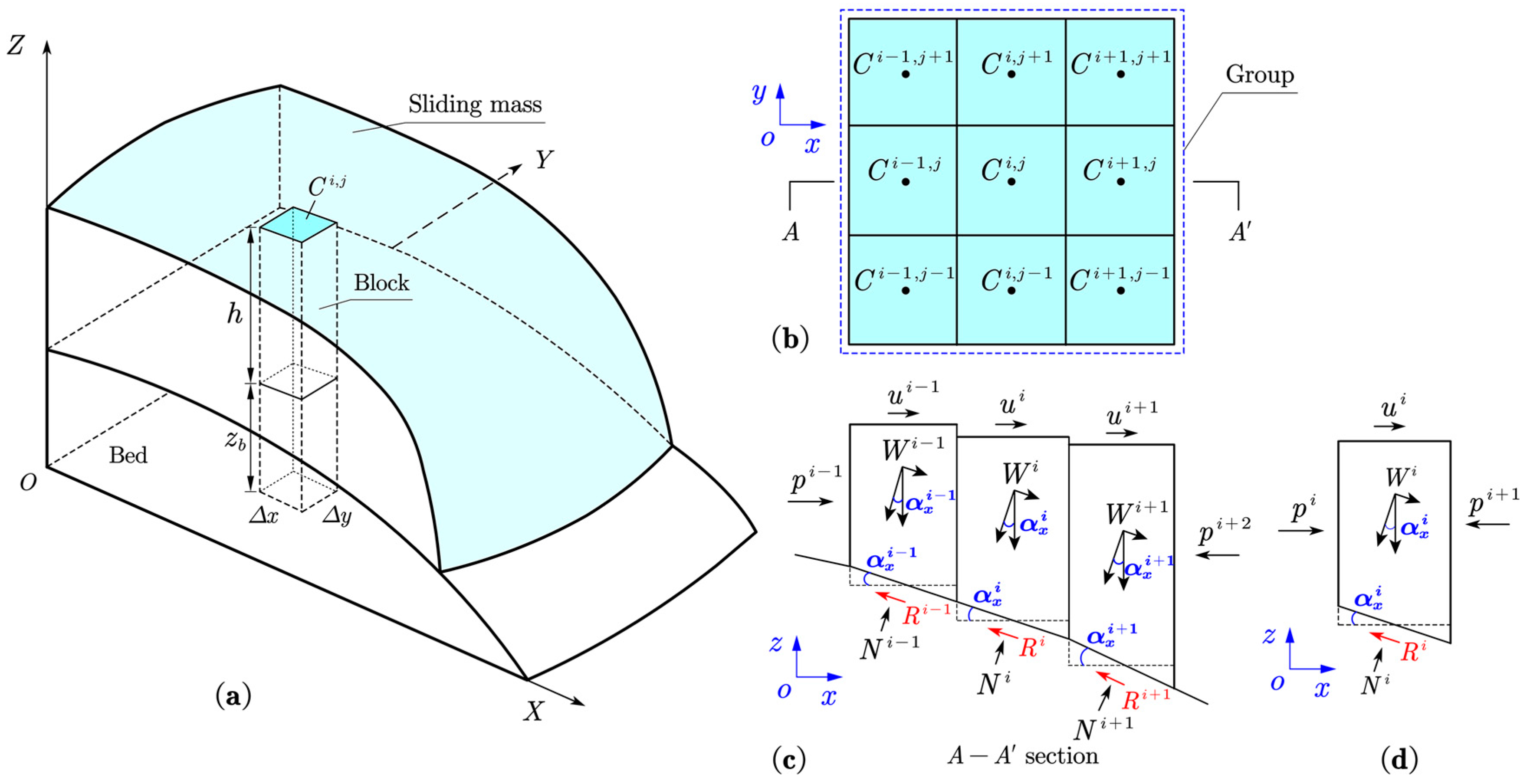
2.1. A Multi-Block Model for Slowly Sliding Landslide

2.1.1. Basic Assumptions

The displacement of sliding masses with high integrity develops slowly in the early stages, and the deterioration of their integrity can be ignored. Thus, at this stage, the landslide can be approximated as a series of rigid blocks that are close to each other (Figure 1a). Each block is subjected to a combined action of sliding and anti-sliding forces. A block (C_i,j) in physical space (Figure 1a) corresponds to a grid cell in the Digital Elevation Model (DEM) (Figure 1b). The entire landslide can be discretized into a numerical model with fixed-size cells, each of which contains physical information, such as the mass (m), fluid height (h), elevation of basal terrain (z_b), velocity, and stress about the landslide (Figure 1c,d).

In Figure 2, the red arrow marked by n is the normal direction of the tangent plane, and its intersection angle with the positive direction of the z-axis is denoted by θ. The intersection angle θ between the normal vector n and the global Z-axis is less than 90° for most terrain, and the corresponding value of n_z will be positive in these cases. The angles between the tangent plane and the x-axis and y-axis are denoted by α_x and α_y in the vertical plane. The elevation function of the basal terrain can be defined as f (x, y, z) = z − z_b (x, y) = 0, which can obtain the elevation values of the cells from the digital elevation model (DEM) in applications. The elevation, as a scalar, is defined at the center of the cells. The accuracy of terrain function data generally depends on the resolution of the DEM.

The normal vector n of the tangent plane passing through any point on the terrain (Figure 2) can be expressed as [19]

$$\mathbf{n}=\left(n_x,n_y,n_z\right)=\frac{\left(-\partial z_b/\partial x,-\partial z_b/\partial y,1\right)}{{\left[{\left(\partial z_b/\partial x\right)}^2+{\left(\partial z_b/\partial y\right)}^2+1\right]}^{1/2}},$$

(1)

From Equation (1), we can obtain

$$n_z=\mathrm{c}\mathrm{o}\mathrm{s}\theta =\frac{1}{{\left[{\left(\partial z_b/\partial x\right)}^2+{\left(\partial z_b/\partial y\right)}^2+1\right]}^{1/2}},$$

(2)

After substituting the geometric relationship, namely tanα_x = ∂z_b/∂x and tanα_y = ∂z_b/∂y, into Equation (2), we obtain

tan²θ = tan²α_x + tan²α_y,

(3)

Therefore, intersection angle θ can be determined via the tangent values of α_x and α_y, which can be obtained directly using the digital elevation model (DEM). The central difference method can be used to calculate these tangent values in the x and y directions:

$$\mathrm{t}\mathrm{a}\mathrm{n}{\alpha }_x^{i,j}=\frac{\partial z_b}{\partial x}=\frac{z_b^{i+1,j}-z_b^{i-1,j}}{2\mathsf{\Delta }x},$$

(4)

$$\mathrm{t}\mathrm{a}\mathrm{n}{\alpha }_y^{i,j}=\frac{\partial z_b}{\partial y}=\frac{z_b^{i,j+1}-z_b^{i,j-1}}{2\mathsf{\Delta }y},$$

(5)

where Δx and Δy are the cell sizes of DEM in the x and y directions, respectively. The superscripts i and j denote the cell indexes in the x and y directions (Figure 1b).

2.1.2. Motion Equations of Gravity-Driven Sliding Blocks

The main factors affecting block motion include gravity, W; anti-sliding force, R; and the interaction forces between blocks, P. The effect of vertical shear stress between blocks was ignored due to their small values. Self-weight is the main driving force that causes the mass to slide. The anti-sliding factor is mainly due to the friction at the basal terrain. It is assumed that the resultant horizontal stress, P, of a block results from the difference in lateral earth pressure acting on both sides of the block (Figure 1d). For granular materials, the resultant horizontal stress vector can be expressed as

$$\mathbf{P}=\mathbf{k}\nabla \left(\rho gh\right),$$

(6)

where $\nabla =\left(\partial /\partial x,\partial /\partial y\right)$ is the gradient operator, and k = (k_x, k_y) is the vector of the lateral earth pressure coefficients [26].

It is assumed that the Coulomb friction law should be obeyed when the block slides along the basal terrain. Then, the net force for a block can be expressed as [42]

$$\mathbf{F}=\left(\mathbf{g}·\mathbf{n}\right)\mathbf{n}-\frac{\mathbf{u}}{\mid \mathbf{u}\mid }\left(\mathbf{g}·\mathbf{n}\right)\mathrm{t}\mathrm{a}\mathrm{n}\delta -\mathbf{k}\nabla \left(\rho gh\right),$$

(7)

where δ is the basal friction angle between the landslide and basal terrain.

From Equation (7), the acceleration components of a block with unit weight in x and y directions can then be derived:

$$a_x=g\mathrm{s}\mathrm{i}\mathrm{n}{\alpha }_x-\frac{u_x}{\mid \mathbf{u}\mid }\left(g\mathrm{c}\mathrm{o}\mathrm{s}\theta \mathrm{t}\mathrm{a}\mathrm{n}\delta \right)-k_x\frac{\partial h}{\partial x},$$

(8)

$$a_y=g\mathrm{s}\mathrm{i}\mathrm{n}{\alpha }_y-\frac{u_y}{\mid \mathbf{u}\mid }\left(g\mathrm{c}\mathrm{o}\mathrm{s}\theta \mathrm{t}\mathrm{a}\mathrm{n}\delta \right)-k_y\frac{\partial h}{\partial y},$$

(9)

where a_x and a_y represent the acceleration components in the x and y directions, respectively. Due to the assumption of unit weight, the product term $\rho g$ disappears from the third term on the right-hand side of Equations (8) and (9).

At the initial stage of sliding, the landslide maintains high integrity, and its internal relative displacement is small. A large portion of the slope has almost the same displacement. For landslides, the grid size of a digital topographic map (DEM) may be at the meter level, while the characteristic size of a block with approximate displacement may be on the scale of tens of meters. This scale range may include multiple cells in the digital terrain model. Therefore, the initial landslide can be divided into several groups, and all the cells in each group have the same velocity characteristics, which is closer to the displacement characteristics of the real landslide. For example, in Figure 1b, one group consists of nine blocks, and the actual number of blocks may be less than this in the irregular margin of the landslide.

Since all blocks within a group should have consistent physical quantities, the overall acceleration component of the group can be viewed as the averaged acceleration components of each block within the group. For example, when a group consists of nine blocks, the averaged angle between the tangent plane of the basal bed and the x and y axes can be expressed as

$${\alpha }_x=\mathrm{a}\mathrm{r}\mathrm{c}\mathrm{t}\mathrm{a}\mathrm{n}\left({\sum }_{i=1}^9\left(h_i\mathrm{t}\mathrm{a}\mathrm{n}{\alpha }_x^i\right)/{\sum }_{i=1}^9{h}_i\right),$$

(10)

$${\alpha }_y=\mathrm{a}\mathrm{r}\mathrm{c}\mathrm{t}\mathrm{a}\mathrm{n}\left({\sum }_{j=1}^9\left(h_j\mathrm{t}\mathrm{a}\mathrm{n}{\mathsf{\alpha }}_y^j\right)/{\sum }_{j=1}^9{h}_j\right),$$

(11)

where the tangent values of the basal terrain of individual blocks can be obtained from Equations (4) and (5).

The last term on the right side of Equations (8) and (9) can also be derived from the average method within the group, which takes the flow depth as the weight as follows:

$$\frac{\overline{\partial h}}{\partial x}=\frac{\sum (h_i\partial h_i/\partial x)}{\sum h_i},$$

(12)

$$\frac{\overline{\partial h}}{\partial y}=\frac{\sum (h_j\partial h_j/\partial y)}{\sum h_j},$$

(13)

For simplicity of presentation, the summation range in Equations (12) and (13) has been dropped. The average acceleration component of each group can be obtained by substituting the average quantity represented by Equations (10)–(13) into Equation (7).

The acceleration can be assumed to be constant within each time increment Δt when the time step is small enough. Then, the new velocity of each block after the incremental time Δt can be expressed as

u_t+∆t = u_t + a_x ∆t,

(14)

v_t+∆t = v_t + a_y ∆t,

(15)

Thereafter, the new displacement of each block within a group can be calculated based on the group-averaged velocity component at the start (t) and end (t + Δt) of the time step:

$$x_{t+\mathsf{\Delta }t}=x_t+\frac{u_t+u_{t+\mathsf{\Delta }t}}{2}\mathsf{\Delta }t\mathrm{c}\mathrm{o}\mathrm{s}{\alpha }_x,$$

(16)

$$y_{t+\mathsf{\Delta }t}=y_t+\frac{{\nu }_t+{\nu }_{t+\mathsf{\Delta }t}}{2}\mathsf{\Delta }t\mathrm{c}\mathrm{o}\mathrm{s}{\alpha }_y,$$

(17)

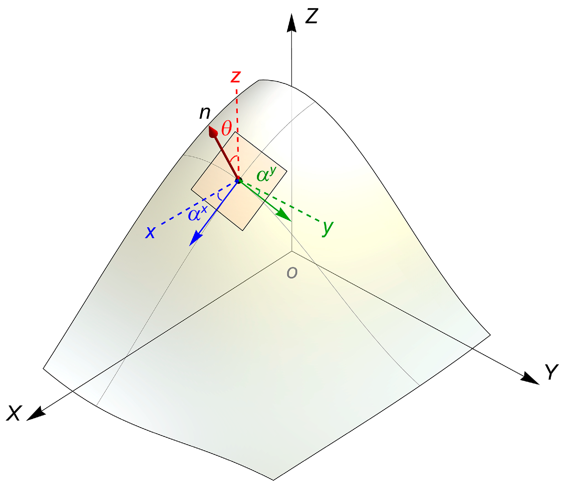
2.2. The Depth-Averaged Mass Flow Model for Diffusive Rock Avalanche

In the later stage of the landslide, the sliding mass is usually broken and disintegrated into smaller blocks in the friction and collision process with the basal bed. Landslides usually exhibit obvious diffusive and high mobility characteristics. Therefore, the depth-averaged models based on the principles of hydrodynamics or particle dynamics are more suitable. Depth-averaged dynamic models have been widely used in the analysis of landslide or debris flow events with high mobility [2,43,44]. When analyzing landslides with the Global Cartesian System (GCS) under steep terrain, the gravitational acceleration should be corrected [45,46].

When the depth-averaged model is applied to the GIS system, the correction based on the terrain slope in the Global Cartesian System (GCS) is more convenient. In this case, the component of gravitational acceleration in the direction perpendicular to the basal bed can be expressed as

$$\mathbf{g}·\mathbf{n}=g\mathrm{c}\mathrm{o}\mathrm{s}\theta =\frac{g}{\sqrt{(\partial z_b/\partial x{)}^2+(\partial z_b/\partial y{)}^2+1}},$$

(18)

Following the work of García-Navarro [47] on the non-erosive depth-averaged model under GCS and the theory of Pudasaini [36] about the erosional landslide, the depth-averaged model of erosive granular flows under GCS can be expressed as

$$\left\{\begin{array}{c}\frac{\partial h}{\partial t}+\frac{\partial }{\partial x}\left(hu\right)+\frac{\partial }{\partial y}\left(hv\right)=E\\ \frac{\partial }{\partial t}\left(hu\right)+\frac{\partial }{\partial x}(h{u}^2+\frac{K_x}{2}{g}_{\theta }{h}^2)+\frac{\partial }{\partial y}\left(huv\right)=-g_{\theta }h\frac{\partial z_b}{\partial x}-\frac{\tau }{\rho }\frac{s_x}{\mathrm{c}\mathrm{o}\mathrm{s}\theta }+2{\lambda }_{b}uE\\ \frac{\partial }{\partial t}\left(hv\right)+\frac{\partial }{\partial x}\left(huv\right)+\frac{\partial }{\partial y}(h{v}^2+\frac{K_y}{2}{g}_{\theta }{h}^2)=-g_{\theta }h\frac{\partial z_b}{\partial y}-\frac{\tau }{\rho }\frac{s_y}{\mathrm{c}\mathrm{o}\mathrm{s}\theta }+2{\lambda }_{b}vE\\ \frac{\partial Z_b}{\partial t}=-E\end{array}\right.$$

(19)

where the first equation represents the conservation of mass, the second and third equations represent the conservation of momentum in the x and y directions, respectively, and the fourth equation represents the evolution of the bed elevation due to erosion.

Equation (19) can also be expressed in a compact form as

$$\frac{\partial \mathbf{U}}{\partial t}+\frac{\partial \mathbf{F}\left(\mathbf{U}\right)}{\partial x}+\frac{\partial \mathbf{G}\left(\mathbf{U}\right)}{\partial y}=\mathbf{S}={\mathbf{S}}_b+{\mathbf{S}}_{\tau }+{\mathbf{S}}_E,$$

(20)

where the vector of conservation variables is U = (h, hu, hv, z_b)^T, with h representing the flow depth in the vertical z coordinate (Figure 2), and (u, v) are the depth-averaged velocity components along the x, y directions, respectively.

The vector of flux in the x and y directions is denoted by F and G, respectively. Under global Cartesian coordinates, on the erodible bed, these fluxes are given by

$$\mathbf{F}(\mathbf{U})={(hu,h{u}^2+\frac{1}{2}{K}_x{g}_{\theta }{h}^2,huv,0)}^{\mathrm{T}},$$

(21)

$$\mathbf{G}(\mathbf{U})=(hv,huv,h{v}^2+\frac{1}{2}{K}_y{g}_{\theta }{h}^2,0{)}^{\mathrm{T}},$$

(22)

where the lateral pressure coefficients in the x and y directions are denoted as K_x and K_y, respectively (refer to [26]).

The corrected acceleration of gravity ${\mathrm{g}}_{\mathsf{\theta }}=\mathrm{g}{\cos }^2\mathsf{\theta }$ takes into account the influence of steep terrain in global coordinates [45]. The variable θ represents the angle between the normal of the bed and the vertical coordinate axis (see Figure 2).

The source terms on the right hand of Equation (20) are given by

$${\mathbf{S}}_b=(0,-g_{\theta }h\frac{\partial z_b}{\partial x},-g_{\theta }h\frac{\partial z_b}{\partial y},0{)}^{\mathrm{T}},$$

(23)

$${\mathbf{S}}_{\tau }={(0,-\frac{{\tau }_b}{\rho }\frac{u}{\parallel \mathbf{u}\parallel },-\frac{{\tau }_b}{\rho }\frac{\nu }{\parallel \mathbf{u}\parallel },0)}^{\mathrm{T}},$$

(24)

$${\mathbf{S}}_E={(E,2{\lambda }_{b}uE,2{\lambda }_{b}vE,-E)}^{\mathrm{T}},$$

(25)

where S_b, S_τ, and S_E represent the source term of topography, basal friction, and entrainment, respectively.

Regarding the basal friction source term, the classical Voellmy–Salm friction law can be used, which is given by

$$\frac{{\tau }_b}{\rho }=\frac{{\tau }_c}{\rho }+g\frac{{\parallel \mathbf{u}\parallel }^2}{\xi }=\mu gh{\mathrm{c}\mathrm{o}\mathrm{s}}^2\theta +\frac{g(u^2+v^2+w^2)}{\xi },$$

(26)

where the variables μ and ξ represent the dry Coulomb friction coefficient and velocity-dependent viscous or turbulent friction coefficient, respectively. In addition to the friction force, a viscous force should be considered in some cases. This additional viscous force approximates the energy dissipation effects caused by the plastic strain and collision of the rock mass during sliding. This viscous force has also been adopted in similar studies [48,49,50].

The introduction of entrainment causes changes in the mass and momentum conservation equations [36,46]. According to Equation (19), due to the entrainment, the change in bed elevation is

$$\frac{\partial z_b}{\partial t}=-E,$$

(27)

where E = E (x, y, t) is the mass production source term, which represents the entrainment rate (E > 0) or deposition rate (E < 0). The detailed variation characteristics are determined by the entrainment rate formula represented by E, which will be discussed in the following section.

2.3. Entrainment Rate and Corresponding Production Source Terms

Experiments and field observations have shown that erosion and subsequent entrainment can significantly alter the dynamic characteristics of geophysical mass flow [27,51,52]. During the entrainment process, part of the eroded material along the path will be accelerated and entrained into the avalanche. During this process, mass and momentum exchange between the avalanching body and the bed. The dynamic model represented by Equation (19) contains mass and momentum production (in terms of entrainment rate) caused by mass entrainment. The entrainment rate describes the quantity of mass that is entrained into (or detached from) the avalanching body per unit of time. Various entrainment rate formulas have been proposed for special types of avalanche events (e.g., [46,53,54]).

An empirical entrainment model [55] will be used in this study, in which the entrainment rate E is determined by multiplying an empirical coefficient C_E with the bulk momentum M of the flow:

$$E={\mathrm{C}}_{\mathrm{E}}\mathrm{M}$$

(28)

where the empirical coefficient C_E is usually determined concerning similar practical applications [56,57].

Since the entrainment rate represents the mass amount added to or removed from the flow per unit of time, it can be directly introduced into the mass conservation equation. The entrainment-induced momentum should be introduced into the momentum conservation equation based on rigorous physical principles. When erosion occurs, the eroded species on one side of the eroded interface often do not directly gain the same velocity as the flow on the other side of the eroded interface [46,54]. The variable λ_b in Equation (25) is the erosion drift coefficient that connects the mean flow velocity u of a landslide to the velocity of the eroded mass, u_b = λ_bu. Pudasaini and Krautblatter [36] derived a full set of dynamic equations in which the erosion-induced change in inertia and the net momentum production (i.e., 2λ_bEu) have been included in the momentum balance equations. Following their work, the same entrainment source terms were used in Equation (25). Entrainment is treated as a complementary function in r.avaflow, which will be executed at the end of each time step in a forward Euler manner. The complementary functions can be considered a reasonable first approximation of the entrainment [55].

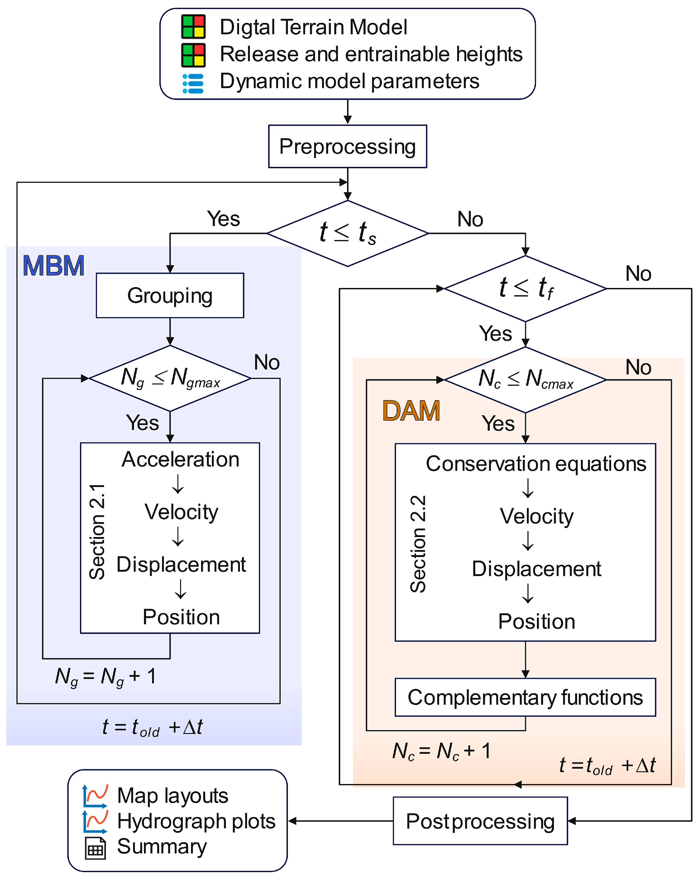
2.4. Workflow of the Integrated Dynamic Model

To consider the transition of the landslide from progressive sliding to fast avalanche, the previously introduced multi-block model and depth-averaged model should be effectively integrated into the time sequence [32]. In both models, the blocks represented by the cells have two velocity components. In the multi-block model, each block within a group has the same velocity component, which is the average velocity component of the group. The two models share the same basic variables; therefore, they can be directly integrated. The accuracy of physical quantities within a group is not determined by the spatial dimension of the group but by the basic cells that make up the group. Since the size of the cell remains constant, grouping will not reduce the precision of the physical quantity.

To integrate multi-block and depth-averaged models, a critical time at which model switching occurs should be determined based on the fracture mechanism or field conditions. Aaron and Hungr [32] suggest that this parameter can be determined based on an examination of the pre-sliding topography to identify topographic obstacles or sudden changes in slope that may cause the fragment. The execution process of the integrated model is shown in Figure 3, where t_s is the critical time corresponding to the transition time of the movement state, and t_f is the total time length of the simulation that is specified by the user. MBM means multi-block model, and DAM means depth-averaged model. N_gmax and N_cmax are the total number of groups and cells, respectively. At present, the determination of the critical time t_s for switching from MBM to DAM can mainly be based on the characteristics of the terrain. Some specific terrain or obstacles are often prone to fragmentation, such as obvious protrusions on the terrain or highways. Based on the distance between these terrains and the landslide source area, combined with the estimated landslide initiation speed, the critical time value can be estimated. In the back-analysis of landslides, this time can be adjusted after simulations to make the simulation results more consistent with the site.

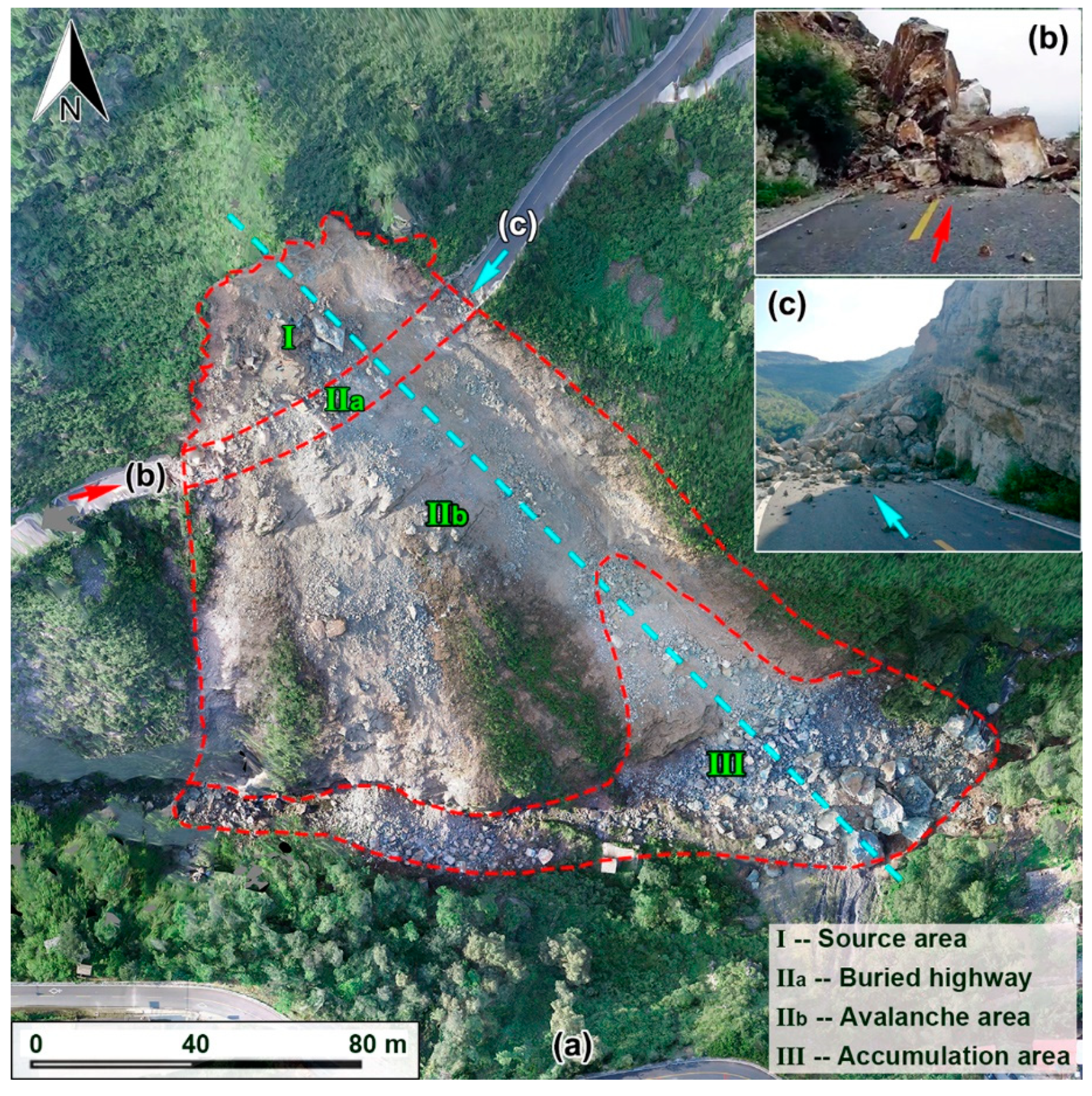
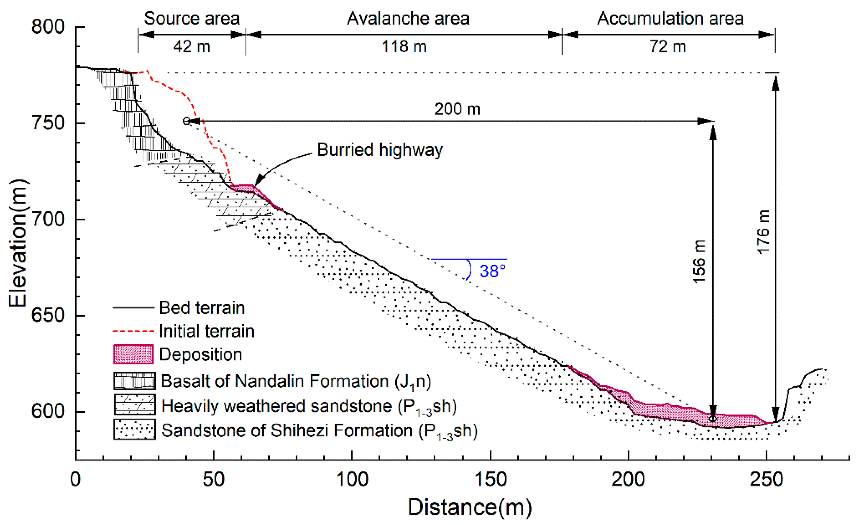
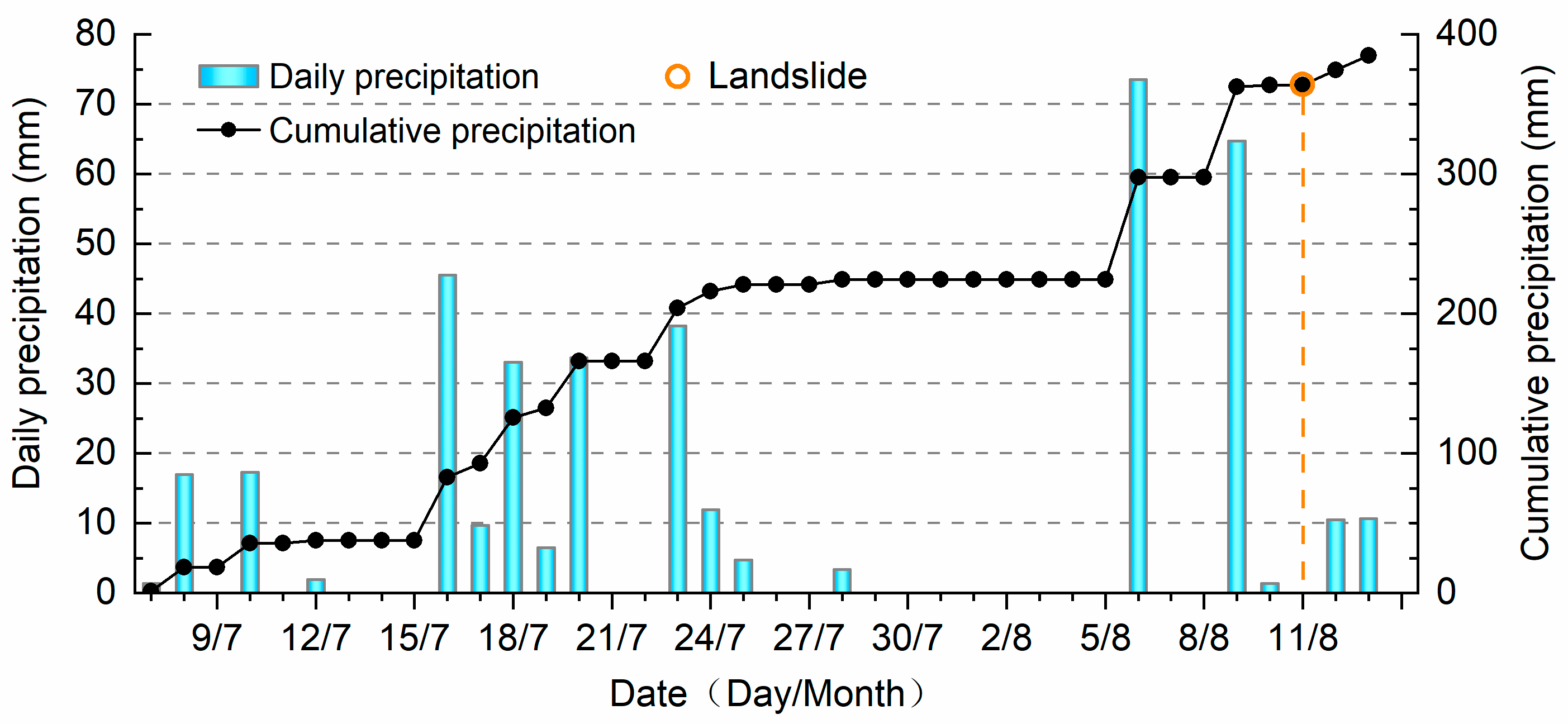
3. Overview of the Da’anshan Landslide Disaster

A rockslide–debris avalanche occurred on 11 August 2018, in the Da’anshan village, Fangshan district of Beijing, China (115°45′49.37″ E, 39°53′14.67″ N). The rock mass collapsed from the head scarp of the slope and impacted the Junhong Highway below the source area. The Junhong Highway is one of the important highways in the Fangshan District, with a total length of 19.8 km and a road width of 7 m. The violent impact of the rock against the road resulted in severe disaggregation, and the fragmented rock slid down the slope diffusively. Severely weathered rocks and vegetation on the slope were eroded and entrained by the avalanche. The slowly triggered rockslide turned into a rapid debris avalanche. The affected region can be roughly divided into three areas, namely the source area, the avalanche area, and the accumulation area (Figure 4a). The red dashed line outlines the boundaries of different zones; the cyan dashed line represents a vertical profile section, along which data will be extracted in the subsequent simulations. A road with a section width of about 80 m was blocked by the collapsed gravel rocks (Figure 4b,c). By comparing the digital elevation maps before and after the landslide, the mobilized rock in the source area can be estimated to be 3.1 × 10⁴ m³. The height difference between the front edge of the accumulation area and the rear edge of the source area is about 176 m. Correspondingly, the sliding mass traveled a maximum horizontal distance of about 232 m (Figure 5).

The digital elevation data, which were extracted along one of the main avalanche paths (the cyan dotted line in Figure 4a), were plotted in Figure 5. The angle between the north and this avalanche path is approximately 134.7° clockwise. In Figure 5, the ratio of height loss to the traveled distance of the landslide mass center is about 0.78. The maximum horizontal avalanche distance (L_max) is about 232 m, the maximum height difference (H_max) is about 176 m, and the H_max/L_max ≈ 0.82; this ratio is also relatively high for a rock landslide. These ratios reflect that the avalanche distance of this landslide is much smaller than that of a normal landslide. This landslide destabilized gradually and collided with the road below it; kinetic energy was consumed during this process.

Da’anshan Township is in the northwest of Fangshan District, covering an area of 62.29 km², including about 45 km² of forest land. Da’anshan Township has complex terrain and landforms, and the maximum relative elevation difference is about 1371 m. The Da’anshan landslide body is mainly composed of moderately and strongly weathered metamorphic basalt of the Jurassic Nandaling Formation with well-developed columnar joints and gray-white gravelly quartz sandstone of the Permian Shihezi Formation (Figure 5). The slope near the highway contains soft–hard interlayered rock (Figure 6a). Field measurements show that there are mainly three to five groups of obvious structural planes. Local rock masses have a relatively high degree of fragmentation (Figure 6b). The widely distributed fissures in the rock mass cause the water infiltrated by rainfall to seep out of the local surface of the rock mass. Under the influence of recent rainfall infiltration, water seeps from the rock fissures at the foot of the slope (Figure 6c).

The Da’anshan area is in a sub-humid, warm-temperature continental monsoon climate zone. It has an average annual temperature of 10–12 °C and abundant rainfall in the summer. Meteorological data from the observation point in Da’anshan Village showed that the cumulative daily rainfall from 7 July to 10 August (the day just before the landslide) had reached 364 mm (Figure 7). The daily rainfall exceeded 70 mm and 60 mm on August 6 and 9, respectively. The infiltration of rainfall will lead to an increase in pore pressure, and the long-term immersion of water will lead to the decline in rock strength, especially in the shatter zone of the slope. The landslide occurred after two heavy rainfall events in August, so the recent heavy rainfall was one of the main factors triggering the landslide.

Screenshots in Figure 8 are from the video recorded by the witness. The numbers marked in the upper-right corner of each image represent the time in “seconds: milliseconds” format. For the convenience of comparison, we regard the time when the slope toe showed visible deformation in the video as the initial time (marked as 0:000 in the upper-right corner of Figure 8a). The instability of the slope first occurred at the foot of the slope, near the pavement of the road (marked with a yellow dotted line).

At 1 s (Figure 8b), the top of the unstable slope was partially detached from the surrounding stable slope. After that, the range of detachment expanded laterally, but the downward displacement at the top developed slowly. At 1 s 952 ms (Figure 8d), the displacement has become obvious, but the displacement at the lower part of the slope (near the yellow dotted line) is still small, and the soil protruding downward from this part has not reached the pavement. The sliding body maintained good integrity during this process. At 2 s 952 ms (Figure 8e), the downward displacement of the top of the landslide is further increased, and a small number of broken stones near the slope foot fall onto the pavement and stir up dust. At 3 s 952 ms (Figure 8f), the sliding body decomposes significantly during the impaction process with the road surface. With the development of displacement, the integrity of the landslide declined, and the main part of the landslide hit the pavement and aroused a lot of dust (Figure 8g,h). Thereafter, both the impact area and avalanche velocity of the landslide increased significantly. Then, the rockslide gradually evolved into a rock avalanche.

4. Numerical Modeling of Da’anshan Landslide

4.1. Numerical Tool for Landslide Modeling

Numerical modeling is an applicable method for analyzing complex geophysical mass flows and offers an effective tool for exploring disaster mechanisms via inverse analysis [44,57] or parameter sensitivity analysis [3,58,59]. Some numerical tools have been widely applied in geological hazard analysis, such as r.avaflow [55,57,59,60], D-Claw [2,12,60,61], TITAN2D [62], DAN (DAN3D) [17,52,63,64], and Massflow [31,65].

DAN3D [64] is a Lagrangian implementation of the depth-averaged model with equivalent fluid assumption. DAN3D was derived in a Lagrangian coordinate system, with the x- and y-coordinate located in the plane tangent to the terrain and the z-coordinate oriented in the bed-normal direction [27]. Therefore, before numerical simulation, it is necessary to convert the digital elevation model in the global coordinate system into the digital terrain in the Lagrangian coordinate system mentioned above. DAN3D has achieved the integration of two different dynamic models and has been applied to the analysis of disasters [27,32]. The other numerical tools mentioned above are mainly depth-averaged dynamic models and have not yet been integrated with other models such as the sliding block model [18] and the mass point method (lumped mass model) [14,15].

The numerical tool r.avaflow “http://avaflow.org (accessed on 8 October 2022)” was designed as a plug-in based on open-source GIS software (GRASS GIS V7.8). It utilizes C language to execute core compute modules and the R and Python languages for auxiliary tasks such as data transfer and post-processing of results. The V2.4 pre-release version of r.avaflow includes a mixture flow (single-phase) model and a multiphase flow model [25]. Several enhancements have been implemented within this version, including an enhanced drag force module [66] and virtual mass force formulation [67]. As open-source software, the functions of r.avaflow can be easily customized or extended. The versatility of r.avaflow has been verified in various disaster events [43,44,56,57,59,68,69].

In this study, the numerical tool r.avaflow was utilized, which provides a computational framework based on the total-variation-diminishing (TVD) non-oscillatory central differencing (NOC) scheme [70]. For modeling the Da’anshan rockslide–debris avalanche event, a customized model that integrates the multi-block model (Section 2.1) and the depth-averaged model (Section 2.2) was implemented in r.avaflow. The influence of bed entrainment effects was also considered (Section 2.3). The advantages of this integrated model will be discussed. In this study, all the numerical simulations and the output results were carried out with the help of GRASS GIS.

4.2. Inputs and Parameters for Simulations

Digital elevation maps (DEMs) before and after the landslide are needed in the simulations. By comparing the elevation difference between these two DEMs, the extent and height of the mobilized mass in the source area were determined. The pre-sliding digital terrain was reconstructed using an 8 m resolution DEM, combined with high-resolution remote sensing images two months before the landslide. The same method was used to obtain the digital terrain after the landslide, which occurred a few days after the landslide occurred. The digital elevation maps used in the current analysis have a final resolution of 2 m.

The bulk density ρ, internal friction angle φ, and basal friction angle δ are determined based on the empirical values in similar landslide analyses. These values remain constant in both dynamic models. The turbulent coefficient is needed only in the depth-averaged model. Referring to similar landslide simulations [44,59] and via trial calculation, the entrainment coefficient is taken as 10^−6.2 in this study. For the sliding block model, the size of the block is 6 m, which means nine blocks form one group (see Figure 1). The size of the group needs to be determined via on-site investigation combined with the distribution of rock joints and the degree of weathering. The values of some parameters have referred to similar landslide analyses and the actual geological conditions of this landslide. Special parameters, such as cohesive stress, are determined via trial calculations. The model parameters and corresponding values are summarized in

Table 1. Main model parameters used in the simulations.

Symbol	Parameter	Unit	Value
ρ	Bulk density	Kg/m3	2500
φ	Internal friction angle	Degree	38
δ	Basal friction angle	Degree	30
c	Cohesion stress	KPa	10
ξ	Turbulent coefficient	m/s2	600
CE	Entrainment coefficient	-	10–6.2

.

4.3. Numerical Simulation Results and Analysis

To analyze the influence of early sliding duration t_s on the dynamic characteristics of landslides, three numerical simulations with different t_s were carried out. The t_s of simulation (Ⅰ) is 4 s, which is the closest to the sliding time obtained from the video recording. In simulation (Ⅰ), within the initial 4 s, the dynamic characteristics of the landslide are simulated with the multi-block model. After that, the landslide dynamic characteristics are controlled by the depth-averaged dynamic model.

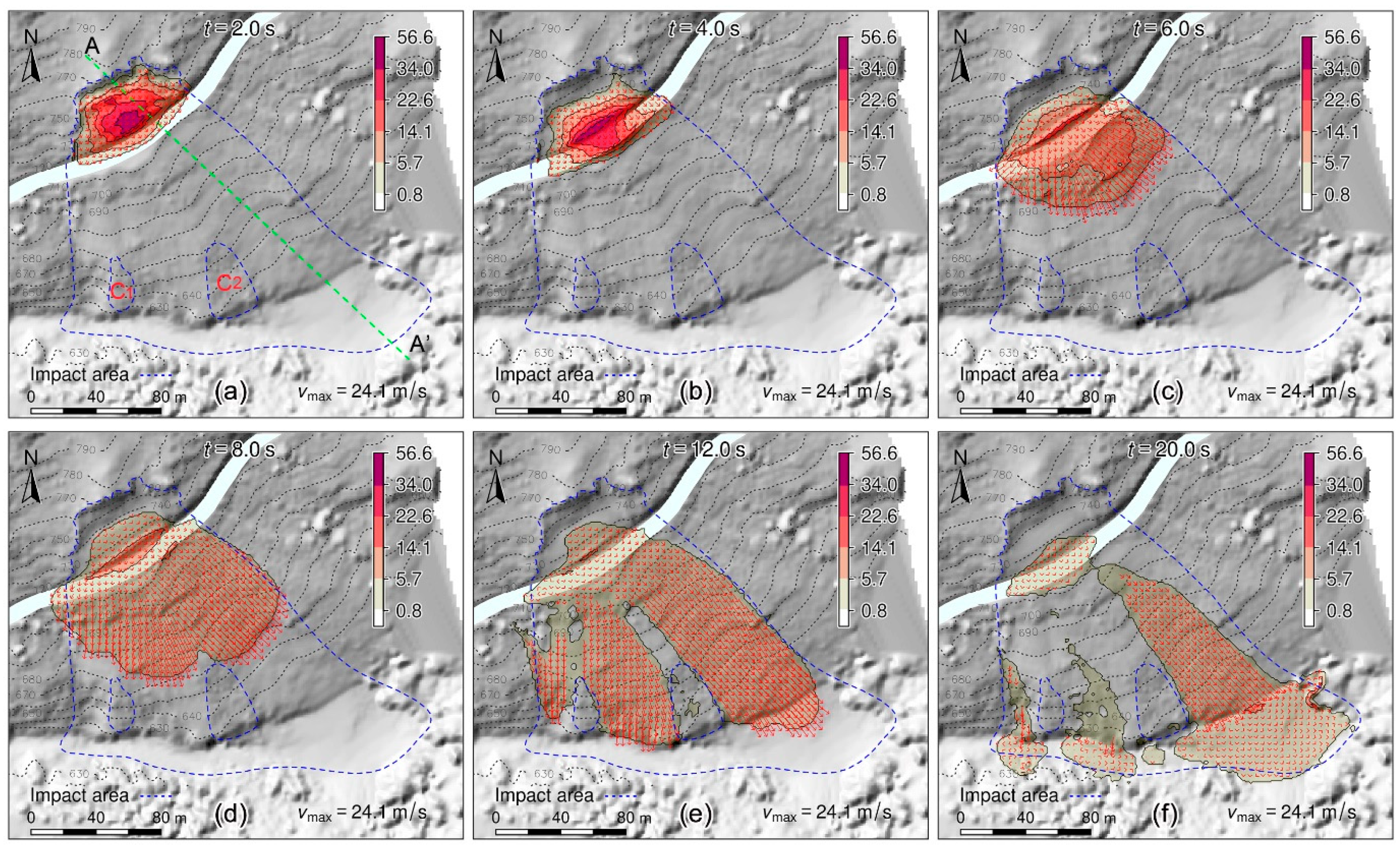
4.3.1. Flow Height Characters of Simulation (Ⅰ)

The distributions of the simulated flow heights at different times are presented in Figure 9 (The blue dashed line represents the extent of the avalanche impact area; the green dashed lines represent the profile line used for flow height extraction in Figure 4a; and C1 and C2 mark two locally convex terrains). At 2.0 s (Figure 9a), the detached rock mass slides down a very short distance, and the sliding body almost maintains its original shape. The front of the landslide has slid onto the pavement. At 4.0 s (Figure 9b), the landslide continued to slide downhill. The coverage area of the landslide did not clearly change, and the front of the landslide slid across the pavement and moved a very small distance in the downhill direction. The position of the landslide front is consistent with the image extracted from the video (Figure 8f). After 4.0 s, the dynamics of the landslide are controlled by the depth-averaged model introduced in Section 2.2. At 6.0 s (Figure 9c), the impacted area of the avalanche body spreads out significantly. By comparing the magnitude of the velocity represented by the arrow line length in Figure 9, it can be found that the speed at this time was significantly greater than that before 4 s. This reflects the phenomenon of rapid expansion of the landslide after disintegration (Figure 8g,h). At 8 s (Figure 9d), the landslide continues to spread downhill at a high speed. At 12 s (Figure 9e), the landslide bypasses the locally convex terrain and slides downhill. The front of the landslide reaches the foot of the slope. At 20 s (Figure 9f), almost all unstable soils have runout from the source area, and a pile of soil with a length of about 66 m has remained on the pavement. The impacted area in the flat area at the slope foot is close to the actual final accumulation range (marked by the blue dashed lines in Figure 9). The global maximum avalanching velocity obtained from numerical simulation (Ⅰ) is about 24.1 m/s. The peak velocity of the landslide determined via the analysis of on-site video is 26.1 m/s, which is slightly higher than the numerical simulation results.

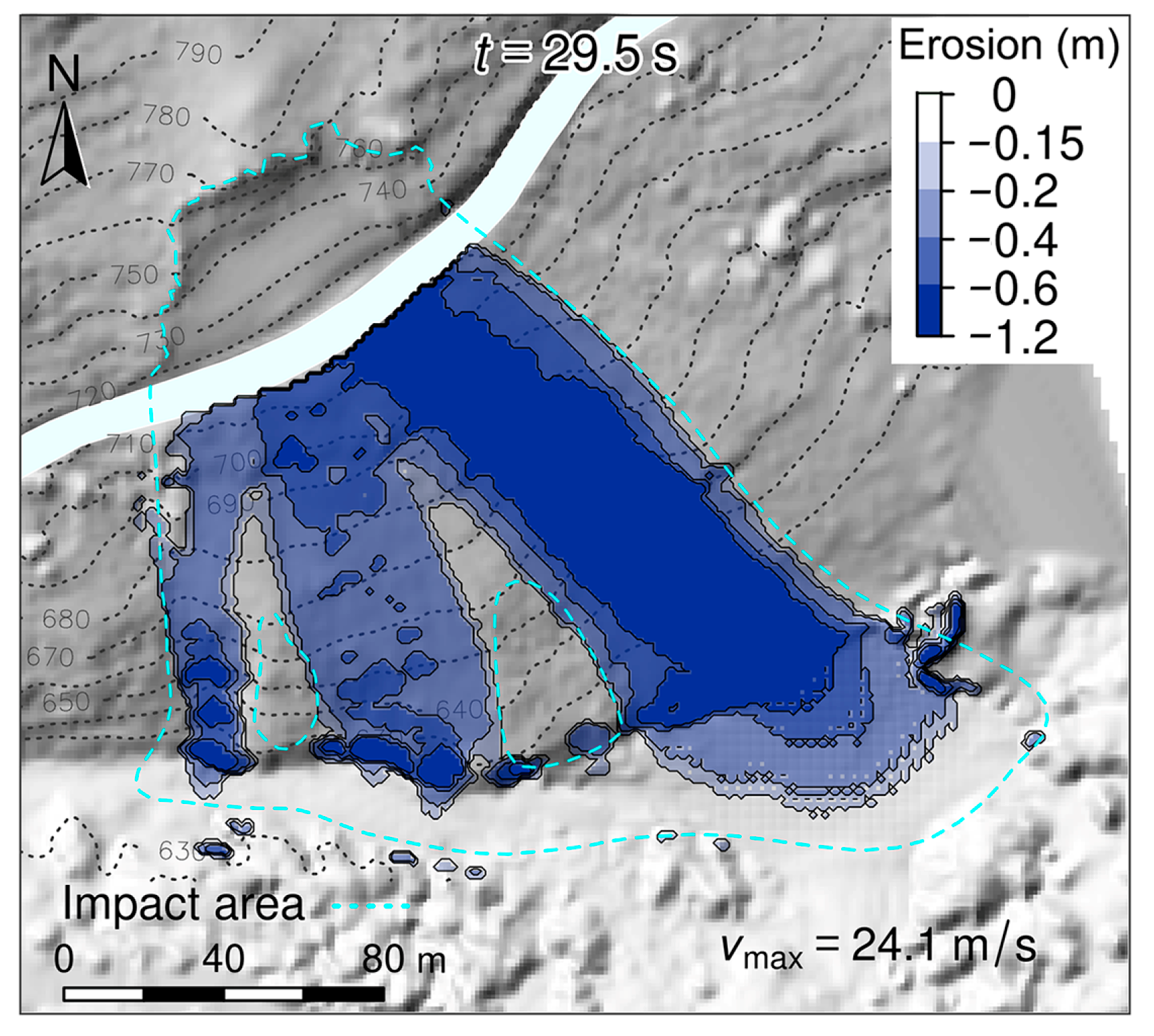
4.3.2. Erosion Character of Simulation (Ⅰ)

The distribution of the simulated erosion depth is shown in Figure 10. The maximum erosion depth mainly occurs in the easternmost of the three sliding paths, which is consistent with the field survey. The maximum erosion depth is about 1.2 m, which is consistent with the field.

4.3.3. Comparison of Flow Depth Characteristics in Different Simulations

To analyze the effect of rigid-like sliding duration (t_s) on the dynamic characteristics of the landslide, two additional simulations with different t_s were carried out. Except for the sliding duration (t_s), all other parameters have the same values in all simulations. For simulation (Ⅱ) and (Ⅲ), t_s = 2 s and 6 s, respectively.

The initial area of the source zone is about 4175 m², and the different evolutions of the simulated impact areas are shown in Figure 11. The impact areas of simulation (Ⅱ), (Ⅰ), and (Ⅲ) increased to 4625 m², 4693 m², and 5367 m²_, respectively in 2 s, 4 s, and 6 s, which increased by 10.8%, 12.4%, and 28.6% relative to the initial area. Therefore, the impact areas increase slowly during the period of the multi-block model. The maximum impact areas for t_s = 2 s, 4 s, and 6 s are 14,399 m², 13,961 m², and 13,415 m², respectively. Within a few seconds of the triggering stage, if the occurrence of disintegration is advanced by 2 s, the maximum impact area will increase by about 3.1% to 4.1%. It can be seen that the smaller the t_s value, the greater the peak value of the impact area. As the block sliding duration (t_s) decreases, the simulation results of the integrated dynamic model should be closer to the single depth-averaged model.

Most depth-averaged models are based on fluid dynamics; these models include the influence of the lateral earth pressure coefficient, which constitutes the diffusion term in the model equations. The larger the lateral earth pressure coefficient, the more obvious the diffusion will be. In a multi-block model, multiple blocks within a group have the same acceleration component, the interaction between blocks is ignored, and there is no lateral diffusion effect between blocks within the group. The greater the spatial extent of a group, the more masses with the same acceleration component are contained within the group. The lower lateral diffusion and the larger group dimension are the main reasons for the low kinetic energy of landslides in the multi-block stage.

In Figure 12, the flow height distributions along the profile line (the green dashed line in Figure 4a and Figure 9a) in three simulations were compared. At 4 s (Figure 12a), simulation (Ⅰ) and (Ⅲ) have the same distribution of flow height because they are both in the multi-block model stage. Only simulation (Ⅱ)experienced a depth-averaged model stage of 2 s; its landslide front edge is about 20 m ahead of the others, and its flow heights are lower than the others. At 6 s (Figure 12b), simulation (Ⅱ) and (Ⅰ)experienced the depth-averaged model stage of 2 s and 4 s, respectively. Therefore, after the outward spreading, the flow height obviously decreased. Since simulation (Ⅲ) was at the end of the multi-block model stage, the height of the flow did not decrease significantly. The gaps between the three landslide fronts further increased.

5. Discussion

It is worth pointing out that in Figure 9a,b, the displacement development of the landslide is very slow, and the deformation is small, which is consistent with the field (Figure 8). Because the integrity of the landslide rock mass is gradually destroyed. However, this motion characteristic is difficult to achieve with depth-averaged models that are based on fluid or particle dynamics [32]. The convection terms have been included in these depth-averaged models, which makes them have obvious diffusivity. Excessive lateral spreading will be observed when the depth-averaged model is applied alone.

The evolution characteristics of landslide total kinetic energy in these three simulations are different, which can be seen in Figure 13.

In simulation (Ⅱ) (t_s = 2 s), the total kinetic energy of the landslide increases slowly in the first 2 s but rapidly after 2 s, corresponding to a steep kinetic energy segment. In simulation (Ⅰ) (t_s = 4 s), about the first 3 s, the total kinetic energy increases slowly; after that, the total kinetic energy decreases until about 4 s, which is mainly due to the interaction between the landslide and the road surface. After 4 s, in the depth-averaged model stage, the total kinetic energy began to increase rapidly. The total kinetic energy of simulation (Ⅲ) also has evolution characteristics similar to those of simulation (Ⅰ). In simulation (Ⅲ), the multi-block model has the longest execution time, and the landslide is affected by the road surface for the longest time, resulting in the largest drop in total kinetic energy in the early stage. Within a few seconds of the triggering stage, if the occurrence of disintegration is advanced by 2 s, the maximum kinetic energy will increase by more than 20%.

Landslides with initial high integrity often gradually disintegrate into fluid-like flows after maintaining a rigid or semi-rigid state for a certain period of time. When using the DAN3D model to simulate a landslide initiated by rainfall, Zhang et al. used two different rheological models, namely Coulomb friction and Voellmy, respectively, in the initiation area and accumulation area [33]. Different rheological models only lead to differences in friction terms. The model is still an equivalent fluid based on the depth-averaged principle, so it is suitable for analyzing landslides with high initial water content and obvious flow characteristics. Aaron et al. integrated the flexible block model with the depth average model of DAN3D and realized the continuation of the two models in time order with the help of liquefaction time parameters [27]. Their simulation results indicate that for landslides with high integrity and internal cohesion strength, the accurate analysis must consider the initial slow movement stage. Because the z-coordinate is vertically upward in the flexible block model but perpendicular to the terrain in DAN3D, a coordinate transformation is needed before the numerical modeling, which may lead to a reduction in calculation accuracy.

6. Conclusions

The dynamic evolution process of landslides may be very complicated due to the deterioration of integrity resulting from fragmentation, erosion, and entrainment along the runout path. These phenomena are common to landslides worldwide and pose great challenges to disaster prediction and early warning. The inverse analysis of typical landslide events can accumulate experience for the adoption of the model and the corresponding parameter values and provide valuable references for the prediction of potential disasters. This study shows that for a gradually triggered landslide with good initial integrity, the model integrating dynamic models with different characteristics can obtain numerical results that are more consistent with the actual disaster, such as avalanche velocity, accumulation range, and erosion characteristics.

When analyzing the gradually triggered landslide, the application of the multi-block model based on a larger group of cells avoids the excessive lateral spreading of the depth average model in the source area, and the results are more consistent with the early movement characteristics of the landslide.

Before the sliding mass undergoes significant fragmentation, the sliding resistance mainly comes from the friction at the bottom, which maintains higher integrity and lower lateral diffusion. Therefore, when the landslide slides in a rigid or nearly rigid state at the initial stage, its kinetic energy increases slowly. Only by fully considering the influence of this process can the simulation results be more consistent with the field.

Although under some special topographic conditions, the final accumulation patterns are not significantly different under different sliding times, their corresponding dynamic evolution processes may be significantly different, such as the evolution of the total kinetic energy of landslides in this study. This obvious difference in total kinetic energy will affect the effectiveness of the disaster prevention and mitigation measures we have adopted. This emphasizes the importance of disaster analysis based on the dynamic process of landslides.

In this study, a method based on terrain conditions was used to estimate the critical time for dynamic feature transformation, which is simple and easy to master. However, methods for determining critical time based on physical principles, such as fracture mechanics and energy principles, are worth further exploration in the future.

References

1. Pudasaini, S.P. A General Two-Phase Debris Flow Model. J. Geophys. Res. 2012, 117, F03010. [Google Scholar] [CrossRef]
2. Iverson, R.M.; George, D.L.; Allstadt, K.; Reid, M.E.; Collins, B.D.; Vallance, J.W.; Schilling, S.P.; Godt, J.W.; Cannon, C.M.; Magirl, C.S.; et al. Landslide Mobility and Hazards: Implications of the 2014 Oso Disaster. Earth Planet. Sci. Lett. 2015, 412, 197–208. [Google Scholar] [CrossRef]
3. McDougall, S. 2014 Canadian Geotechnical Colloquium: Landslide Runout Analysis—Current Practice and Challenges. Can. Geotech. J. 2017, 54, 605–620. [Google Scholar] [CrossRef]
4. Loew, S.; Gschwind, S.; Gischig, V.; Keller-Signer, A.; Valenti, G. Monitoring and Early Warning of the 2012 Preonzo Catastrophic Rockslope Failure. Landslides 2017, 14, 141–154. [Google Scholar] [CrossRef]
5. Willenberg, H.; Eberhardt, E.; Loew, S.; McDougall, S.; Hungr, O. Hazard Assessment and Runout Analysis for an Unstable Rock Slope above an Industrial Site in the Riviera Valley, Switzerland. Landslides 2009, 6, 111–119. [Google Scholar] [CrossRef]
6. Xu, Y.; George, D.L.; Kim, J.; Lu, Z.; Riley, M.; Griffin, T.; De La Fuente, J. Landslide Monitoring and Runout Hazard Assessment by Integrating Multi-Source Remote Sensing and Numerical Models: An Application to the Gold Basin Landslide Complex, Northern Washington. Landslides 2021, 18, 1131–1141. [Google Scholar] [CrossRef]
7. Zeng, P.; Sun, X.; Xu, Q.; Li, T.; Zhang, T. 3D Probabilistic Landslide Run-out Hazard Evaluation for Quantitative Risk Assessment Purposes. Eng. Geol. 2021, 293, 106303. [Google Scholar] [CrossRef]
8. Devoli, G.; De Blasio, F.V.; Elverhøi, A.; Høeg, K. Statistical Analysis of Landslide Events in Central America and Their Run-out Distance. Geotech. Geol. Eng. 2009, 27, 23–42. [Google Scholar] [CrossRef]
9. Corominas, J. The Angle of Reach as a Mobility Index for Small and Large Landslides. Can. Geotech. J. 1996, 33, 260–271. [Google Scholar] [CrossRef]
10. Hunter, G.; Fell, R. Travel Distance Angle for “Rapid” Landslides in Constructed and Natural Soil Slopes. Can. Geotech. J. 2003, 40, 1123–1141. [Google Scholar] [CrossRef]
11. Miao, H.; Wang, G.; Yin, K.; Kamai, T.; Li, Y. Mechanism of the Slow-Moving Landslides in Jurassic Red-Strata in the Three Gorges Reservoir, China. Eng. Geol. 2014, 171, 59–69. [Google Scholar] [CrossRef]
12. Iverson, R.M.; George, D.L. A Depth-Averaged Debris-Flow Model That Includes the Effects of Evolving Dilatancy. I. Physical Basis. Proc. R. Soc. A 2014, 470, 20130819. [Google Scholar] [CrossRef]
13. Bouchut, F.; Fernández-Nieto, E.D.; Mangeney, A.; Narbona-Reina, G. A Two-Phase Two-Layer Model for Fluidized Granular Flows with Dilatancy Effects. J. Fluid Mech. 2016, 801, 166–221. [Google Scholar] [CrossRef]
14. Perla, R.; Cheng, T.T.; McClung, D.M. A Two-Parameter Model of Snow-Avalanche Motion. J. Glaciol. 1980, 26, 197–207. [Google Scholar] [CrossRef]
15. Gassen, W.V.; Cruden, D.M. Momentum Transfer and Friction in the Debris of Rock Avalanches. Can. Geotech. J. 1989, 26, 623–628. [Google Scholar] [CrossRef]
16. Körner, H.J. The Energy-Line Method in the Mechanics of Avalanches. J. Glaciol. 1980, 26, 501–505. [Google Scholar] [CrossRef]
17. Hungr, O. A Model for the Runout Analysis of Rapid Flow Slides, Debris Flows, and Avalanches. Can. Geotech. J. 1995, 32, 610–623. [Google Scholar] [CrossRef]
18. Miao, T.; Liu, Z.; Niu, Y.; Ma, C. A Sliding Block Model for the Runout Prediction of High-Speed Landslides. Can. Geotech. J. 2001, 38, 217–226. [Google Scholar] [CrossRef]
19. Yang, H.Q.; Lan, Y.F.; Lu, L.; Zhou, X.P. A Quasi-Three-Dimensional Spring-Deformable-Block Model for Runout Analysis of Rapid Landslide Motion. Eng. Geol. 2015, 185, 20–32. [Google Scholar] [CrossRef]
20. Savage, S.B.; Hutter, K. The Motion of a Finite Mass of Granular Material down a Rough Incline. J. Fluid Mech. 1989, 199, 177–215. [Google Scholar] [CrossRef]
21. Hutter, K.; Koch, T. Motion of a Granular Avalanche in an Exponentially Curved Chute: Experiments and Theoretical Predictions. Philos. Trans. R. Soc. Lond. Ser. A Phys. Eng. Sci. 1991, 334, 93–138. [Google Scholar] [CrossRef]
22. Pudasaini, S.P.; Eckart, W.; Hutter, K. Gravity-Driven Rapid Shear Flows of Dry Granular Masses in Helically Curved and Twisted Channels. Math. Models Methods Appl. Sci. 2003, 13, 1019–1052. [Google Scholar] [CrossRef]
23. Kelfoun, K. A Two-Layer Depth-Averaged Model for Both the Dilute and the Concentrated Parts of Pyroclastic Currents. J. Geophys. Res. Solid Earth 2017, 122, 4293–4311. [Google Scholar] [CrossRef]
24. Pitman, E.B.; Le, L. A Two-Fluid Model for Avalanche and Debris Flows. Philos. Trans. R. Soc. A Math. Phys. Eng. Sci. 2005, 363, 1573–1601. [Google Scholar] [CrossRef]
25. Pudasaini, S.P.; Mergili, M. A Multi-Phase Mass Flow Model. J. Geophys. Res. Earth Surf. 2019, 124, 2920–2942. [Google Scholar] [CrossRef]
26. Pudasaini, S.P.; Hutter, K. Avalanche Dynamics: Dynamics of Rapid Flows of Dense Granular Avalanches; Springer: Berlin/Heidelberg, Germany, 2007; ISBN 978-3-540-32686-1. [Google Scholar]
27. Aaron, J.; McDougall, S.; Moore, J.R.; Coe, J.A.; Hungr, O. The Role of Initial Coherence and Path Materials in the Dynamics of Three Rock Avalanche Case Histories. Geoenviron. Disasters 2017, 4, 5. [Google Scholar] [CrossRef]
28. Xu, Q.; Fan, X.; Huang, R.; Yin, Y.; Hou, S.; Dong, X.; Tang, M. A Catastrophic Rockslide-Debris Flow in Wulong, Chongqing, China in 2009: Background, Characterization, and Causes. Landslides 2010, 7, 75–87. [Google Scholar] [CrossRef]
29. Dufresne, A.; Geertsema, M. Rock Slide–Debris Avalanches: Flow Transformation and Hummock Formation, Examples from British Columbia. Landslides 2020, 17, 15–32. [Google Scholar] [CrossRef]
30. McDougall, S. A New Continuum Dynamic Model for the Analysis of Extremely Rapid Landslide Motion across Complex 3D Terrain. Ph.D. Dissertation, University of British Columbia, Vancouver, BC, Canada, 2006. [Google Scholar]
31. Zhou, S.; Ouyang, C.; An, H.; Jiang, T.; Xu, Q. Comprehensive Study of the Beijing Daanshan Rockslide Based on Real-Time Videos, Field Investigations, and Numerical Modeling. Landslides 2020, 17, 1217–1231. [Google Scholar] [CrossRef]
32. Aaron, J.; Hungr, O. Dynamic Simulation of the Motion of Partially-Coherent Landslides. Eng. Geol. 2016, 205, 1–11. [Google Scholar] [CrossRef]
33. Zhang, Y.; Xing, A.; Jin, K.; Zhuang, Y.; Bilal, M.; Xu, S.; Zhu, Y. Investigation and Dynamic Analyses of Rockslide-Induced Debris Avalanche in Shuicheng, Guizhou, China. Landslides 2020, 17, 2189–2203. [Google Scholar] [CrossRef]
34. Sassa, K. Geotechnical Model for the Motion of Landslides. In Proceedings of the 5th International Symposium on Landslides, Lausanne, Switzerland, 10–15 July 1988; Volume 1, pp. 37–55. [Google Scholar]
35. Pudasaini, S.P.; Fischer, J.-T. A Mechanical Model for Phase Separation in Debris Flow. Int. J. Multiph. Flow 2020, 129, 103292. [Google Scholar] [CrossRef]
36. Pudasaini, S.P.; Krautblatter, M. The Mechanics of Landslide Mobility with Erosion. Nat. Commun. 2021, 12, 6793. [Google Scholar] [CrossRef] [PubMed]
37. Gregoretti, C.; Stancanelli, L.M.; Bernard, M.; Boreggio, M.; Degetto, M.; Lanzoni, S. Relevance of Erosion Processes When Modelling In-Channel Gravel Debris Flows for Efficient Hazard Assessment. J. Hydrol. 2019, 568, 575–591. [Google Scholar] [CrossRef]
38. Nikooei, M.; Manzari, M.T. Studying Effect of Entrainment on Dynamics of Debris Flows Using Numerical Simulation. Comput. Geosci. 2020, 134, 104337. [Google Scholar] [CrossRef]
39. Aaron, J.; McDougall, S. Rock Avalanche Mobility: The Role of Path Material. Eng. Geol. 2019, 257, 105126. [Google Scholar] [CrossRef]
40. Pal, S.C.; Chowdhuri, I. GIS-Based Spatial Prediction of Landslide Susceptibility Using Frequency Ratio Model of Lachung River Basin, North Sikkim, India. SN Appl. Sci. 2019, 1, 416. [Google Scholar] [CrossRef]
41. Chowdhuri, I.; Pal, S.C.; Janizadeh, S.; Saha, A.; Ahmadi, K.; Chakrabortty, R.; Islam, A.R.M.T.; Roy, P.; Shit, M. Application of Novel Deep Boosting Framework-Based Earthquake Induced Landslide Hazards Prediction Approach in Sikkim Himalaya. Geocarto Int. 2022, 37, 12509–12535. [Google Scholar] [CrossRef]
42. Chen, H.; Lee, C.F. Numerical Simulation of Debris Flows. Can. Geotech. J. 2000, 37, 146–160. [Google Scholar] [CrossRef]
43. Qiao, C.; Ou, G.; Pan, H. Numerical Modelling of the Long Runout Character of 2015 Shenzhen Landslide with a General Two-Phase Mass Flow Model. Bull. Eng. Geol. Environ. 2019, 78, 3281–3294. [Google Scholar] [CrossRef]
44. Mergili, M.; Jaboyedoff, M.; Pullarello, J.; Pudasaini, S.P. Back Calculation of the 2017 Piz Cengalo–Bondo Landslide Cascade with r.Avaflow: What We Can Do and What We Can Learn. Nat. Hazards Earth Syst. Sci. 2020, 20, 505–520. [Google Scholar] [CrossRef]
45. Juez, C.; Murillo, J.; García-Navarro, P. 2D Simulation of Granular Flow over Irregular Steep Slopes Using Global and Local Coordinates. J. Comput. Phys. 2013, 255, 166–204. [Google Scholar] [CrossRef]
46. Iverson, R.M.; Ouyang, C. Entrainment of Bed Material by Earth-Surface Mass Flows: Review and Reformulation of Depth-Integrated Theory. Rev. Geophys. 2015, 53, 27–58. [Google Scholar] [CrossRef]
47. García-Navarro, P. The Shallow Water Equations and Their Application to Realistic Cases. Environ. Fluid Mech. 2019, 19, 1235–1252. [Google Scholar] [CrossRef]
48. Angeli, M.-G.; Gasparetto, P.; Menotti, R.M.; Pasuto, A.; Silvano, S. A Visco-Plastic Model for Slope Analysis Applied to a Mudslide in Cortina d’Ampezzo, Italy. Q. J. Eng. Geol. Hydrogeol. 1996, 29, 233. [Google Scholar] [CrossRef]
49. Corominas, J.; Moya, J.; Ledesma, A.; Lloret, A.; Gili, J.A. Prediction of Ground Displacements and Velocities from Groundwater Level Changes at the Vallcebre Landslide (Eastern Pyrenees, Spain). Landslides 2005, 2, 83–96. [Google Scholar] [CrossRef]
50. Herrera, G.; Fernández-Merodo, J.A.; Mulas, J.; Pastor, M.; Luzi, G.; Monserrat, O. A Landslide Forecasting Model Using Ground Based SAR Data: The Portalet Case Study. Eng. Geol. 2009, 105, 220–230. [Google Scholar] [CrossRef]
51. Hungr, O.; Evans, S.G. Entrainment of Debris in Rock Avalanches: An Analysis of a Long Run-out Mechanism. Geol. Soc. Am. Bull. 2004, 116, 1240. [Google Scholar] [CrossRef]
52. McDougall, S.; Hungr, O. Dynamic Modelling of Entrainment in Rapid Landslides. Can. Geotech. J. 2005, 42, 1437–1448. [Google Scholar] [CrossRef]
53. Gauer, P.; Issler, D. Possible Erosion Mechanisms in Snow Avalanches. Ann. Glaciol. 2004, 38, 384–392. [Google Scholar] [CrossRef]
54. Pudasaini, S.P.; Fischer, J.-T. A Mechanical Erosion Model for Two-Phase Mass Flows. Int. J. Multiph. Flow 2020, 132, 103416. [Google Scholar] [CrossRef]
55. Mergili, M.; Fischer, J.-T.; Krenn, J.; Pudasaini, S.P.R. Avafow v1, an Advanced Open-Source Computational Framework for the Propagation and Interaction of Two-Phase Mass Fows. Geosci. Model Dev. 2017, 17, 553–569. [Google Scholar] [CrossRef]
56. Mergili, M.; Emmer, A.; Juřicová, A.; Cochachin, A.; Fischer, J.-T.; Huggel, C.; Pudasaini, S.P. How Well Can We Simulate Complex Hydro-Geomorphic Process Chains? The 2012 Multi-Lake Outburst Flood in the Santa Cruz Valley (Cordillera Blanca, Perú). Earth Surf. Process. Landf. 2018, 43, 1373–1389. [Google Scholar] [CrossRef]
57. Mergili, M.; Pudasaini, S.P.; Emmer, A.; Fischer, J.-T.; Cochachin, A.; Frey, H. Reconstruction of the 1941 GLOF Process Chain at Lake Palcacocha (Cordillera Blanca, Peru). Hydrol. Earth Syst. Sci. 2020, 24, 93–114. [Google Scholar] [CrossRef]
58. Iverson, R.M.; George, D.L.; Logan, M. Debris Flow Runup on Vertical Barriers and Adverse Slopes. J. Geophys. Res. Earth Surf. 2016, 121, 2333–2357. [Google Scholar] [CrossRef]
59. Mergili, M.; Frank, B.; Fischer, J.-T.; Huggel, C.; Pudasaini, S.P. Computational Experiments on the 1962 and 1970 Landslide Events at Huascarán (Peru) with r.Avaflow: Lessons Learned for Predictive Mass Flow Simulations. Geomorphology 2018, 322, 15–28. [Google Scholar] [CrossRef]
60. Qiao, C.; Ou, G.; Pan, H.; Ouyang, C.; Jia, Y. Long Runout Mechanism of the Shenzhen 2015 Landslide: Insights from a Two-Phase Flow Viewpoint. J. Mt. Sci. 2018, 15, 2247–2265. [Google Scholar] [CrossRef]
61. Iverson, R.M.; George, D.L. Modelling Landslide Liquefaction, Mobility Bifurcation and the Dynamics of the 2014 Oso Disaster. Géotechnique 2016, 66, 175–187. [Google Scholar] [CrossRef]
62. Sheridan, M.F.; Stinton, A.J.; Patra, A.; Pitman, E.B.; Bauer, A.; Nichita, C.C. Evaluating Titan2D Mass-Flow Model Using the 1963 Little Tahoma Peak Avalanches, Mount Rainier, Washington. J. Volcanol. Geotherm. Res. 2005, 139, 89–102. [Google Scholar] [CrossRef]
63. McDougall, S.; Boultbee, N.; Hungr, O.; Stead, D.; Schwab, J.W. The Zymoetz River Landslide, British Columbia, Canada: Description and Dynamic Analysis of a Rock Slide–Debris Flow. Landslides 2006, 3, 195. [Google Scholar] [CrossRef]
64. McDougall, S.; Hungr, O. A Model for the Analysis of Rapid Landslide Motion across Three-Dimensional Terrain. Can. Geotech. J. 2004, 41, 1084–1097. [Google Scholar] [CrossRef]
65. Ouyang, C.; Zhou, K.; Xu, Q.; Yin, J.; Peng, D.; Wang, D.; Li, W. Dynamic Analysis and Numerical Modeling of the 2015 Catastrophic Landslide of the Construction Waste Landfill at Guangming, Shenzhen, China. Landslides 2017, 14, 705–718. [Google Scholar] [CrossRef]
66. Pudasaini, S.P. A Full Description of Generalized Drag in Mixture Mass Flows. Eng. Geol. 2020, 265, 105429. [Google Scholar] [CrossRef]
67. Pudasaini, S.P. A Fully Analytical Model for Virtual Mass Force in Mixture Flows. Int. J. Multiph. Flow 2019, 113, 142–152. [Google Scholar] [CrossRef]
68. Mergili, M.; Fischer, J.-T.; Pudasaini, S.P. Process Chain Modelling with r.Avaflow: Lessons Learned for Multi-Hazard Analysis. In Advancing Culture of Living with Landslides; Mikos, M., Tiwari, B., Yin, Y., Sassa, K., Eds.; Springer International Publishing: Cham, Switzerland, 2017; pp. 565–572. [Google Scholar]
69. Kafle, J.; Kattel, P.; Pokhrel, P.R.; Khattri, K.B. Numerical Experiments on Effect of Topographical Slope Changes in the Dynamics of Landslide Generated Water Waves and Submarine Mass Flows. J. Appl. Fluid Mech. 2021, 14, 861–876. [Google Scholar] [CrossRef]
70. Nessyahu, H.; Tadmor, E. Non-Oscillatory Central Differencing for Hyperbolic Conservation Laws. J. Comput. Phys. 1990, 87, 408–463. [Google Scholar] [CrossRef]
Figure 1. Schematic diagram of landslide. (a) Landslide in physical space; (b) a top view of a group of blocks; (c) a side view of a group of blocks; (d) stresses acting on a typical block.
Applsci 13 12610 g001
Figure 2. A virtual terrain in the global coordinate system (GCS).
Applsci 13 12610 g002
Figure 3. Flow chart of the integrated dynamic model.
Applsci 13 12610 g003
Figure 4. Aerial and on-site photos of the Da’anshan Landslide. (a) Panoramic aerial view and characteristic zoning; (b) large boulders on the west side of the blocked highway; (c) east side of the blocked highway section.
Applsci 13 12610 g004
Figure 5. Engineering geological features of the slope.
Applsci 13 12610 g005
Figure 6. Geological features near the slope toe. (a) The soft–hard interlayer structure (SZ means “Shatter Zone”); (b) strong weathered and shattered zone; (c) fissure water from rock mass.
Applsci 13 12610 g006
Figure 7. The daily and cumulative precipitation in Da’anshan village.
Applsci 13 12610 g007
Figure 8. Video screenshots of the Da’anshan landslide. (a) The triggering moment of landslide, there was no visible detachment on the slope. (b) After 1 s sliding, a small amount of detachment occurred on the slope. (c) After 1 s 476 ms sliding, a small amount of detachment occurred. (d) After 1 s 952 ms sliding, the amount of detachment gradually increased. (e) After 2 s 952 ms sliding, the front of the slide hit the road below it. (f) After 3 s 952 ms sliding, frontal impact range further expanded. (g) After 4 s 476 ms sliding, the front of the landslide slid off the road. (h) After 5 s 476 ms sliding, the main body of the landslide fully fragmented and slid off the road surface.
Applsci 13 12610 g008
Figure 9. Contour plot of the flow heights at different times of simulation (Ⅰ). (a) At t = 2.0 s, the trailing edge of the sliding body has detached from the slope. (b) At t = 4.0 s, the sliding body slid over the road surface. (c) At t = 6.0 s, the sliding mass expands significantly. (d) At t = 8.0 s, the coverage of the landslide further expanded downhill. (e) At t = 12.0 s, the front of the landslide approached the foot of the slope and bypassed two protruding terrains. (f) At t = 20.0 s, the main body of the landslide spread at the foot of the slope. The range covered by the blue dashed line represents the actual impact range of the landslide. The red letters C1 and C2 mark two protruding terrains that have not been impacted by landslides. The green dashed line represents the location of the extracted flow depth in subsequent analysis.
Applsci 13 12610 g009
Figure 10. Distribution characteristics of final erosion depth. The range covered by the cyan dashed line represents the actual impact range of the landslide.
Applsci 13 12610 g010
Figure 11. Comparison of landslide impact areas of three simulations.
Applsci 13 12610 g011
Figure 12. Comparison of flow heights of three simulations.
Applsci 13 12610 g012
Figure 13. Evolutionary characteristics of total kinetic energy in simulations.
Applsci 13 12610 g013