
Estimating RQD for Rock Masses Based on a Comprehensive Approach


Abstract
:1. Introduction
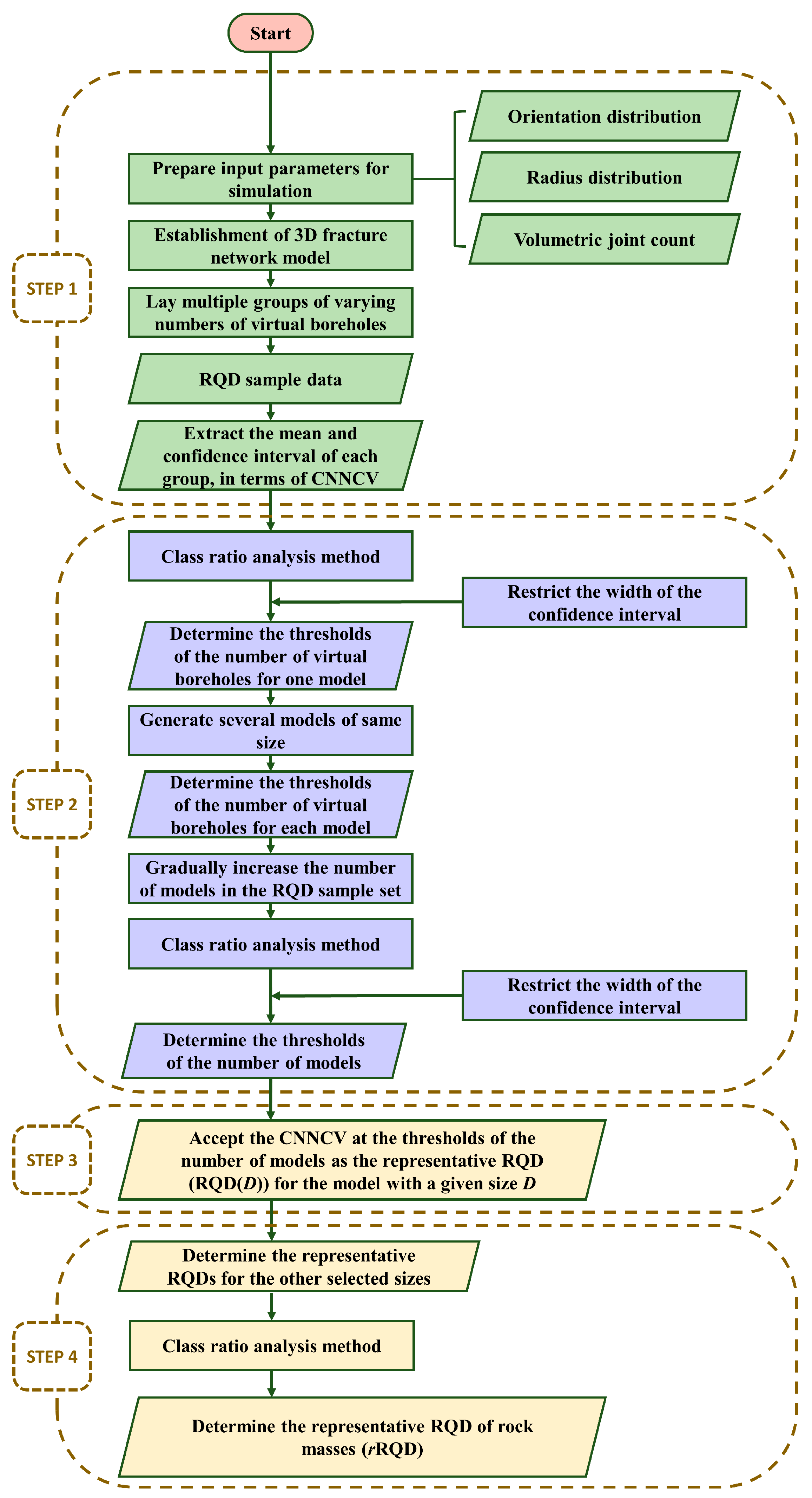
2. The Introduced Approach for Estimating the Representative RQD Based on Class Ratio Analysis
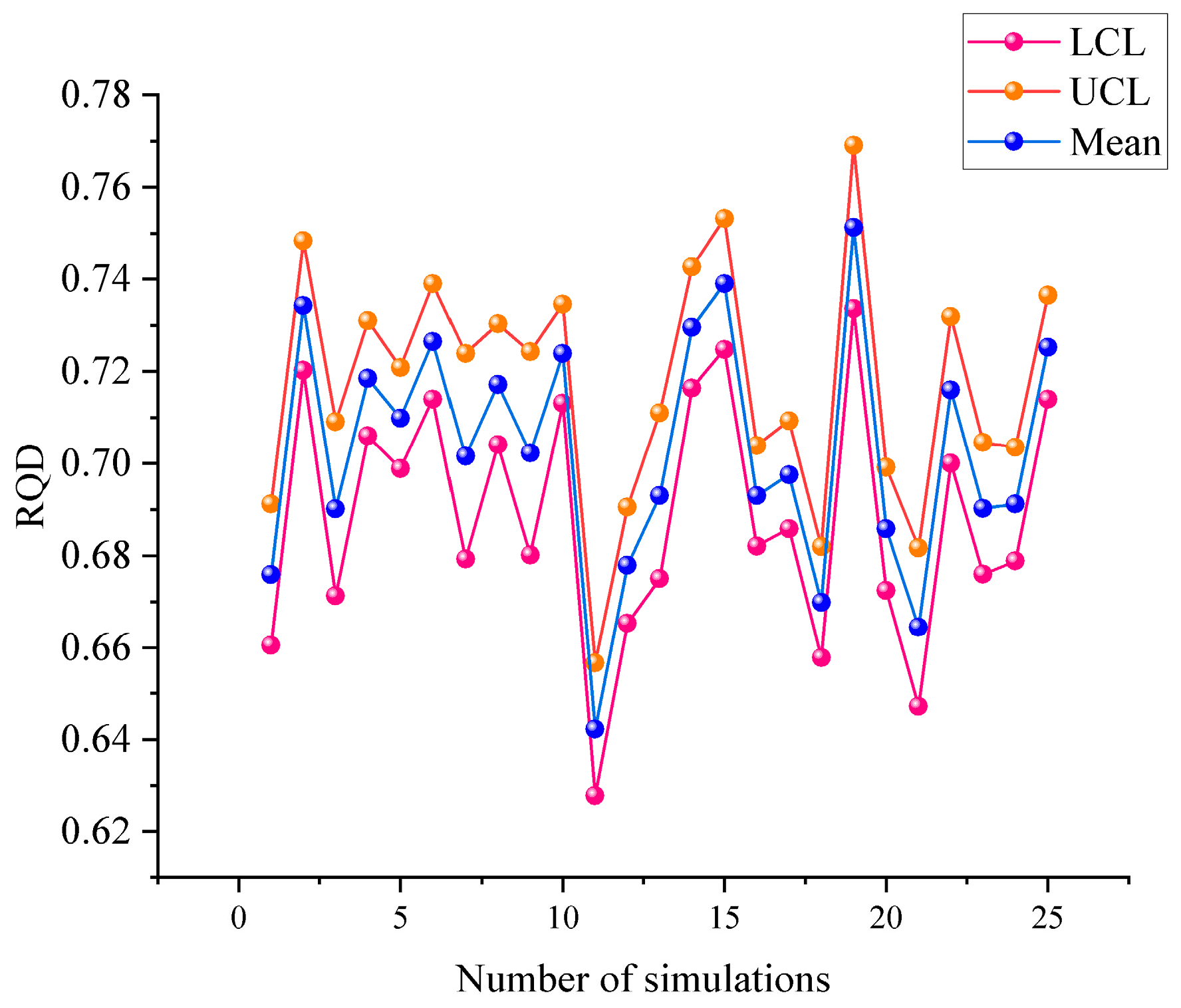
- Extract the mean and confidence interval of the RQD sample, in terms of the Confidence Neutrosophic Number Cubic Value (CNNCV);
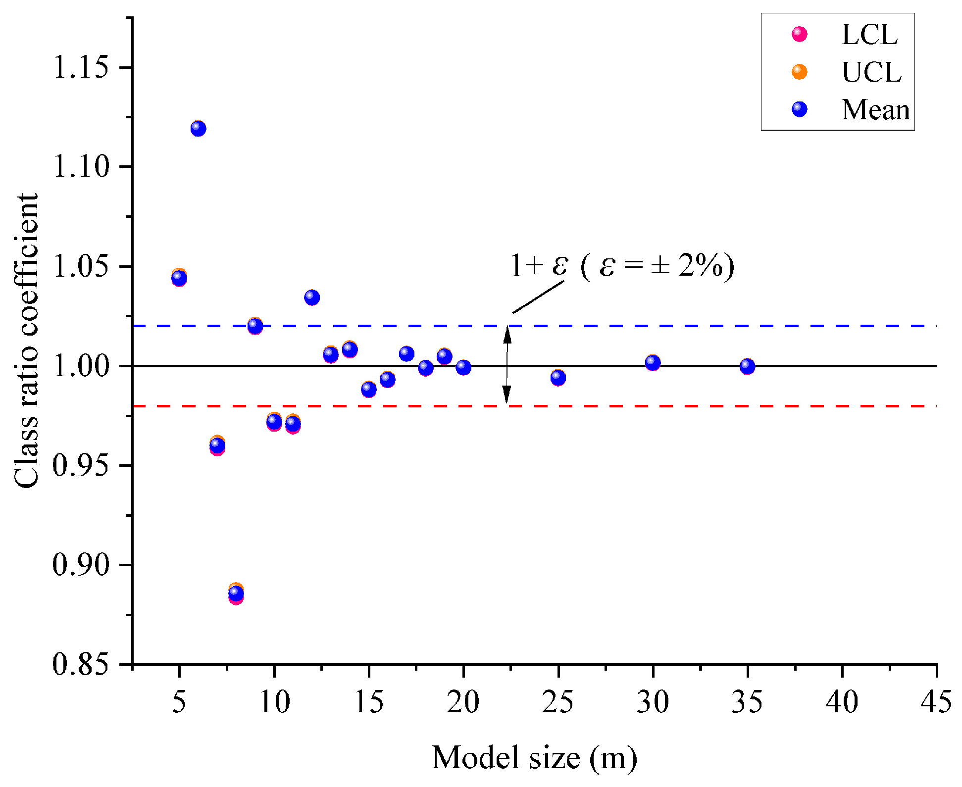
- Employ class ratio analysis to determine the thresholds of the number of virtual boreholes and that of the number of models with a given size D, defined as the specific value which, once exceeded by the number of virtual boreholes and the number of models, the CNNCV does not change significantly;
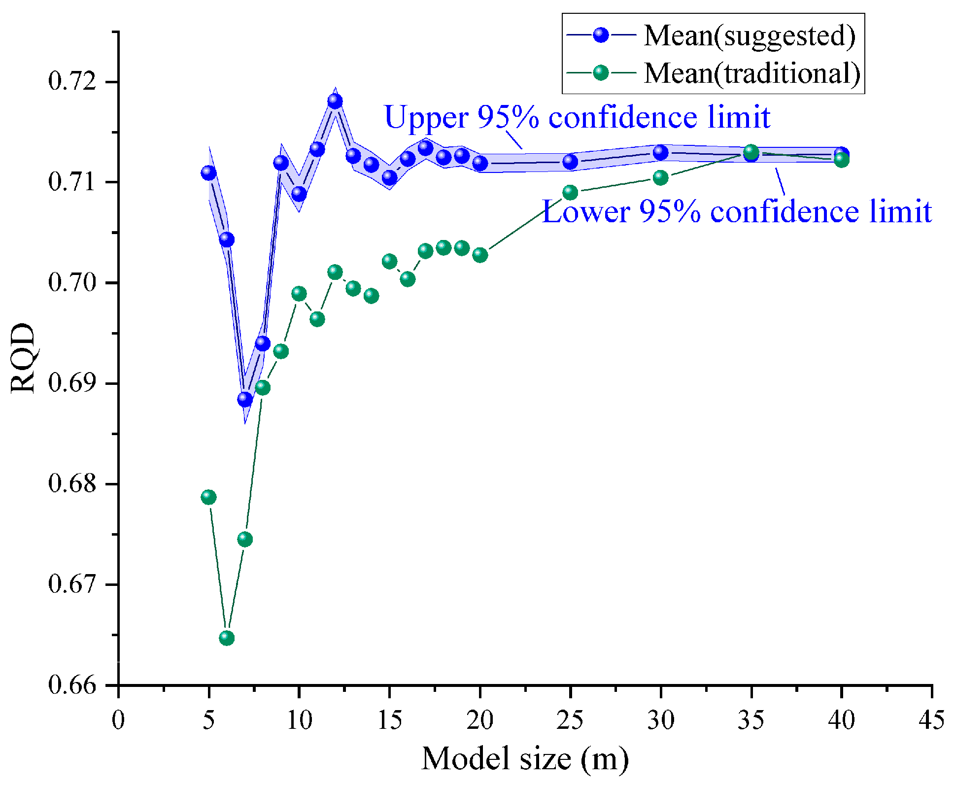
- Accept the CNNCV at the thresholds of the number of models as the representative RQD for the model with a given size D (RQD(D));
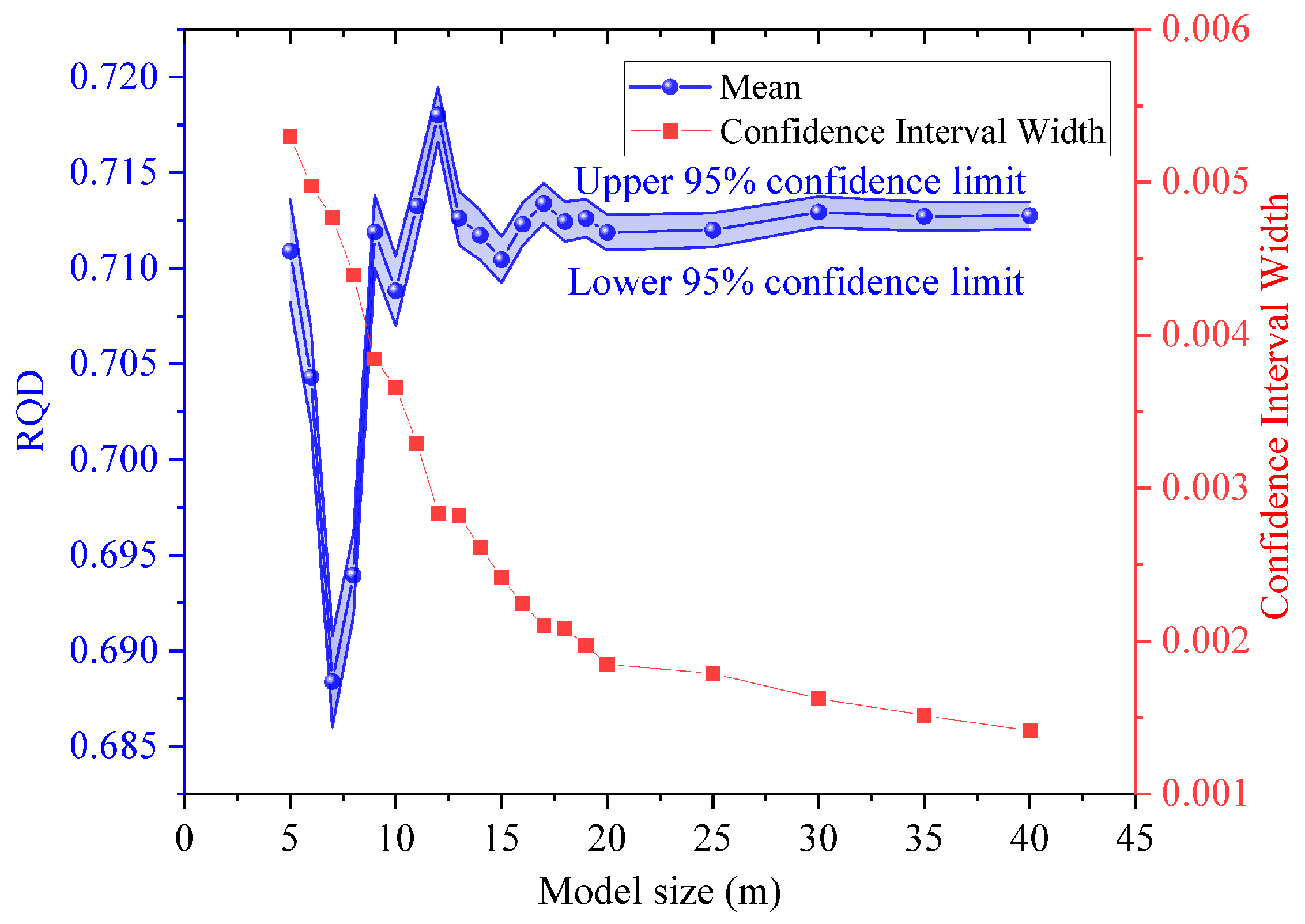
- Determine the representative RQD (rRQD), defined as the specific value which, once D exceeds, the RQD(D) does not change significantly.
2.1. Step 1
2.2. Step 2
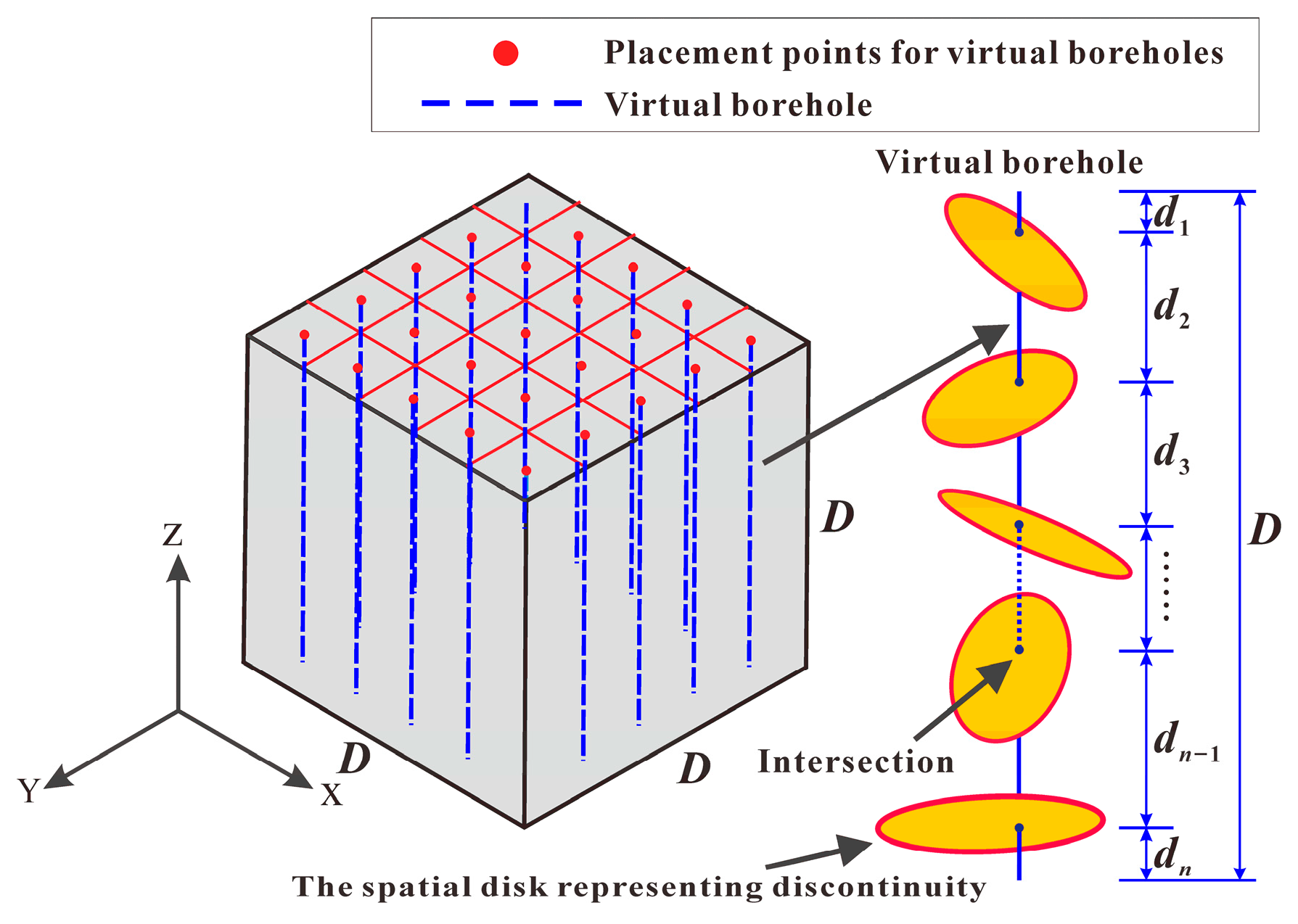
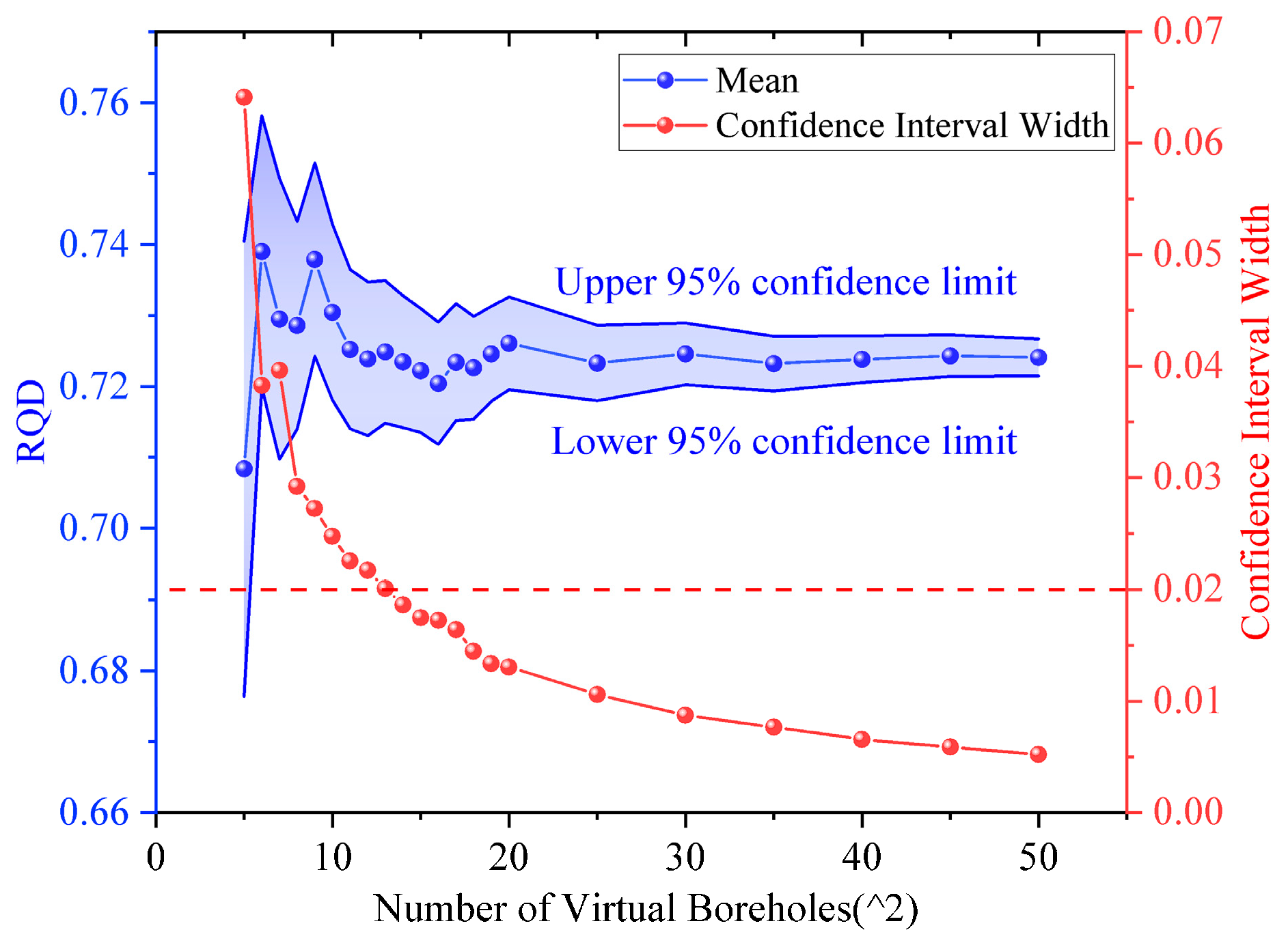
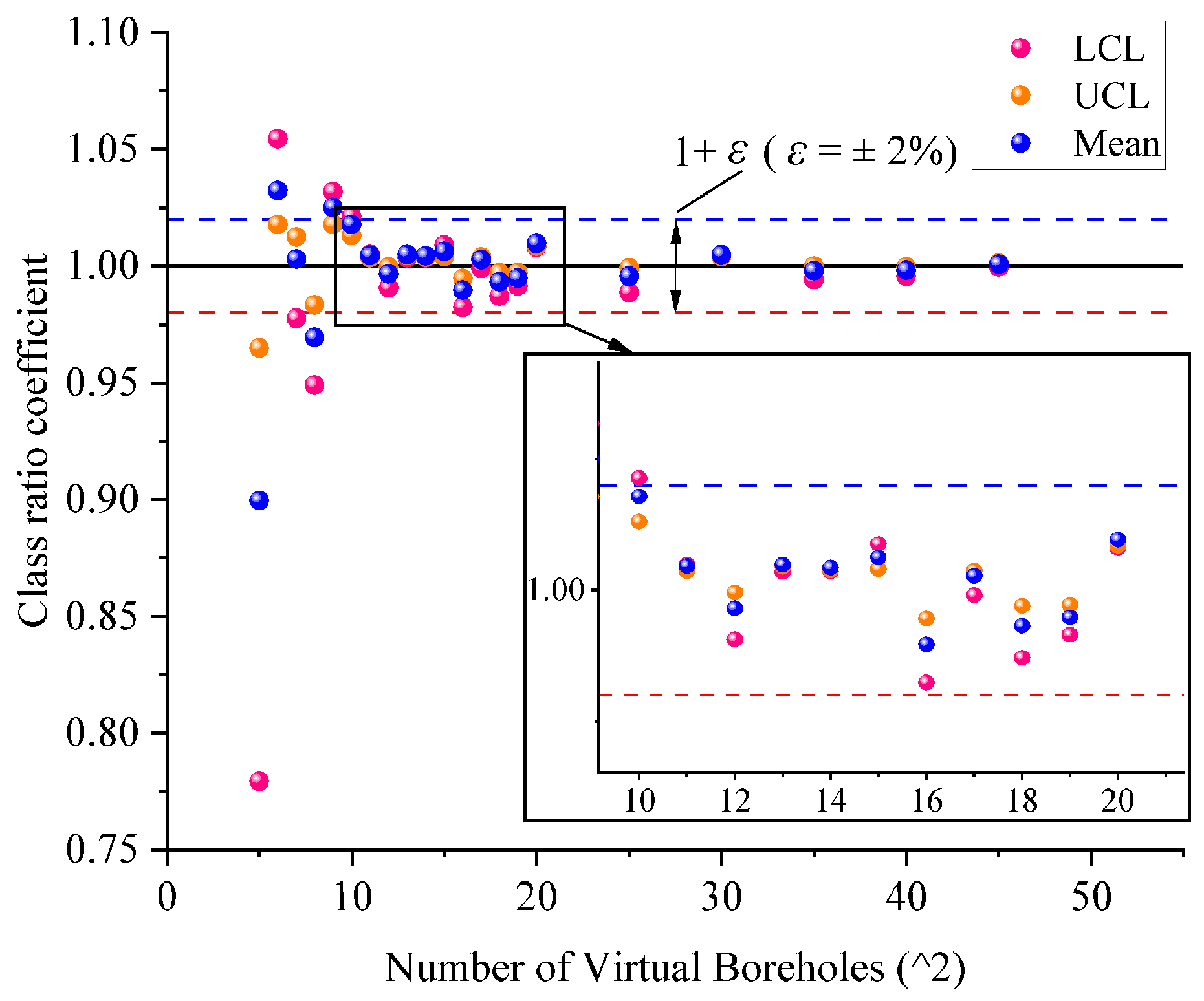
2.2.1. Determining the Thresholds of the Number of Virtual Boreholes
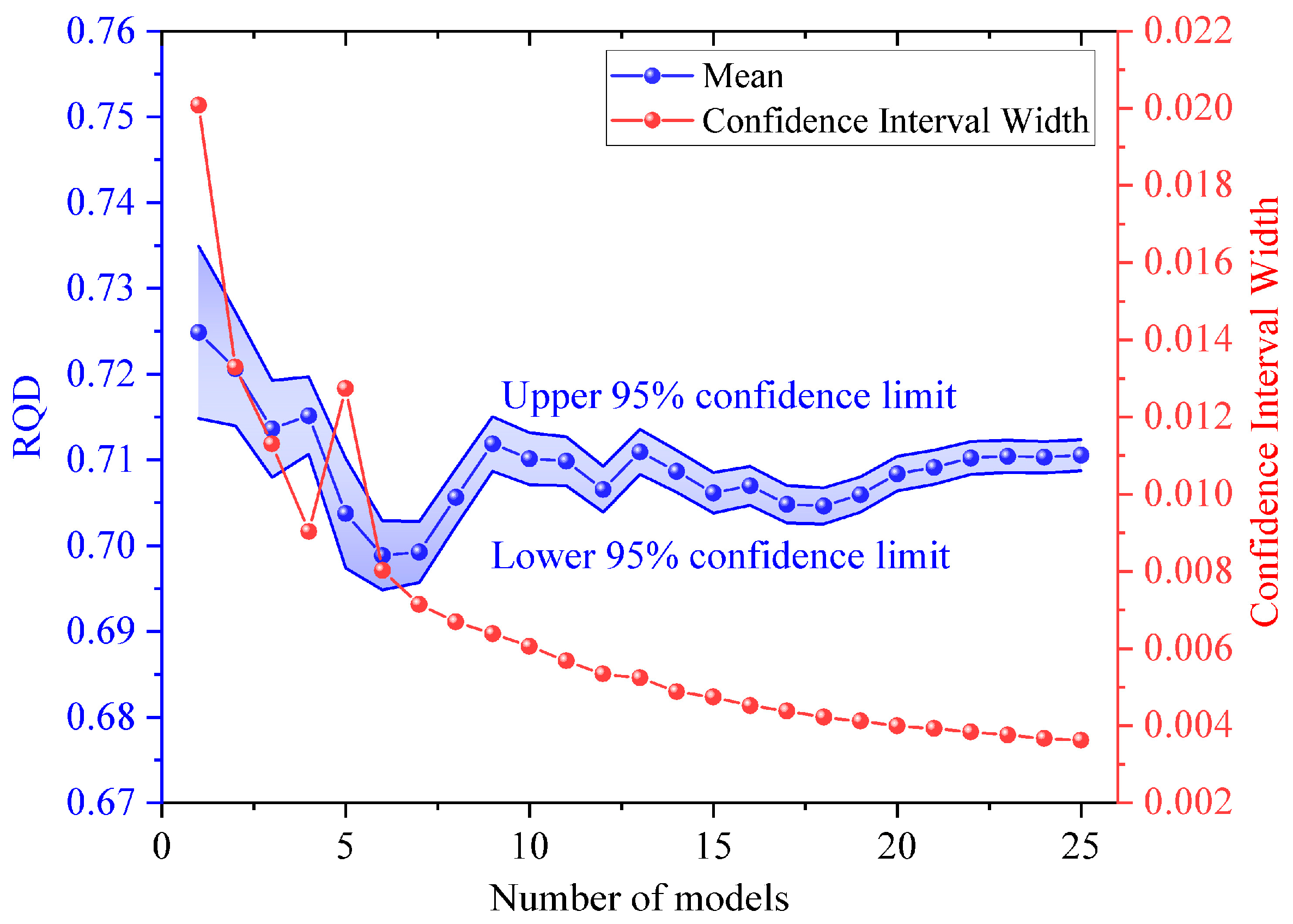
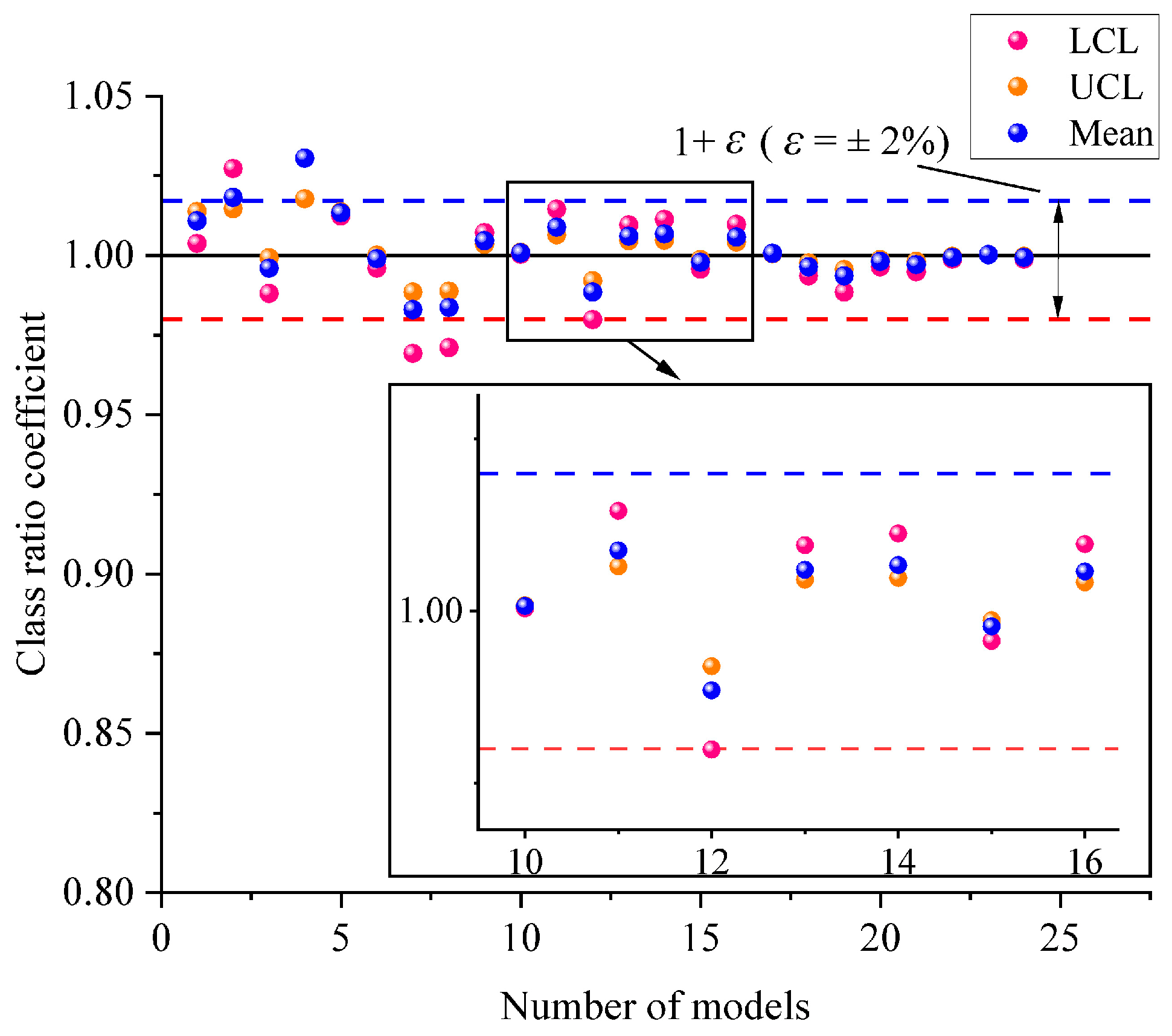
2.2.2. Determining the Thresholds of the Number of Models for a Given Size
2.3. Step 3
2.4. Step 4
3. Case Study
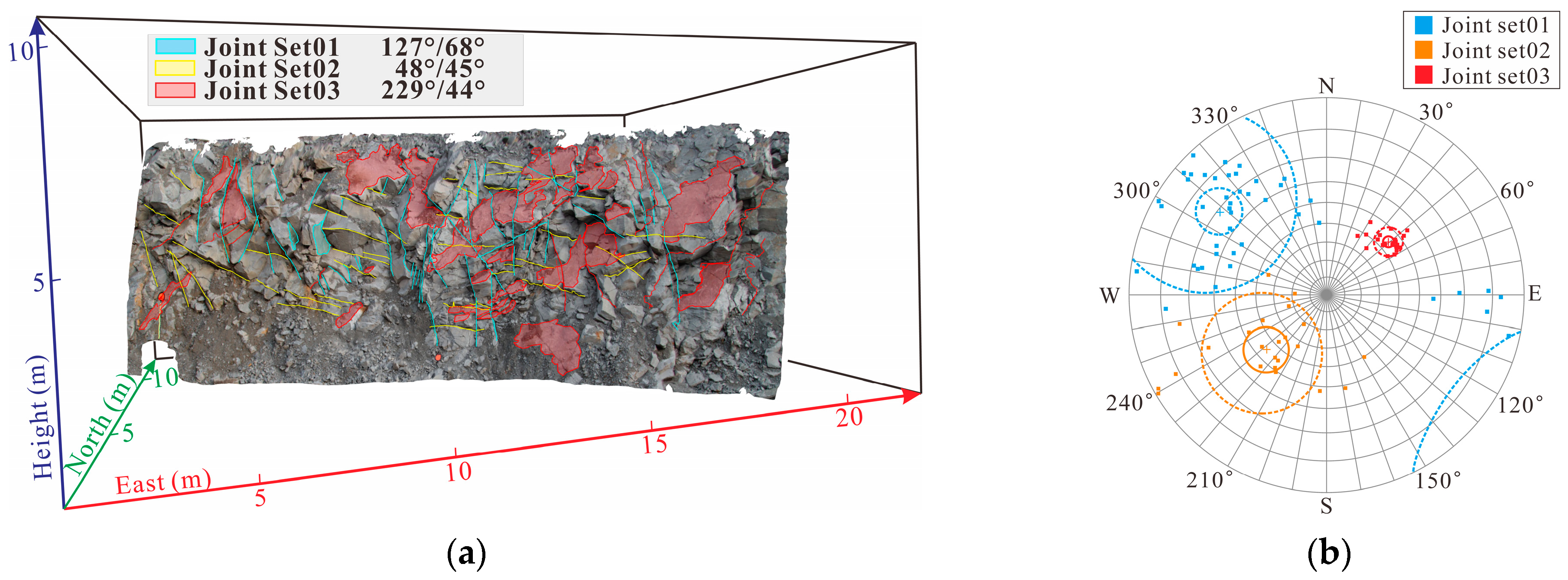
3.1. Study Area
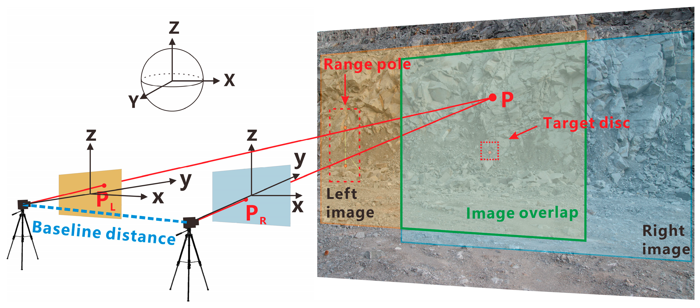
3.2. Geometric Information Acquisition of Rock Mass Discontinuities Based on Photogrammetry
3.3. Selection of Model Size and Number of Virtual Boreholes
4. Results
5. Discussion
6. Conclusions
Author Contributions
Funding
Institutional Review Board Statement
Informed Consent Statement
Data Availability Statement
Acknowledgments
Conflicts of Interest
References
- Brideau, M.-A.; Yan, M.; Stead, D. The role of tectonic damage and brittle rock fracture in the development of large rock slope failures. Geomorphology 2009, 103, 30–49. [Google Scholar] [CrossRef]
- Wu, Q.; Liu, Y.; Tang, H.; Kang, J.; Wang, L.; Li, C.; Wang, D.; Liu, Z. Experimental study of the influence of wetting and drying cycles on the strength of intact rock samples from a red stratum in the Three Gorges Reservoir area. Eng. Geol. 2023, 314, 107013. [Google Scholar] [CrossRef]
- Niu, Q.J.; Jiang, L.S.; Li, C.A.; Zhao, Y.; Wang, Q.B.; Yuan, A.Y. Application and prospects of 3D printing in physical experiments of rock mass mechanics and engineering: Materials, methodologies and models. Int. J. Coal Sci. Technol. 2023, 10, 1–17. [Google Scholar] [CrossRef]
- Feng, F.; Chen, S.; Zhao, X.; Li, D.; Wang, X.; Cui, J. Effects of external dynamic disturbances and structural plane on rock fracturing around deep underground cavern. Int. J. Coal Sci. Technol. 2022, 9, 15. [Google Scholar] [CrossRef]
- Zhang, H.Q.; Zhao, Z.Y.; Tang, C.A.; Song, L. Numerical study of shear behavior of intermittent rock joints with different geometrical parameters. Int. J. Rock Mech. Min. Sci. 2006, 43, 802–816. [Google Scholar] [CrossRef]
- Sun, L.; Grasselli, G.; Liu, Q.; Tang, X.; Abdelaziz, A. The role of discontinuities in rock slope stability: Insights from a combined finite-discrete element simulation. Comput. Geotech. 2022, 147, 104788. [Google Scholar] [CrossRef]
- Zhou, X.; Chen, J.P.; Chen, Y.; Song, S.Y.; Shi, M.Y.; Zhan, J.W. Bayesian-based probabilistic kinematic analysis of discontinuity-controlled rock slope instabilities. Bull. Eng. Geol. Environ. 2016, 76, 1249–1262. [Google Scholar] [CrossRef]
- Wang, X.Q.; Gao, F.Q. Triaxial compression behavior of large-scale jointed coal: A numerical study. Int. J. Coal Sci. Technol. 2022, 9, 76. [Google Scholar] [CrossRef]
- Deere, D.U. Technical description of rock cores for engineering purpose. Rock Mech. Eng. Geol. 1964, 1, 17–22. [Google Scholar]
- Sari, M. The stochastic assessment of strength and deformability characteristics for a pyroclastic rock mass. Int. J. Rock Mech. Min. Sci. 2009, 46, 613–626. [Google Scholar] [CrossRef]
- Zheng, J.; Wang, X.H.; Lü, Q.; Liu, J.F.; Guo, J.C.; Liu, T.X.; Deng, J.H. A Contribution to Relationship Between Volumetric Joint Count (Jv) and Rock Quality Designation (RQD) in Three-Dimensional (3-D) Space. Rock Mech. Rock Eng. 2020, 53, 1485–1494. [Google Scholar] [CrossRef]
- Adarmanabadi, H.R.; Rasti, A.; Mojtabai, N.; Tabaei, M.; Razavi, M. Effects of discontinuities on the rock block geometry of dimension stone quarries: A case study. Geomech. Geoengin. Int. J. 2023. [Google Scholar] [CrossRef]
- Bieniawski, Z. Engineering classification of jointed rock masses. Civ. Eng. Siviele Ingenieurswese 1973, 12, 335–343. [Google Scholar]
- Bieniawski, Z. The rock mass rating (RMR) system (geomechanics classification) in engineering practice. In Rock Classification Systems for Engineering Purposes; Louis, K., Ed.; ASTM: West Conshohocken, PA, USA, 1988. [Google Scholar]
- Barton, N.; Lien, R.; Lunde, J. Engineering classification of rock masses for the design of tunnel support. Rock Mech. 1974, 6, 189–236. [Google Scholar] [CrossRef]
- Takahashi, T.; Takeuchi, T.; Sassa, K. ISRM Suggested Methods for borehole geophysics in rock engineering. Int. J. Rock Mech. Min. Sci. 2006, 43, 337–368. [Google Scholar] [CrossRef]
- Schunnesson, H. RQD predictions based on drill performance parameters. Tunn. Undergr. Space Technol. 1996, 11, 345–351. [Google Scholar] [CrossRef]
- He, M.M.; Li, N.; Yao, X.C.; Chen, Y.S. A New Method for Prediction of Rock Quality Designation in Borehole Using Energy of Rotary Drilling. Rock Mech. Rock Eng. 2020, 53, 3383–3394. [Google Scholar] [CrossRef]
- Zhang, K.; Hou, R.; Zhang, G.; Zhang, G.; Zhang, H. Rock Drillability Assessment and Lithology Classification Based on the Operating Parameters of a Drifter: Case Study in a Coal Mine in China. Rock Mech. Rock Eng. 2016, 49, 329–334. [Google Scholar] [CrossRef]
- Guo, H.-S.; Feng, X.-T.; Li, S.-J.; Yang, C.-X.; Yao, Z.-B. Evaluation of the Integrity of Deep Rock Masses Using Results of Digital Borehole Televiewers. Rock Mech. Rock Eng. 2017, 50, 1371–1382. [Google Scholar] [CrossRef]
- Han, Z.; Wang, C.; Hu, S.; Wang, Y. Application of Borehole Camera Technology in Fractured Rock Mass Investigation of a Submarine Tunnel. J. Coast. Res. 2018, 83, 609–614. [Google Scholar] [CrossRef]
- Falls, S.D.; Young, R.P. Acoustic emission and ultrasonic-velocity methods used to characterise the excavation disturbance associated with deep tunnels in hard rock. Tectonophysics 1998, 289, 1–15. [Google Scholar] [CrossRef]
- Kepic, A.; Kieu, D.T. Relationships between P-Wave Velocity and Rock Quality Designation-A Clustering Perspective. In Proceedings of the 24th European Meeting of Environmental and Engineering Geophysics, Porto, Portugal, 9–12 September 2018. [Google Scholar]
- Priest, S.D.; Hudson, J.A. Estimation of discontinuity spacing and trace length using scanline surveys. Int. J. Rock Mech. Min. Sci. Geomech. Abstr. 1981, 18, 183–197. [Google Scholar] [CrossRef]
- Sen, Z.; Kazi, A. Discontinuity spacing and RQD estimates from finite length scanlines. Int. J. Rock Mech. Min. Sci. Geomech. Abstr. 1984, 21, 203–212. [Google Scholar] [CrossRef]
- Palmstrom, A. Application of the volumetric joint count as a measure of rock mass jointing. In Proceedings of the International Symposium on Fundamentals of Rock Joints, Centek, Luleå, Sweden, 15–20 September 1985. [Google Scholar]
- Boadu, F.K.; Long, L.T. The fractal character of fracture spacing and RQD. Int. J. Rock Mech. Min. Sci. Geomech. Abstr. 1994, 31, 127–134. [Google Scholar] [CrossRef]
- Kayabasi, A.; Yesiloglu-Gultekin, N.; Gokceoglu, C. Use of non-linear prediction tools to assess rock mass permeability using various discontinuity parameters. Eng. Geol. 2015, 185, 1–9. [Google Scholar] [CrossRef]
- Öztürk, C.A.; Nasuf, E. Geostatistical assessment of rock zones for tunneling. Tunn. Undergr. Space Technol. 2002, 17, 275–285. [Google Scholar] [CrossRef]
- Mahmoodzadeh, A.; Mohammadi, M.; Ali, H.F.H.; Abdulhamid, S.N.; Ibrahim, H.H.; Noori, K.M.G. Dynamic prediction models of rock quality designation in tunneling projects. Transp. Geotech. 2021, 27, 100497. [Google Scholar] [CrossRef]
- He, M.M.; Zhao, J.R.; Deng, B.Y.; Zhang, Z.Q. Effect of layered joints on rockburst in deep tunnels. Int. J. Coal Sci. Technol. 2022, 9, 21. [Google Scholar] [CrossRef]
- Li, Y.J.; Song, L.H.; Tang, Y.J.; Zuo, J.P.; Xue, D.J. Evaluating the mechanical properties of anisotropic shale containing bedding and natural fractures with discrete element modeling. Int. J. Coal Sci. Technol. 2022, 9, 18. [Google Scholar] [CrossRef]
- Choi, S.Y.; Park, H.D. Variation of rock quality designation (RQD) with scanline orientation and length: A case study in Korea. Int. J. Rock Mech. Min. Sci. 2004, 41, 207–221. [Google Scholar] [CrossRef]
- Zhang, W.; Wang, Q.; Chen, J.-P.; Tan, C.; Yuan, X.-Q.; Zhou, F.-J. Determination of the optimal threshold and length measurements for RQD calculations. Int. J. Rock Mech. Min. Sci. 2012, 51, 1–12. [Google Scholar] [CrossRef]
- Zhang, W.; Chen, J.; Cao, Z.; Wang, R. Size effect of RQD and generalized representative volume elements: A case study on an underground excavation in Baihetan dam, Southwest China. Tunn. Undergr. Space Technol. 2013, 35, 89–98. [Google Scholar] [CrossRef]
- Ding, Q.; Wang, F.; Chen, J.; Wang, M.; Zhang, X. Research on Generalized RQD of Rock Mass Based on 3D Slope Model Established by Digital Close-Range Photogrammetry. Remote Sens. 2022, 14, 2275. [Google Scholar] [CrossRef]
- Rehman, H.; Kim, J.J.; Yoo, H.K. Stress reduction factor characterization for highly stressed jointed rock based on tunneling data from Pakistan. In Proceedings of the 2017 International Conference on Tunnels and Underground Spaces (ICTUS17), Seoul, Republic of Korea, 28 August–1 September 2017. [Google Scholar]
- Pells, P.J.; Bieniawski, Z.T.; Hencher, S.R.; Pells, S.E. Rock quality designation (RQD): Time to rest in peace. Can. Geotech. J. 2017, 54, 825–834. [Google Scholar] [CrossRef]
- Zhang, Z.; Ye, J. Expression and Analysis of Scale Effect and Anisotropy of Joint Roughness Coefficient Values Using Confidence Neutrosophic Number Cubic Values. Neutrosophic Sets Syst. 2023, 55, 118–131. [Google Scholar] [CrossRef]
- Zhang, S.; Ye, J. Group Decision-Making Model Using the Exponential Similarity Measure of Confidence Neutrosophic Number Cubic Sets in a Fuzzy Multi-Valued Circumstance. Neutrosophic Sets Syst. 2023, 53, 130–138. [Google Scholar] [CrossRef]
- Yong, R.; Huang, L.; Hou, Q.; Du, S. Class Ratio Transform with an Application to Describing the Roughness Anisotropy of Natural Rock Joints. Adv. Civ. Eng. 2020, 2020, 5069627. [Google Scholar] [CrossRef]
- Deng, J. On judging the admissibility of grey modeling via class ratio. J. Grey Syst. 1993, 5, 249–252. [Google Scholar]
- Kun-Li, W.; Jiang-Whai, D.; Ting-Cheng, C.; Chia-Chang, T. The discussions of class ratio for AGO algorithm in grey theory. In Proceedings of the 2001 IEEE International Conference on Systems, Man and Cybernetics. e-Systems and e-Man for Cybernetics in Cyberspace (Cat.No.01CH37236), Tucson, AZ, USA, 7–10 October 2001. [Google Scholar]
- Shen, Y.; Wei, Y. The grey model based on class ratio modeling. In Proceedings of the 2009 Chinese Control and Decision Conference, Guilin, China, 17–19 June 2009. [Google Scholar]
- Yang, B.; Fang, Z.; Zhang, K. Discrete GM (1, 1) model based on sequence of stepwise ratio. Syst. Eng. Electron. 2012, 34, 715–718. [Google Scholar] [CrossRef]
- Sánchez, L.K.; Emery, X.; Séguret, S.A. Geostatistical modeling of Rock Quality Designation (RQD) and geotechnical zoning accounting for directional dependence and scale effect. Eng. Geol. 2021, 293, 106338. [Google Scholar] [CrossRef]
- Lato, M.J.; Vöge, M. Automated mapping of rock discontinuities in 3D lidar and photogrammetry models. Int. J. Rock Mech. Min. Sci. 2012, 54, 150–158. [Google Scholar] [CrossRef]
- Xu, W.; Zhang, Y.; Li, X.; Wang, X.; Ma, F.; Zhao, J.; Zhang, Y. Extraction and statistics of discontinuity orientation and trace length from typical fractured rock mass: A case study of the Xinchang underground research laboratory site, China. Eng. Geol. 2020, 269, 105553. [Google Scholar] [CrossRef]
- Sturzenegger, M.; Stead, D. Close-range terrestrial digital photogrammetry and terrestrial laser scanning for discontinuity characterization on rock cuts. Eng. Geol. 2009, 106, 163–182. [Google Scholar] [CrossRef]
- Gaich, A.; Pötsch, M.; Fasching, A.; Schubert, W. Contact-free measurement of rock mass structures using the jointmetriX3D system. Int. J. Rock Mech. Min. Sci. 2004, 41, 304–309. [Google Scholar] [CrossRef]
- Gaich, A.; Poetsch, M.; Schubert, W. Acquisition and assessment of geometric rock mass features by true 3D images. In Proceedings of the Golden Rocks 2006, the 41st U.S. Symposium on Rock Mechanics (USRMS), Golden, CO, USA, 17–21 June 2006. [Google Scholar]
- Fisher, R.A. Dispersion on a sphere. In Proceedings of the The Royal Society A: Mathematical, Physical and Engineering Sciences (The Royal Society), London, UK, 7 May 1953. [Google Scholar]
- Huang, L.; Tang, H.; Wang, L.; Juang, C.H. Minimum Scanline-to-Fracture Angle and Sample Size Required to Produce a Highly Accurate Estimate of the 3-D Fracture Orientation Distribution. Rock Mech. Rock Eng. 2019, 52, 803–825. [Google Scholar] [CrossRef]
- Warburton, P.M. A stereological interpretation of joint trace data. Int. J. Rock Mech. Min. Sci. Geomech. Abstr. 1980, 17, 181–190. [Google Scholar] [CrossRef]
- Liu, C. Three-Dimensional Fracture Network Modeling of the Rock Mass for Datengxia Water Release Gate Foundation. Master’s Thesis, Jilin University, Jilin, China, 2018. [Google Scholar]
- Lin, J.; Sha, P.; Gao, S.; Ni, J. Characteristics Analysis of Generalized Rock Quality Designation (RQD) Based on Degree of Joint Development. Adv. Civ. Eng. 2021, 2021, 4702348. [Google Scholar] [CrossRef]
- Priest, S.D. Discontinuity Analysis for Rock Engineering, 1st ed.; Chapman & Hall: London, UK, 1993. [Google Scholar]
- Priest, S.D.; Hudson, J.A. Discontinuity spacings in rock. Int. J. Rock Mech. Min. Sci. Geomech. Abstr. 1976, 13, 135–148. [Google Scholar] [CrossRef]
- Bear, J. Dynamics of Fluids in Porous Media, 1st ed.; American Elsevier Publishing Company: New York, NY, USA, 1972. [Google Scholar]
- Wu, Q.; Kulatilake, P.H.S.W. REV and its properties on fracture system and mechanical properties, and an orthotropic constitutive model for a jointed rock mass in a dam site in China. Comput. Geotech. 2012, 43, 124–142. [Google Scholar] [CrossRef]


| Confidence Level (1 − α)% | tα/2 |
|---|---|
| 80% | 1.282 |
| 85% | 1.440 |
| 90% | 1.645 |
| 95% | 1.960 |
| 99% | 2.576 |
| Model Size (m) | n | ξ | β | (1 − α)% | ED(n,α) | ρL(n) | ρU(n) | ρM(n) | WCI |
|---|---|---|---|---|---|---|---|---|---|
| 5 | 25 | 0.771 | 0.067 | 95% | <[0.745, 0.797], 0.771> | 1.091 | 1.108 | 1.100 | 0.052 |
| 49 | 0.701 | 0.065 | 95% | <[0.683, 0.719], 0.701> | 1.000 | 1.008 | 1.004 | 0.036 | |
| 64 | 0.698 | 0.063 | 95% | <[0.683, 0.713], 0.698> | 0.977 | 0.983 | 0.980 | 0.03 | |
| 100 | 0.712 | 0.064 | 95% | <[0.699, 0.725], 0.712> | 1.003 | 1.008 | 1.006 | 0.026 | |
| 144 | 0.708 | 0.065 | 95% | <[0.697, 0.719], 0.708> | 1.003 | 1.008 | 1.006 | 0.022 | |
| 169 | 0.704 | 0.061 | 95% | <[0.695, 0.713], 0.704> | 1.001 | 1.001 | 1.001 | 0.018 | |
| 196 | 0.703 | 0.066 | 95% | <[0.694, 0.712], 0.703> | 0.990 | 0.993 | 0.992 | 0.018 | |
| 225 | 0.709 | 0.065 | 95% | <[0.701, 0.717], 0.709> | - | - | - | 0.016 |
| Group | Average Dip/Dip Angle | Orientation Distribution | Radius Distribution | Linear Density | |||
|---|---|---|---|---|---|---|---|
| Set01 | 127°/68° | Fisher | κ = 17.20 | lognormal | μ | 1.21 | 0.71 |
| σ | 0.36 | ||||||
| Set02 | 48°/45° | Fisher | κ = 22.08 | normal | μ | 2.41 | 0.61 |
| σ | 0.50 | ||||||
| Set03 | 229°/44° | Fisher | κ = 69.20 | lognormal | μ | 1.22 | 1.22 |
| σ | 0.29 | ||||||
| Model Serial Number | Threshold of the Number of Virtual Boreholes | Sample Size for Calculating ED(j,α) | Number of Models | ED(j,α) |
|---|---|---|---|---|
| 1 | 169 | 169 | 1 | <[0.7148, 0.7349], 0.7249> |
| 2 | 169 | 338 | 2 | <[0.7140, 0.7273], 0.7206> |
| 3 | 144 | 482 | 3 | <[0.7080, 0.7193], 0.7136> |
| 4 | 256 | 738 | 4 | <[0.7107, 0.7197], 0.7152> |
| 5 | 196 | 452 | 5 | <[0.6974, 0.7101], 0.7038> |
| 6 | 196 | 1130 | 6 | <[0.6949, 0.7029], 0.6989> |
| 7 | 256 | 1386 | 7 | <[0.6957, 0.7028], 0.6993> |
| 8 | 256 | 1642 | 8 | <[0.7023, 0.7090], 0.7056> |
| 9 | 225 | 1867 | 9 | <[0.7087, 0.7151], 0.7119> |
| 10 | 169 | 2036 | 10 | <[0.7071, 0.7132], 0.7101> |
| 11 | 196 | 2232 | 11 | <[0.7070, 0.7127], 0.7099> |
| 12 | 256 | 2488 | 12 | <[0.7039, 0.7092], 0.7066> |
| 13 | 289 | 2608 | 13 | <[0.7083, 0.7136], 0.7109> |
| 14 | 196 | 2973 | 14 | <[0.7062, 0.7111], 0.7087> |
| 15 | 225 | 3198 | 15 | <[0.7038, 0.7085], 0.7062> |
| 16 | 256 | 3454 | 16 | <[0.7047, 0.7093], 0.7070> |
| 17 | 256 | 3710 | 17 | <[0.7027, 0.7070], 0.7048> |
| 18 | 196 | 3906 | 18 | <[0.7025, 0.7067], 0.7046> |
| 19 | 169 | 4075 | 19 | <[0.7039, 0.7080], 0.7060> |
| 20 | 289 | 4364 | 20 | <[0.7064, 0.7104], 0.7084> |
| 21 | 289 | 4653 | 21 | <[0.7072, 0.7111], 0.7091> |
| 22 | 225 | 4878 | 22 | <[0.7083, 0.7121], 0.7102> |
| 23 | 144 | 5022 | 23 | <[0.7086, 0.7123], 0.7104> |
| 24 | 196 | 5218 | 24 | <[0.7085, 0.7122], 0.7103> |
| 25 | 225 | 5443 | 25 | <[0.7088, 0.7124], 0.7106> |
Disclaimer/Publisher’s Note: The statements, opinions and data contained in all publications are solely those of the individual author(s) and contributor(s) and not of MDPI and/or the editor(s). MDPI and/or the editor(s) disclaim responsibility for any injury to people or property resulting from any ideas, methods, instructions or products referred to in the content. |
© 2023 by the authors. Licensee MDPI, Basel, Switzerland. This article is an open access article distributed under the terms and conditions of the Creative Commons Attribution (CC BY) license (https://creativecommons.org/licenses/by/4.0/).
Share and Cite
Shen, W.; Ni, W.; Yong, R.; Huang, L.; Ye, J.; Luo, Z.; Du, S. Estimating RQD for Rock Masses Based on a Comprehensive Approach. Appl. Sci. 2023, 13, 12855. https://doi.org/10.3390/app132312855
Shen W, Ni W, Yong R, Huang L, Ye J, Luo Z, Du S. Estimating RQD for Rock Masses Based on a Comprehensive Approach. Applied Sciences. 2023; 13(23):12855. https://doi.org/10.3390/app132312855
Chicago/Turabian StyleShen, Wei, Weida Ni, Rui Yong, Lei Huang, Jun Ye, Zhanyou Luo, and Shigui Du. 2023. "Estimating RQD for Rock Masses Based on a Comprehensive Approach" Applied Sciences 13, no. 23: 12855. https://doi.org/10.3390/app132312855
APA StyleShen, W., Ni, W., Yong, R., Huang, L., Ye, J., Luo, Z., & Du, S. (2023). Estimating RQD for Rock Masses Based on a Comprehensive Approach. Applied Sciences, 13(23), 12855. https://doi.org/10.3390/app132312855