Bell-State-Exchange-Parity-Based Protocol for Efficient Autocompensation of Quantum Key Distribution Encoded in Polarization or Spatial Modes

Abstract

We analyze autocompensation possibilities in entanglement-based QKD protocols. In particular, we study the seminal BBM92 protocol and find that an autocompensating technique is possible, although with severe limitations. This prompts the introduction of a different, more practical protocol based on Bell state exchange parity (BSEP), which allows for intrinsic autocompensation of optical fiber perturbations in various two-dimensional fiber-optic encodings while retaining advantageous MDI-QKD characteristics. We present the BSEP protocol in detail, describing both the quantum light propagation and the optical hardware requirements. Finally, we analyze its security, computing its expected performance through the key rate.

1. Introduction

Fast-paced circulation of huge amounts of information across large distances is one of the everyday realities of the Information Age. Importantly, a very significant subset of such information is required, for various motives, to be kept secret.

The bandwidth and distance problem is arguably solved by a crucial piece of optical hardware: optical fibers. As information demands increase, new kinds of fibers, such as multicore fibers (MCFs), have come into play [1], along with few-mode fibers (FMFs) [2,3]. Regarding the secrecy issue, with the advent of quantum computers [4] capable of breaking current public-key cryptosystems, secure methods based on quantum communication have been investigated as a potential solution to such a threat. In particular, quantum key distribution (QKD) is indeed believed to be the ultimate solution to this problem, provided the laws of quantum mechanics are not disputed [5,6]. QKD is one of the most mature fields within the general context of quantum communications, i.e., communications that make use of quantum resources like coherence and entanglement [7] and profit from novel quantum material platforms [8]. However, QKD puts constraints on data bandwidths and achievable distances. This is a consequence of the inherent fragility of the quantum carriers of information: the photons.

In principle, QKD could be implemented in the already available optical fiber infrastructure by using time-bin encoding or polarization, to name perhaps the most famous examples. Moreover, QKD will also benefit from implementations of such new kinds of multicore fibers [9]. Thus, for instance, two- and four-core optical fibers, like the ones recently installed and tested in novel submarine connections [10,11], could be used to perform usual (two-dimensional) QKD. In addition, Hermite–Gauss modes in FMFs could be exploited. QKD would not require a dedicated infrastructure, but some of the fiber systems already deployed could be used.

However, as said, the photon states are fragile. When propagating along a fiber, photons can be lost (scattered, absorbed…) and their quantum states perturbed (modal coupling, phase drifting, dispersion, …). In this paper, apart from losses, we will consider that photonic modes can be coupled between themselves and may pick up a relative phase. The relevant aspect here is that these couplings and/or phases are fundamentally unpredictable. Such fiber perturbations noise-pollute the information encoded in photons, leading to errors in the secret key.

To handle this practically by using already deployed optical fiber technology, and to achieve what has been termed as “plug and play QKD” [12], autocompensation techniques constitute a feasible and simple solution. Different autocompensating systems have been proposed (some of them recently) for polarization perturbations [13], phase perturbations [14], and even general perturbations [15]. This research shows that, via suitable light circulation and application of passive transformations on photonic states, it is possible and practical to cancel optical fiber perturbations of the quantum light states. In this way, QKD protocols can be made robust against both coupling and phase perturbations at a reduced cost. This passive approach towards quantum optical state processing in QKD is not restricted to noise mitigation but also can be applied in other stages of the protocol [16].

A particular challenge is to apply autocompensation to states that are already entangled. As it is well known, there is whole subset of QKD protocols that are entanglement-based, meaning that they employ Bell states from the start and generate keys from the strong quantum correlations captured in such states. Even though production of entangled pairs is not an easy task, entanglement-based QKD has various advantages of its own [17]. Hence, it is desirable to analyze the issue of autocompensation in such protocols, that is, to study the effect of optical fiber perturbations on entangled states and how to remove their undesired effects by autocompensation techniques.

In particular, we will be interested in removing perturbations across various fiber implementations by using polarization modes, for instance, in a single-mode optical fiber (SMF), or two collinear modes in FMFs, or two codirectional modes in MCFs, where Bell states (entangled states) will be excited in two optical fibers. To illustrate the problems associated with entanglement-based QKD, we will focus first on a well-known case: the BBM92 protocol with polarization modes [18]. We will show that only phase drift between optical polarization modes of an SMF can be autocompensated. On the contrary, random simultaneous phases and couplings in the two-dimensional polarization space cannot be autocompensated. A similar situation is found for spatial mode subspaces by using two codirectional or collinear modes of MCFs or FMFs, respectively, and by assuming that there is no cross-polarization. Moreover, we find that such phase drift autocompensation is not simple, and not very favorable in terms of the trade-off between perturbation removal and maximal achievable distance. Therefore, as an alternative, we propose a Bell-state-exchange-parity-based protocol (BSEP, in short), which allows for easy, passive full compensation in both the polarization subspace and spatial subspaces (collinear and codirectional modes), assuming that polarization is maintained under spatial encoding. Moreover, the BSEP protocol has measurement-device-independent (MDI) characteristics [19,20], in line with previous work in the field [21,22,23]. Dealing with the issue of particular attacks in the BSEP protocol, we will show a simple attack that can be launched against the protocol and how to tackle it. Regarding other cases, for instance, a phase-remapping attack [24], which affects bidirectional protocols that encode the information via phase modulation, we shall assume that appropriate ad hoc countermeasures can be applied.

The outline of the paper is as follows: In Section 2, we recall the BBM92 protocol and describe the problems (errors) associated with optical fiber perturbations. We then continue with the phase drift autocompensation technique. In Section 3, we proceed in a similar fashion but with a novel QKD protocol based on Bell state exchange parity. We describe the protocol’s built-in autocompensation technique (general SU(2) perturbations for either polarization or spatial modes), which turns out to be much simpler than for the BBM92 case. In Section 4, we compare both protocols in various scenarios, assessing their performances through a key rate analysis. Finally, the conclusions are presented in Section 5.

2. BBM92 Protocol in 2D Subspace Fiber Encodings

In this section, we briefly address how BBM92 works and show how to generate the required Bell states in spatial-mode encodings (polarization is standard). Next, we present a model of the optical fiber perturbations on the quantum states in the BBM92 protocol. Finally, we describe the autocompensation problems of such protocol.

2.1. Bell States for BBM92 Protocol

Consider the BBM92 protocol [18], where Alice and Bob are separated by some distance and each receive a part of an entangled photonic state. The entangled state comes from a station located in the middle of them. We may call it Charlie, in analogy with MDI-QKD schemes. At Charlie, there is a source emitting singlet states of the form

$$|{\psi }^{-}\rangle =\frac{1}{\sqrt{2}}(|1_{a1}{1}_{b2}\rangle -|1_{a2}{1}_{b1}\rangle ),$$

(1)

This is a maximally entangled Bell state, and moreover, it is a basis-invariant state, as shown below. In principle, we could also use the Bell state $|{\varphi }^{+}\rangle =2^{-1/2}(|1_{a1}{1}_{b1}\rangle +|1_{a2}{1}_{b2}\rangle )$ because $|{\varphi }^{+}\rangle$ is also basis-invariant. Nevertheless, note that the states $|{\psi }^{+}\rangle =2^{-1/2}(|1_{a1}{1}_{b2}\rangle +|1_{a2}{1}_{b1}\rangle )$ and $|{\varphi }^{-}\rangle =(|1_{a1}{1}_{b1}\rangle -|1_{a2}{1}_{b2}\rangle )$ are not basis-invariant, and therefore are less robust than the above states. Nevertheless, $|{\varphi }^{+}\rangle$ and $|{\varphi }^{-}\rangle$ cannot be distinguished by linear optics, which will be important for the protocol we propose later. In short, $|{\psi }^{-}\rangle$ is the optimal choice.

The notation used summarizes any of the encodings under consideration. For instance, $|1_{a1}\rangle$ may be equivalent to $|1_{aH}\rangle$, identifying the state of an H-polarized photon on Alice’s channel, while $|1_{a2}\rangle$ will do so for a V-polarized photon $|1_{aV}\rangle$. Furthermore, the subscripts 1 and 2 identify the cores of a two-core fiber I and $II$, that is, $|1_{aI}\rangle$ and $|1_{aII}\rangle$, as in the usual dual-rail encoding (codirectional modes). Moreover, $|1_{a1}\rangle$ may refer to LP modes in FMFs, which describe a very wide family of modal solutions in optical fibers, that is, $E_{lp}(\rho ,\phi )=F_p\left(\rho \right)e^{il\phi }$, which in turn transport orbital angular momentum l, that is, OAM modes. The radial part determines the type of mode, that is, Hermite–Gaussian modes, Laguerre–Gaussian modes, and so on. For the sake of expositional convenience and without loss of generality, we choose the so-called ${\mathrm{LP}}_{11(\pm )}$ modes. These modes can be expressed as follows: ${\mathrm{LP}}_{11(\pm )}=(1/\sqrt{2})(E_{10}\pm E_{-10})$ which present a zero along the X and Y directions, respectively. Accordingly, we can have single-photon states excited in these modes; that is, $|1_{a1}\rangle$ can refer to $|1_{a+}\rangle \equiv |1_{aX}\rangle$, while $|1_{a2}\rangle$ refers to $|1_{a-}\rangle \equiv |1_{aY}\rangle$. Finally, we could particularize these modes for particular $F\left(\rho \right)$ functions. For example, if the optical fiber admits the radial solution $F\left(\rho \right)=F_o\rho e^{-{\rho }^2/w_o^2}$ (parabolic approximation of a graded index optical fiber), where $w_o$ is a constant and $F_o$ is a normalization constant, the above LP modes become Hermite–Gaussian modes ${\mathrm{H}}_{10}$ and ${\mathrm{H}}_{10}$, where the subindices indicate the number of zeros along the X and Y directions. We will use the notation X and Y for ${\mathrm{LP}}_{11(\pm )}$ modes. Obviously, we could choose other linear combinations, or even the OAM modes $E_{\pm 11}(\rho ,\phi )$, but no new result would be obtained in our study.

We must indicate that we will restrict ourselves to 2D subspaces. For polarization, this is the natural thing to do, but for collinear codirectional modes, we will need to assume that polarization is common to both modes. In terms of actual implementations, the condition of a common polarization is realistic, albeit restrictive, for the case of codirectional modes if we consider, for instance, (multicore) PANDA fibers [25] with reduced polarization mode couplings. For the case of collinear modes, a regular FMF could be used. In this case, it is much more reasonable to assume a common polarization, as the modes travel the same core of the same fiber, although elliptical optical fibers could be used to avoid modal coupling [14].

The reason for treating these different fiber implementations together is that information is actually encoded into isomorphic two-dimensional subspaces. We have two polarization modes, two codirectional modes, and two collinear modes behaving similarly. The general perturbations we consider have formally equivalent expressions, thus allowing us to formally treat the three encodings on the same footing. In other words, the perturbation analysis is the same for all three encodings. It is also desirable to develop a formalism that is as versatile as it is general. The hardware specifics will be different nonetheless.

The BBM92 is a version of the E91 protocol [26], where there is no need to check for a Bell inequality and the usual bases of BB84 [27] are used:

$$\begin{array}{c}\hfill |1_{j1}\rangle =\frac{1}{\sqrt{2}}(|1_{j+}\rangle +|1_{j-}\rangle );|1_{j2}\rangle =\frac{1}{\sqrt{2}}(|1_{j+}\rangle -|1_{j-}\rangle ),j=a,b.\end{array}$$

(2)

Note that the state given by Equation (1) is basis-invariant; that is, it is invariant under the changes given by Equation (2). Moreover, state (1) can be produced by means of a type-I SPDC [28]. For polarization, this is straightforward. For codirectional modes, we need to perform the following: Two biphoton states 1 and 2 are selected. Then, the idler photon of the first biphoton is coupled to the first core of Alice’s fiber and the signal photon is coupled to the second core of Bob’s fiber. At the same time, the idler photon of the second biphoton is coupled to Alice’s fiber’s second core, while the corresponding signal photon is redirected to Bob’s fiber’s first core. In the case of ${\mathrm{LP}}_{11(\pm )}$ modes, we need type II SPDC. In particular, we take the output, separate it with polarizing beam splitters and convert the emerging fundamental Gaussian mode(s) into ${\mathrm{LP}}_{11(\pm )}$ by means of binary phase plates and refractive phase shifters [29]. Then, these are fed into Alice and Bob’s FMFs.

2.2. Perturbations in Quantum Light States

Fibers are imperfect and undergo external perturbations, giving rise to perturbations affecting quantum light states. This means that we will have random relative phases, unpredictable couplings between modes, and even rotations. To model such effects, we assume that we can represent the perturbations as two general SU(2) transformations. These matrices have random parameters, and each one acts locally on Alice’s and Bob’s photonic mode operators. Specifically, we can write the following 4 × 4 matrix, acting on the absorption operator vector ${\{{\widehat{a}}_{a1},{\widehat{a}}_{a2},{\widehat{a}}_{b1},{\widehat{a}}_{b2}\}}^T$

$$P_{ab}=\left(\begin{array}{cccc}{\alpha }_a& -{\overline{\beta }}_a& 0& 0\\ {\beta }_a& \overline{{\alpha }_a}& 0& 0\\ 0& 0& {\alpha }_b& -{\overline{\beta }}_b\\ 0& 0& {\beta }_b& \overline{{\alpha }_b}\end{array}\right).$$

(3)

where the bar stands for conjugation. Therefore, we obtain the following transformation of absorption operators

$${\widehat{a}}_1^{†}\to {\alpha }_j{\widehat{a}}_1^{†}+{\beta }_j{\widehat{a}}_2^{†},{\widehat{a}}_2^{†}\to -{\overline{\beta }}_j{\widehat{a}}_1^{†}+{\overline{\alpha }}_j{\widehat{a}}_2^{†},$$

(4)

where, again, $j=a,b$, as the perturbation coefficients are different for Alice and Bob. Moreover, by recalling the fundamental relationships ${\widehat{a}}_1^{†}|0\rangle =|1_1\rangle$, ${\widehat{a}}_2^{†}|0\rangle =|1_2\rangle$, and by taking into account Equation (4), we see how the singlet state (1) is modified by the action of the perturbations, becoming

$$\begin{array}{c}\hfill |{\psi }^{-}\rangle \to 2^{-1/2}\{({\overline{\beta }}_a{\alpha }_b-{\alpha }_a{\overline{\beta }}_b)|1_{a1}{1}_{b1}\rangle +({\alpha }_a\overline{{\alpha }_b}+{\overline{\beta }}_a{\beta }_b)|1_{a1}{1}_{b2}\rangle \\ \hfill -({\overline{\alpha }}_a{\alpha }_b+{\beta }_a\overline{{\beta }_b})|1_{a2}{1}_{b1}\rangle +({\beta }_a{\overline{\alpha }}_b-{\overline{\alpha }}_a{\beta }_b)|1_{a2}{1}_{b2}\rangle \}.\end{array}$$

(5)

We can already read from here how the perfect (anti-)correlations of the singlet state are disturbed by the perturbations. In fact, whenever Alice and Bob both happen to measure in the Z basis, errors will occur whenever their measurement outcome is $|1_{a1}{1}_{b1}\rangle$ or $|1_{a2}{1}_{b2}\rangle$, which happens with probability

$$p_{err}^Z=1/2({|{\overline{\beta }}_a{\alpha }_b-{\alpha }_a{\overline{\beta }}_b|}^2+{|{\beta }_a{\overline{\alpha }}_b-{\overline{\alpha }}_a{\beta }_b|}^2).$$

(6)

Given that the ideal state is a singlet, either Alice or Bob needs to apply a bit-flip to their measured output. If Alice and Bob’s results are correlated rather than anti-correlated, the bit value will be wrongfully assigned and they will share a string with erroneous bits in such cases. After Alice or Bob broadcasts their choice of basis, each one of them knows that the other one obtained the opposite state. Thus, if everything works fine and Alice measures $|1_{a1}\rangle$, then Bob must have measured $|1_{b2}\rangle$. Alice writes down a 0 as her bit. Bob writes down 1 and bit-flips to 0 (alternatively, it can be Alice who does this). They share the same bit: 0. However, if errors are present, Alice may measure $|1_{a1}\rangle$ and at the same time Bob may measure $|1_{b1}\rangle$. Alice would assign bit 0 and Bob wrotes down 0 and bit-flips to 1, so they no longer share the same string.

Table 1. Expected output measurements for the polarization case in BBM92, for an input state $|{\psi }^{-}\rangle =2^{-1/2}(|1_{aH}{1}_{bV}\rangle -|1_{aV}{1}_{bH}\rangle )$ and in the case of basis agreement (i.e., other events are discarded). Errors correspond to events where the opposite correlation as expected is obtained, which, in the case of perturbations, happens with probabilities given by Equations (6) and (7). Bob is assumed to perform a bit flip.

Basis	Alice’s Outcome	Bob’s Outcome	Bit Agreement
Z	H	V	Correct (bit = 0)
Z	H	H	Error
Z	V	V	Correct (bit = 1)
Z	V	H	Error
X	+	+	Correct (bit = 0)
X	+	−	Error
X	−	−	Correct (bit = 1)
X	−	+	Error

summarizes such situations, also for the X basis, in the polarization encoding for simplicity.

Something similar takes place for measurements in the X basis. First of all, take into account that for this measurement, Alice and Bob need to apply a Hadamard transform first, that is, relationship (2), to their qubits, respectively. Secondly, the state (1) is invariant under a change of basis, so in the X basis, Alice and Bob also expect perfectly anti-correlated results upon measurement. However, the action of the perturbation will prevent this from happening a fraction of the time. Indeed, taking the state (5) and applying the change of basis, we find that errors occur with a probability given by the following expression

$$\begin{array}{c}\hfill p_{err}^X=1/8\left(\right|{\overline{\beta }}_a{\alpha }_b-{\alpha }_a{\overline{\beta }}_b+{\alpha }_a\overline{{\alpha }_b}+{\overline{\beta }}_a{\beta }_b-{\overline{\alpha }}_a{\alpha }_b-{\beta }_a\overline{{\beta }_b}\\ \hfill +{\beta }_a{\overline{\alpha }}_b-{\overline{\alpha }}_a{\beta }_b{|}^2+|{\overline{\beta }}_a{\alpha }_b-{\alpha }_a{\overline{\beta }}_b-{\alpha }_a\overline{{\alpha }_b}-{\overline{\beta }}_a{\beta }_b+{\overline{\alpha }}_a{\alpha }_b\\ \hfill +{\beta }_a\overline{{\beta }_b}+{\beta }_a{\overline{\alpha }}_b-{\overline{\alpha }}_a{\beta }_b{|}^2)\end{array}$$

(7)

These equations will be the basis for our forthcoming error analysis, where we extract error rates from the error probabilities. However, before that, we need to relate the $\alpha$’s and $\beta$’s to more physical parameters [30]. Indeed, writing the perturbation as a matrix, we obtain

$$\begin{array}{c}\hfill P=\left(\begin{array}{cc}\alpha & -\overline{\beta }\\ \beta & \overline{\alpha }\end{array}\right)\\ \hfill \equiv \left(\begin{array}{cc}{e}^{-i(\phi +\omega )/2}cos(\theta /2)& -e^{i(\phi -\omega )/2}sin(\theta /2)\\ e^{-i(\phi -\omega )/2}sin(\theta /2)& e^{i(\phi +\omega )/2}cos(\theta /2)\end{array}\right),\end{array}$$

(8)

We have one such matrix for Alice and another for Bob. This way, we have made it explicit that we have six independent (random) parameters: ${\phi }_a,{\phi }_b,{\omega }_a,{\omega }_b,{\theta }_a,{\theta }_b$. Note that from a more physical point of view, the matrix above can be understood as a general rotation of a quantum state on the Bloch sphere [30].

2.3. The Autocompensation Problem

Let us consider the usual polarization encoding in the BBM92 protocol. By direct inspection, it can be seen that the standard topology, Alice ← Charlie → Bob, of this protocol does not allow the passive autocompensation of cross polarization; not even a simple phase drift can be autocompensated. Indeed, since the quantum source is located at Charlie, the usual round trip technique cannot be used. The only possibility of achieving passive autocompensation would be to change the standard topology. To make this possibility clear, we start by considering the simplified situation where only phase drift exists. This corresponds to the case where the two polarization modes have different propagation constants due to birefringence but without polarization coupling. We will show how to achieve a plug and play topology for autocompensation of phase drifts in Alice’s and Bob’s paths. We insist that polarization modal coupling cannot be autocompensated.

In formal terms, the phase drift can be obtained by setting $\theta =\omega =0$ in Equation (8); therefore, the perturbation becomes simply a phase gate, that is,

$$P_{phase}=\left(\begin{array}{cc}{e}^{-i\phi /2}& 0\\ 0& e^{i\phi /2}\end{array}\right).$$

(9)

Now, if the perturbation takes the form of Equation (9), the error probabilities are much simpler. Indeed, we find that $p_{err}^Z=0$, which makes sense, as phase drift cannot make photons jump between H and V polarizations (and equivalently for the other encodings). The effect of phase drift accumulates relative phases; a bit encoded as $|1_H\rangle$ cannot become $|1_V\rangle$ under the influence of phase drift. This is not the case for a bit encoded as $|1_H\rangle +|1_V\rangle$, which may become the opposite encoded bit if a phase $\pi$ happens to accumulate during propagation, thus producing the state $|1_H\rangle -|1_V\rangle$ (normalization factors aside). Indeed, for the X basis, we obtain

$$p_{err}^X=\frac{1}{2}[1-cos\left(({\phi }_{a2}-{\phi }_{a1})-({\phi }_{b2}-{\phi }_{b1})\right)]=\frac{1}{2}[1-cos({\phi }_a-{\phi }_b)].$$

(10)

that is, states in the X basis are sensible to phase perturbations. Therefore, the entangled state (1) becomes

$$|{\psi }^{-}\rangle =\frac{1}{\sqrt{2}}(e^{i({\phi }_{a1}+{\phi }_{b2})}|1_{a1}{1}_{b2}\rangle +e^{(i({\phi }_{a2}+{\phi }_{b1})}|1_{a2}{1}_{b1}\rangle ),$$

thus accumulating a relative phase $({\phi }_{a2}-{\phi }_{a1})-({\phi }_{b2}-{\phi }_{b1})={\phi }_a-{\phi }_b.$  One can see here that this relative phase does not affect measurements in the Z basis, as the correlations Alice and Bob would measure would remain unchanged.

When postulating probability distributions (PDFs) for these random variables, we shall consider the phase difference ${\phi }_a={\phi }_{a2}-{\phi }_{a1}$ altogether (analogously for ${\phi }_b$). That is, the PDF is a statistical distribution of the phase difference, and not of the individual accumulated phases. This will become clearer in the following sections. We must stress that we maintain the general subscripts $a1,a2,b1,b2$, although for polarization they should be $aH,aV,bH,bV$, whereas the same treatment can be applied to collinear ($X,Y$) codirectional ($I,II$) modes, as mentioned above.

The simplest mechanism in order to passively remove the phase perturbation is to make the modes travel the same path. This way, we obtain a common phase that can be removed. However, in this case, it is not enough to make light travel back and forth, since the state is generated at Charlie but is detected at Alice and Bob. Therefore a plug and play based on a single round trip as used, for instance, in [14,21], is not valid for the BBM92 QKD protocol. It requires as a minimum a triple trip (forth–back–forth). The layout of the fiber-optic circuit implementing autocompensation is shown in Figure 1.

The figure presents two main differences with respect to the single-photon phase autocompensation technique shown in [14]. First, additional circulation/paths are required in BBM92, which greatly increase the propagation distance and thus the attenuation. Secondly, polarization demultiplexing is also required; that is, the H and V modes are separated by a polarizing beam splitter at Charlie and then coupled to polarization-maintaining SMFs. Therefore, the way BBM92 works, it is not possible to devise a phase autocompensation system which, even assuming a maintained polarization, requires less propagation distance than three times the distance between Alice/Bob and Charlie. To briefly see how such a common path can achieve phase autocompensation, take the state (1) but consider the fact that now, due to the common path condition, ${\phi }_{a1}={\phi }_{a2}$ and ${\phi }_{b1}={\phi }_{b2}$. The resulting state is the original state (1), albeit a global phase, and thus the phase perturbation has been autocompensated.

On the other hand, it is clear that general modal-coupling autocompensation is not possible; indeed, if the state starts from the end of Alice and Bob, then, through a round trip, we could formally achieve autocompensation. Still, we need a Bell state shared between Alice an Bob, who are in fact far apart. Consequently, the path between the source and Alice and Bob would be left uncompensated.

In short, polarization perturbations cannot be autocompensated by a single round trip, that is, twice the distance between Alice/Bob and Charlie. However, we achieve phase drift autocompensation via a triple trip, but we must assume that polarization is maintained. This is a strong limitation of the conventional SMFs used in optical fiber networks. Obviously, by using PANDA optical fibers, elliptical optical fibers, and so on, we could notably reduce cross polarization, and thus the triple trip topology could be used.

Finally, we must stress that all the above autocompensation procedures can also be applied to spatial modes, that is, to codirectional modes as long as the cores are so far apart that there is no spatial coupling but they still acquire different phases, or to collinear modes as long as there is no cross talking by using, for instance, elliptical optical fibers. Obviously, polarization must be preserved in all cases. Therefore, it is clear that the BBM92 protocol has very serious intrinsic limitations to be implemented in a plug and play way. Therefore, we will propose a new protocol also based on Bell states but this time with intrinsic advantages that make it applicable to plug and play implementations.

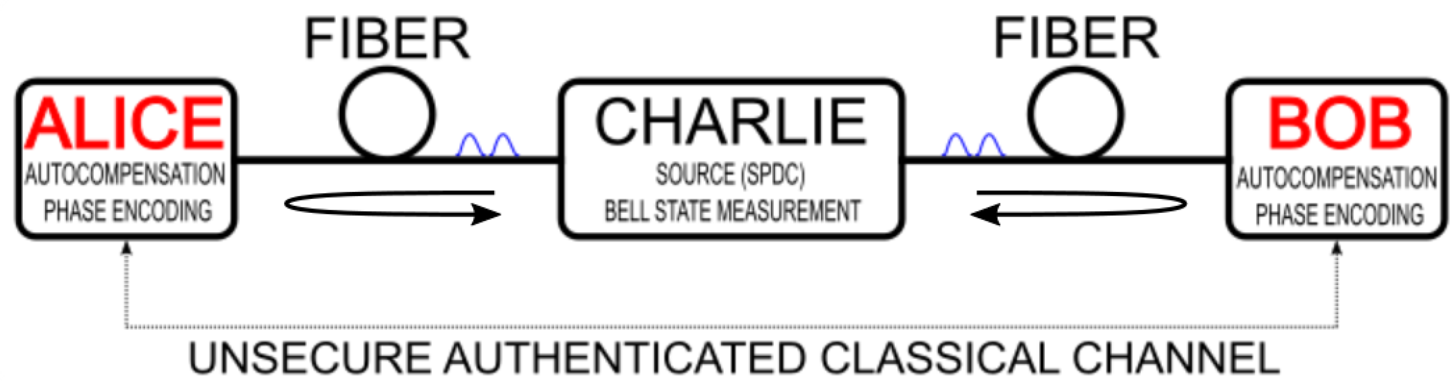
3. Bell State Exchange Parity Protocol and Intrinsic Autocompensation

The analysis performed in the above section shows, through the BBM92 protocol, that QKD based on Bell states, that is, entangled states, presents severe problems when it comes to autocompensation. That is, plug and play based on a single back–forth round trip cannot be used. In order to avoid this drawback, we propose a protocol (see Figure 2) based on Bell state exchange parity (BSEP), conceptually similar to some theoretical QKD idealizations [31]. In our case, we put it in concrete terms, allowing for full intrinsic autocompensation. We must stress that this proposed plug and play protocol with a single round trip is for biphoton entangled states and it also uses three subsystems Charlie–Alice/Bob, which avoids attacks on the photodetection subsystem. In other words, it contains all the advantages of the MDI-QKD protocol. Accordingly, it is fully different from those based on single-photon states [13,14,21] with only two subsystems (Alice/Bob) which are therefore defenseless to attacks on the photodetection subsystem. The physical system implements a protocol with a built-in autocompensation mechanism. In particular, we make use of the states $|{\Psi }^{+}\rangle$ and $|{\Psi }^{-}\rangle$, which can be measured with linear optics. Each encoding requires specific hardware, but they all are conceptually similar. In the case of polarization, we directly use the Innsbruck-type scheme [32], that is, PBSs. Next, we adapt it to the other encodings, as shown in Figure 3. For the case of codirectional modes, Bell state measurements can be performed by means of a small integrated optical circuit, that is, by using two 3dB directional couplers. For collinear modes, the setup is that of polarization, but polarizing beam splitters are substituted with mode-sorting Mach–Zehnder Interferometers (MZIs), which are regular MZIs but with an unrotated Dove prism in one arm (DP${}_0$), that is, with its normal forming an angle equal to 0 with respect to direction Y. Therefore, a phase retarder $\pi$ is produced and consequently, a Z transformation is implemented.

We shall collectively refer to any of these Bell state analyzers as a Bell measurement device (BMD). Photons are bosons, so their overall wavefunction needs to be symmetric. This means that they emerge on different paths at the output of the BMD if they are in any of the (triplet) Bell states or come out in different paths if they are in the singlet state. In practice, this discriminates one Bell state from the others [33]. In other words, Bell state exchange parity produces distinguishable outcomes, and these outcomes can be used to generate a key.

3.1. BSEP Protocol with Polarization Modes

To describe how the BSEP protocol works, without any loss of generality, and to avoid unnecessary repetition, we show the calculations only for polarization encoding. Let us then consider the following input state to the BMD:

$$|L_i\rangle =\begin{array}{c}\hfill \frac{1}{\sqrt{2}}(|1_{aH}{1}_{bV}\rangle +e^{i\theta }|1_{aV}{1}_{bH}\rangle )\end{array},$$

(11)

where the crucial point here is that the phase $\theta ={\theta }_A-{\theta }_B$ can be set by Alice and Bob. Alice chooses randomly the value of ${\theta }_A$ from the set $\{0,\pi \}$ and so does Bob for ${\theta }_B$. In this way, they change the exchange parity of the Bell state.

After going through the device (see Figure 3a), that is, a beam splitter with matrix $H_c=\sqrt{iX}$, with X as the first Pauli matrix, the following state emerges at the output:

$$\begin{array}{c}\hfill \begin{array}{c}\hfill |L_o\rangle =\frac{1}{2\sqrt{2}}[(1-e^{i\theta })|1_{aV}{1}_{bH}\rangle -i(1-e^{i\theta })|1_{aH}{1}_{bV}\rangle +\end{array}\\ \hfill \begin{array}{c}\hfill i(1+e^{i\theta })|1_{aH}{1}_{aV}\rangle +(1+e^{i\theta })|1_{bH}{1}_{bV}\rangle ].\end{array}\end{array}$$

(12)

Now, Alice and Bob have to assign bits to phase choices. A phase choice of 0 is bit 0, and a phase choice of $\pi$ is bit 1. If they choose the same value, then the state (12) becomes

$$\begin{array}{c}\hfill |L_{\theta =0}\rangle =\frac{i}{\sqrt{2}}(|1_{aH}{1}_{aV}\rangle +|1_{bH}{1}_{bV}\rangle ),\end{array}$$

(13)

and thus we have coincidences in either ${\mathrm{D}}_{aH}$ and ${\mathrm{D}}_{bV}$ or ${\mathrm{D}}_{bH}$ and ${\mathrm{D}}_{bV}$ detectors. If they choose a different value,

$$\begin{array}{c}\hfill |L_{\theta =\pm \pi }\rangle =\frac{1}{\sqrt{2}}(|1_{aH}{1}_{bV}\rangle -|1_{aV}{1}_{bH}\rangle ),\end{array}$$

(14)

and thus we have coincidences in either ${\mathrm{D}}_{aH}$ and ${\mathrm{D}}_{bV}$ or ${\mathrm{D}}_{aV}$ and ${\mathrm{D}}_{bH}$ detectors. We call the first case the no-bit-flip case and the second case the bit-flip case.

The measurement is broadcast by Charlie. This endows the protocol with MDI robustness. When they announce a no-bit-flip coincidence, Alice and Bob write down the same bit, which can be 0 or 1. Charlie does not know what case it is, but Alice and Bob do, as they know their own choices. For the bit-flip case, one of them, say Bob, needs to flip their bit. In that case, from the outcome, Charlie cannot guess if the phase choice was ${\theta }_A=0,{\theta }_B=\pi$ (bit 0 on the key) or ${\theta }_A=\pi$ or ${\theta }_B=0$ (bit 1 on the key). With these two pieces of information, the choice of phase and the measurement result, Alice and Bob can write down a shared string of 0 and 1, while Charlie, not privy to the phase choice, would have no information this way. Thus, it is essential that the phase modulators do not leak information outside Alice and Bob’s stations. Note that we assume Alice and Bob to be fully trustworthy; thus, we only have to worry about outside and not inside attacks, as happens in quantum protocols for comparison problems [34,35], where Alice and Bob compete against each other in a sense. Here, in a QKD context, Alice and Bob are assumed to be fully harmless; they are legitimate parties and communicate over a public but authenticated quantum channel (and a companion unjammable classical channel), as is common in a QKD setting. For the case of Charlie, it is untrusted for the measurement; that is, there is no need to make sure that the measurement devices are trusted at all. That is the main contribution of measurement device independence to the QKD field.

Regarding other security aspects, as Charlie is untrusted only for the measurement, there is a possibility of the following individual attack on the input states. In this particular attack, the legitimate input state is supplanted by another of Eve’s desires, a fake state designed to convey information to Eve after Alice and Bob have encoded their information in it, as we will show now. Imagine that Charlie (= Eve) sends, instead of the $|{\psi }^{+}\rangle$ Bell state, a product state of the form

$$\begin{array}{c}\hfill |L_E\rangle =\frac{1}{\sqrt{2}}(|1_{aH}\rangle +|1_{aV}\rangle )\otimes \frac{1}{\sqrt{2}}(|1_{bH}\rangle +|1_{bV}\rangle ).\end{array}$$

(15)

Alice and Bob modulate the relative phase between the polarization components, totally unaware that the state they have received is not what it should be. Thus, what they are actually sending back to Charlie is:

$$\begin{array}{c}\hfill \frac{1}{\sqrt{2}}(|1_{aH}\rangle +e^{i{\theta }_A}|1_{aV}\rangle )\otimes \frac{1}{\sqrt{2}}(|1_{bH}\rangle +e^{i{\theta }_B}|1_{bV}\rangle ).\end{array}$$

(16)

If Eve now directs each qubit to an interferometer, it can retrieve the phases ${\theta }_A$ and ${\theta }_B$ and thus obtain the key bit. For Alice and Bob to notice nothing, Eve has to make a fake announcement at Charlie’s station of the measured output compatible with the relative phase it gleaned.

Fortunately, a simple solution to this attack exists. It requires the sacrifice of some signal pulses. Note that the key rate will be reduced accordingly, but it is far from critical. In order to detect the attack, Alice and Bob have to measure the incoming signal some of the time. If Eve is faking the source signals, they will sometimes obtain results that are incompatible with the state $|{\psi }^{+}\rangle$, for instance, coincidences of the form $|1_{aH}{1}_{bH}\rangle$ and so on. Thus, they will learn, by reporting to each other these measurements via communicating through the classical channel, that Eve has been tampering with the quantum channel.

3.2. Autocompensating BSEP Protocol with Polarization Modes

We must stress that this protocol, due to its two-way architecture, can inherently autocompensate for not only the accumulated propagation phases between $a1$ and $a2$ but also the coupling between them. In a general 2D subspace, perturbations can be removed. The two-way structure means that we now need to consider forward-propagation and back-propagation separately. The reasoning behind autocompensation is that, by means of a simple transformation between round trips, the random coefficients will end up cancelling themselves predictably.

For the case of polarization modes, if the perturbation on the first trip is P (a SU(2) matrix), then when the pulses return, it becomes $P_R=Z{P}^{T}Z$, where T denotes the transpose and Z is the third Pauli matrix. Note that off-diagonal elements change sign, apart from being interchanged [15,21], as the axis of propagation is modified when back-propagating, that is,

$$Z{P}^{T}Z{A}_{p}P=\left(\begin{array}{cc}\alpha & -\beta \\ \overline{\beta }& \overline{\alpha }\end{array}\right)\left(\begin{array}{cc}0& 1\\ 1& 0\end{array}\right)\left(\begin{array}{cc}\alpha & -\overline{\beta }\\ \beta & \overline{\alpha }\end{array}\right)=\left(\begin{array}{cc}0& 1\\ 1& 0\end{array}\right),$$

(17)

where $A_p$ is the polarization autocompensating matrix. This means that while before we had a transformation with unknown, random parameters, we now have a predictable transformation of the quantum state that can easily be reversed. This reversal is deterministic. All the random effects caused by the perturbation are removed automatically by just re-circulating the light back, without the need for active real-time monitoring or calibration. In Figure 4a, we show the device required to implement the above transformation, that is, a half-wave plate (HWP) rotated by $\pi /4$ in a circular circuit. Recall that an $\Omega$-rotated HWP produces the following transformation on polarization modes (albeit containing a global phase which we omit for clarity):

$$HW{P}_{\Omega }=\left(\begin{array}{cc}cos2\Omega & sin2\Omega \\ sin2\Omega & -cos2\Omega \end{array}\right).$$

(18)

The important conclusion is that by a single round trip, any perturbation can be autocompensated, even polarization-dependent absorption can be autocompensated as has been proven [36,37]. The case of a phase drift can be cancelled by a round trip, unlike in the BBM92 protocol, where a triple trip is required and non cross-polarization was assumed.

In order for this autocompensation technique to work, we need to delay pulses in one polarization with respect to the other [13,21] as shown in Figure 2 with two pulses in each path. For instance, the pulse associated with $|1_{jV}\rangle$ is delayed with respect to $|1_{jH}\rangle$ by some fixed quantity $\tau$, that is, $|1_{jV}\rangle$→$|1_{jV\tau }\rangle$. The delay is necessary because we need to separately phase modulate the perturbed $|1_{jH}\rangle$ state with respect to $|1_{jV}\rangle$. If not, the phase $\theta$ we use for information encoding would be mixed in the random state coming out of the fiber. That would be equivalent to introducing a $\theta -$phase gate sandwiched between $A_p$ and P in Equation (20). It is clear that the resulting transformation would not be $A_p$, but another complicated expression involving $\alpha ,\beta$, and $\theta$ altogether; thus, autocompensation would not be achieved. What we actually have, because of the delay, is:

$$\begin{array}{c}\hfill |1_{jH}\rangle \to P_R{A}_{p}P|1_{jH}\rangle =A_p|1_{jH}\rangle ,\\ \hfill |1_{jV}\rangle \to e^{i\theta }{P}_R{A}_{p}P|1_{jV\tau }\rangle =e^{i\theta }{A}_p|1_{jV\tau }\rangle .\end{array}$$

(19)

Thus, correcting for the deterministic transform $A_p$, we restore the original states sent by Charlie. Finally, note that the fact that autocompensation transformation interchanges the pulses; this guarantees that the pulses become synchronous again after traversing the delay when they return to Charlie, that is, $|1_{jH}\rangle \to |1_{jH\tau }\rangle$.

3.3. Autocompensating BSEP Protocol with Spatial Modes

On the other hand, we can use the BSEP protocol with spatial modes (collinear or codirectional) with crosstalk between them in polarization-maintaining fibers (PANDA fibers, elliptical core fibers, and so on). Even the BSEP protocol with spatial modes should be valid in fibers with polarization crosstalk provided the final random polarization is the same in both modes.

If the perturbation for the spatial modes on the first trip is P (a SU(2) matrix), then when the pulses return, it becomes $P_R=P^T$, where T denotes the transpose. Therefore, for spatial modes, we have that [15,21]

$$P^T{A}_{s}P=\left(\begin{array}{cc}\alpha & \beta \\ -\overline{\beta }& \overline{\alpha }\end{array}\right)\left(\begin{array}{cc}0& 1\\ -1& 0\end{array}\right)\left(\begin{array}{cc}\alpha & -\overline{\beta }\\ \beta & \overline{\alpha }\end{array}\right)=\left(\begin{array}{cc}0& 1\\ -1& 0\end{array}\right),$$

(20)

where $A_s$ is the spatial autocompensating matrix. As in the previous polarization-encoding case, the resulting transformation, represented by the matrix above, can easily be accounted for and removed at the end of the process. Thus, again, random perturbations are converted automatically into predictable transformations on the quantum states. On the other hand, note that in the spatial case, the propagation coefficients do not change sign when back-propagating. For autocompensating with spatial modes we must distinguish between collinear and codirectional modes:

• For collinear modes ${\mathrm{LP}}_{11(\pm )}$, for example, HG modes, we use an arrangement of Dove prisms (DPs) rotated suitably, that is, DP${}_{\theta }$, to implement the autocompensating matrix $A_s$. The arrangement of DPs, as shown in Figure 4c, is as follows: First, we have DP${}_0$, that is, a DP with its normal forming an angle equal to 0 with respect to direction Y, producing a phase retarder $\pi$, that is, implementing a Z transformation. Next, we have a DP${}_{-\pi /4}$ implementing a -X transformation; therefore, the total transformation is $-XZ=A_S$ as required. We must stress that cylindrical lens converters (CLCs) can also be used. A CLC is formed by two cylindrical lenses separated by an appropriate distance in such a way that introduces a selective Gouy phase in each spatial direction and therefore a relative phase between ${\mathrm{LP}}_{11(\pm )}$ modes. For HG modes, the design is quite simple [38,39]; however, for other type of modes, the design becomes more complex.
• For the case of codirectional modes, counter-circulation of the modes plus a $\pi$-phase on one of them is enough to produce the desired autocompensating transformation $A_s$, as indicated in Figure 4b; that is, it can be implemented by using two optical circulators and an isotropic $\pi$-phase shifter.

For both spatial mode encodings, we disregard polarization, as commented above, in such a way that we can ignore the contribution of polarization coupling and only worry about spatial coupling. Under these conditions, the state arriving at Charlie will have the following form for codirectional and collinear modes, respectively,

$$|L_{I,II}\rangle =\frac{1}{\sqrt{2}}(|1_{aIp}{1}_{bII{p}^{\prime }}\rangle \pm \left(|1_{aIIp}{1}_{bI{p}^{\prime }}\rangle \right),|L_{X,Y}\rangle =\frac{1}{\sqrt{2}}(|1_{aXp}{1}_{bY{p}^{\prime }}\rangle \pm \left(|1_{aYp}{1}_{bX{p}^{\prime }}\rangle \right)$$

(21)

where p and $p^{\prime }$ denote random polarization states in each path a and b. Note that we assume, in a fair approximation, the same polarization state for each pair of cores: p for Alice and $p^{\prime }$ for Bob.We assume the same for the case of collinear modes, where this assumption is much easily satisfied, as we only have one core. Note that for codirectional modes, when reaching the BMD device, the DCs involved need to be polarization-insensitive; otherwise, coupling phases would be different for modes coming from Alice or from Bob.

As in the case of polarization, a delay must be introduced in one of the pulses before coupling to its core [13,21]. For example, we can delay the pulse associated with $|1_{jII}\rangle$ with respect to $|1_{jI}\rangle$ by some fixed quantity $\tau$. Thus, the equations equivalent to those in Equation (19) are

$$\begin{array}{c}\hfill |1_{jI}\rangle \to P_R{A}_{s}P|1_{jI}\rangle =A_s|1_{jI}\rangle ,\\ \hfill |1_{jII}\rangle \to e^{i\theta }{P}_R{A}_{s}P|1_{jII\tau }\rangle =e^{i\theta }{A}_s|1_{jII\tau }\rangle .\end{array}$$

(22)

Finally, note once again that the autocompensation transformation interchanges the pulses; this guarantees that the pulses become synchronous again after traversing the delay when they return to Charlie, that is, $|1_{jI}\rangle \to |1_{jI\tau }\rangle$.

4. Performance Comparison between Protocols

We now extend the analysis of the errors arising from the perturbations described in the previous sections. The aim is to obtain a final expression of the error rate due to these factors, which can later be introduced into a key rate. With this, we will compare the performance of the BBM92 protocol in various cases: with full perturbations, with only phase perturbations, and with a compensated phase perturbation. In addition, we will see how this relates to the proposed BSEP protocol, which already has a built-in autocompensation mechanism.

To make the expressions of $p_{err}^Z$ and $p_{err}^X$ useful for a key rate analysis, we need to take into consideration that we are considering many rounds of detection. In fact, we will consider the ideal scenario of infinite signals being sent. That is, we need to take the error probabilities $p_{err}^Z$ and $p_{err}^X$ and translate them into actual error rates $e_Z$ and $e_X$. Thus, we need to compute statistical average of the above error probabilities.

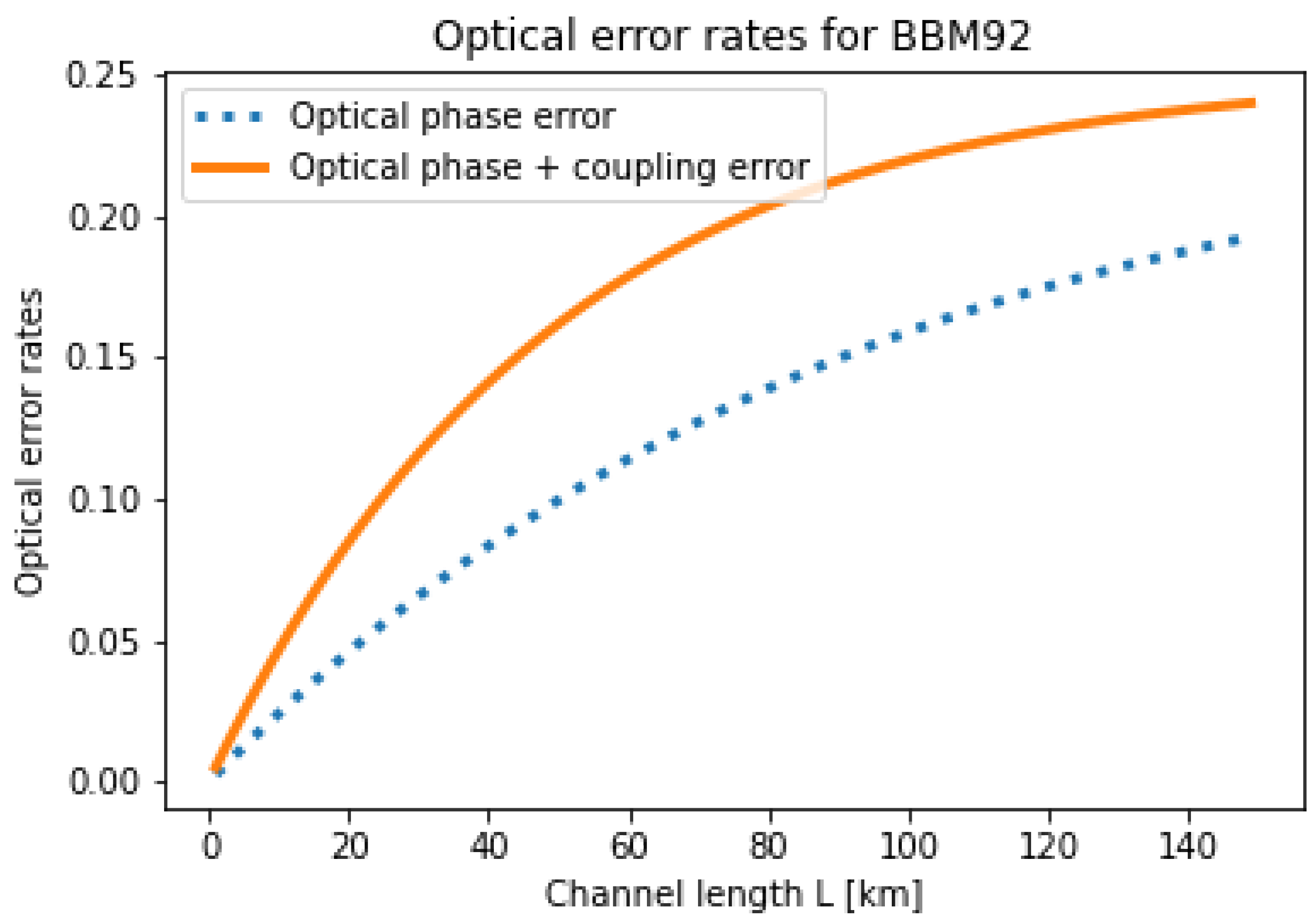
4.1. Optical Perturbation Statistics

As we saw, we have a number of parameters characterizing the perturbation per quantum channel: $\omega$, $\phi$, and $\theta$. As, in general, they are different for Alice and for Bob, we have six different quantities. Now, each of these six parameters is a random variable. We assume that the PDF is separable as a product of probability functions of each of the six variables following Gaussian distributions. Even if it is not always valid, it is very reasonable for the case that we are going to study. Moreover, assuming a Gaussian distribution for the phase is something that has already been considered in the literature [40] in a setting similar to ours. It is also reasonable from the point of view of crosstalk [41]. We assume Gaussians centered at zero for $\delta ={\omega }_a,{\omega }_b,{\phi }_a,{\phi }_b$, taking values between 0 and $2\pi$. We assume that the variance of the distribution is proportional to the propagation length. This way, we can capture the physical fact that the longer the fiber link, the more the perturbation effects accumulate. Furthermore, the specific reason why the proportionality follows $\sigma \propto \sqrt{L}$ assumes that we are dealing with a random walk process [42]. In other words, for the variables above $\delta ={\omega }_a,{\omega }_b,{\phi }_a,{\phi }_b$, we assume the following PDF:

$$p\left(\delta \right)=\frac{1}{\sqrt{N_{\delta }{\gamma }_{\delta }L}}exp[-\frac{1}{2}(\frac{{\delta }^2}{{\gamma }_{\delta }L}\left)\right],$$

(23)

where $N_{\delta }$ is a normalization factor and ${\gamma }_{\delta }$ is the proportionality constant of the variance with L, which measures, in a certain sense, the strength of the perturbation relative to the length scale.

For ${\theta }_a$ and ${\theta }_b$, we need to modify such a distribution and take into account the proper Haar measure [30]. This means that the factor $sin\left(\theta \right)$, with $\theta$ standing for ${\theta }_a$ and ${\theta }_b$, needs to be included in the distribution, with $\theta$ being confined to the range $[0,\pi ]$, that is,

$$p\left(\theta \right)=\frac{sin\theta }{\sqrt{N_{\theta }{\gamma }_{\theta }L}}exp[-\frac{1}{2}(\frac{{\theta }^2}{{\gamma }_{\theta }L}\left)\right],$$

(24)

where $N_{\theta }$ is again another normalization factor. We must stress that the introduction of normalization factors N, beyond the ones that can be computed analytically, allows for computational flexibility, as we can truncate the distribution around values that are found to be highly improbable, i.e., values having negligible contributions to the expected values. This defines a region of interest in which more samples can be allocated, thus optimizing computational resources.

In addition to this, note that, in principle, the $\gamma$s (and the Ns) are different for each variable. To determine a typical value for each of them, we must link the PDF’s variance with experimental data corresponding to codirectional encoding. Note that the off-diagonal terms in Equation (8) are bounded by $sin({\theta }_j/2)$ ($j=a,b$). These terms combine the states $|1_{aI}\rangle$ with $|1_{aII}\rangle$, so ${\gamma }_{\theta a}$ (and similarly ${\gamma }_{\theta b}$) is related with the intercore crosstalk in multicore fibers. This crosstalk decreases with the core pitch, as the overlap between modes of neighbouring cores is reduced. The experimental ratios of power transference range between 10${}^{-4}$ and 10${}^{-6}$ km${}^{-1}$ [43] and are obtained by launching light in a core and measuring the power transferred to the other ones at the fiber exit. These values give us a typical value of ${sin}^2(\theta /2)\simeq {\theta }^2/4$. Thus, we consider ${\gamma }_{\theta a}={\gamma }_{\theta b}\simeq 5\times {10}^{-5}$ km${}^{-1}$. Since $\theta$ is small in Equation (8), $\phi$ and $\omega$ are directly related to the relative phase between the modes of both cores. The propagation time difference (skew) in the two cores of a 53 km-long multicore fiber was found to fluctuate in the order of picoseconds in a laboratory experiment at a stabilized temperature [44]. In terms of phase, this corresponds to huge phase excursions of around 400$\pi$ and therefore to a value of ${\gamma }_{\omega }={\gamma }_{\phi }\sim 3\times {10}^4$ km${}^{-1}$. Consequently, $\omega$ and $\phi$ are fully random in the wrapped range [0, 2$\pi$) for typical propagation distances in QKD. Since this effect is dominant, we even could neglect the dispersion of $\theta$ in Equation (8), which reduces to (9) with a completely random phase; consequently, Equation (10) predicts that X-base measurements provide no information at all: $〈p_{err}^X〉=1/2$. The original BBM92 protocol does not work in this passive encoding due to the phase noise introduced by the fiber. In polarization encoding, the evolution of the perturbations is different. The fiber can be modeled as a succession of sections with randomly oriented residual anisotropies [43]. The amount of random anisotropy can be estimated from the polarization mode dispersion of the optical fiber as 0.04 ps/$\sqrt{\mathrm{km}}$ in a good modern fiber. This leads to a somewhat better dispersion of $\omega$ (${\gamma }_{\omega }\sim 2.5\times {10}^3$ rad${}^2$/km); however, it is still too high to be useful. Moreover, unlike the previous case, the final transformation is now completely arbitrary for typical propagation distances. Finally, a similar situation is to be expected with respect to collinear encoding, since crosstalk between degenerate spatial modes is important in modern few-mode fibers.

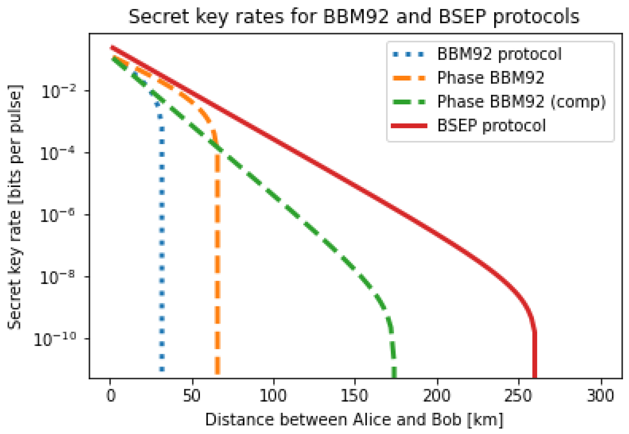
4.2. Simplified Security Analysis

We now analyze the impact of the perturbation-motivated errors on the key rate. As this paper is focused on optical hardware for QKDs, it will be enough to present an elemental security analysis. Recall that in the first place, we assumed Alice and Bob exchange an infinite number of single-photon signals. We shall follow [17] and, more specifically, the simple case contained in it. We also assume a symmetric channel, where detector efficiencies, attenuation, and dark counts are the same for Alice and Bob. We use a basic version of the key rate, emphasizing the errors due to perturbations and assuming that Eve does not have any information about the basis used for measurement, so the bit error rate and the phase error rates are equal [17,45]. With these conditions, the secret key rate is given by [45]

$$R\ge q{Y}_{11}[1-fH\left(e_{11}\right)-H\left(e_{11}\right)].$$

(25)

where the meanings of the parameters contained in the equation above are the following: q is the base-sift factor ($q=1/2$ for BBM92, $q=1$ for BSEP); $Y_1$ is the single-photon yield, given by

$$Y_{11}=[1-(1-Y_0)(1-\eta )]{,}^2$$

(26)

where $Y_0$ is the dark-count-associated yield and $\eta$ is the product of the channel transmissivity, depending on channel length L, attenuation ${\alpha }_{att}$ (given by ${10}^{-{\alpha }_{att}L/10}$), and the detector efficiency ${\eta }_d$. Therefore, $\eta ={\eta }_d{10}^{-{\alpha }_{att}L/10}$. Moreover, we consider that the attenuation along the Alice–Charlie and Bob–Charlie paths (each of length L) is the same. The value of $\eta$ roughly represents the probability of detecting a photon at the end of a lossy fiber at a detector of efficiency ${\eta }_d$. Furthermore, we assume that every detector has the same dark count probability.

$e_{11}$ is the single-photon error, which can be estimated from the measured error rates on the Z and X basis [45] as $e_{11}=(e_x+e_z)/2$. This error has three contributions: one due to the perturbations, which we indicate as $E_{opt}$ (optical error); another due to the dark counts; and a third one, a residual error term $e_{res}$, that accounts for additional sources of errors not included in the perturbations. When we compensate for the perturbations, then $E_{opt}=0$. Regarding the physical causes of the residual error, they may be due to misalignments in the measuring apparatus. This particular error we cannot eliminate even when we autocompensate the protocol, but we expect it not to be too big if the optical hardware is reliable enough. We use a typical value of $e_{res}=1.5\%$ [46]. We emphasize that the addition of such a residual term, if small, does not affect our conclusions regarding the benefits of autocompensation, as it is common in every protocol. With all of this in place, the single-photon error becomes

$$e_{11}=e_0(1-\frac{{\eta }^2}{Y_{11}})+\frac{(E_{opt}+e_{res}){\eta }^2}{Y_{11}}.$$

(27)

Finally, H is the well-known binary Shannon entropy, given by the following formal expression

$$H\left(x\right)=-x{log}_{2}x-(1-x){log}_2(1-x).$$

(28)

We must recall that the error rate is the fraction of erroneous events (detector misfires) in the total events; therefore, the interpretation of Equation (27) is as follows. We have two separate contributions: On the one hand, the optical error contribution (plus the residual term) occurs with fraction ${\eta }^2/Y_{11}$, that is, the probability ${\eta }^2$ of coincidences of two photons over the probability that two photons arrive at the detectors, given that Charlie produces a two-photon entangled state. On the other hand, dark counts contribute when no photon arrives at the detectors but clicks happen nonetheless; this rate is reduced whenever dark counts and true coincidences happen at the same time (this being a case that happens with so negligible a probability that it is usually disregarded [17]).

The use of this key rate amounts to the assumption that the sources are perfect and single-photon, while the other components (fibers and detectors) are imperfect. This is not entirely true, but we want to focus on the imperfections of the fiber link. Moreover, to compute (26), we assume that we can model the optical signal loss as a beam splitter (BS) on the channel [20], followed by perfect detectors (detector efficiency is included in the losses). One of the ports of the BS has a vacuum input; the input of the other port is the optical signal. One of the exit ports leaks photons to the environment, while the other is the channel ‘mode’. If we compute the density operator of this mode and trace out the environment, we can find the yield $Y_{11}$ (which, in this case, is equal to the gain as the source is perfect, that is, $p\left(\mathrm{single}\mathrm{photon}\mathrm{emission}\right)=1$) as the quantity $1-p\left(\mathrm{no}\mathrm{click}\right)$, with p meaning the probability. If we include dark counts and take into account that we are computing coincidences, we have $Y_{11}={[1-(1-Y_0)(1-\eta )]}^2.$

As said, we considered different scenarios. The first one is the BBM92 protocol with full perturbations. In this case, we need to compute the expected values of Equations (6) and (7) with the PDFs above. We have that

$$E_{opt}=\frac{\langle p_{err}^Z\rangle +\langle p_{err}^X\rangle }{2}.$$

(29)

Note that for each value of the channel length L (with total achievable distance equal to $2L$), the variance of the PDFs is different. The results are plotted in Figure 5. Along this error rate, we plot the error rate due only to phase perturbations, that is, the quantity

$$E_{opt}^{phase}=\frac{1}{2}\langle p_{err}^X\rangle ,$$

(30)

where, in this case, $p_{err}^X$ is given by Equation (10).

Next, we evaluate the secret key rate as a function of distance using Equation (25). For the autocompensating case, we formally have ${\gamma }_{\delta }={\gamma }_{\theta }=0$. For the non autocompensating case, we have already made estimations in the previous section, that is, ${\gamma }_{\theta }\approx 5\times {10}^{-5}$ km${}^{-1}$, but ${\gamma }_{\delta }$ has huge values experimentally. Nevertheless, in order to make the critical effect of optical fiber perturbations clear, although they will become quite small, we will assume the following hypothetical value: ${\gamma }_{\delta }\approx 3\times {10}^{-2}$ km${}^{-1}$, that is, six orders of magnitude smaller than the real perturbation. Finally, for attenuation, we assume a value of 0.15 dB/km. For the detector efficiency, we assume ${\eta }_d=60\%$. The dark count yield is $Y_0=6.02\times {10}^{-6}$. Finally, for the error inefficiency, given the values of our errors, we take a pessimistic [47] $f=1.35$ value.

In Figure 5, the variation in the optical error with the distance is shown, which is in turn used to obtain the results shown in Figure 6. We must emphasize that the curves of the secret key rate are critically influenced by the value of fiber attenuation. In fact, if this parameter becomes large enough, then protocols where the light needs to travel longer distances, for example, in BBM92, in order to achieve phase autocompensation exhibit a significant reduction in the secret key rate. On the other hand, without autocompensation, the maximum transmission distances to achieve a secure secret key are relatively short (a few tens of kilometers, as shown by the blue and orange curves in Figure 6), despite having used hypothetical, small values for the phase drift. Therefore, for real optical fibers, such distances would be reduced by up to a few meters. If we use an autocompensated BBM92 protocol, longer distances are achieved (green curve); however, with the plug and play BSEP protocol, much longer transmission distances are obtained, which is the central result of this work.

5. Conclusions

We have examined the BBM92 protocol and shown that, in this case (and quite possibly others like it), autocompensation is either not possible (full perturbation) or not a very good solution even for simpler cases (phase). As an alternative, we have proposed another entanglement-based QKD protocol making use of the exchange parity of Bell states. Such a protocol has a simple, built-in autocompensation mechanism that allows transmission of the secure key over longer distances at a larger rate. Moreover, by construction, the BSEP protocol has MDI characteristics. This extends previous work [21] addressing purely MDI protocols, where entanglement occurred only at the final time upon measurement by postselection, or more conventional plug and play versions of the BB84 protocol [12], which are not robust in general against detection side-channel attacks. We believe that the BSEP protocol does not introduce new backdoors for an eavesdropper to take advantage of, apart from the proposed attack, for which we present a simple way to tackle. That said, the protocol we propose is not free from other attacks common to such classes of MDI-QKD protocols. In particular, the MDI protocol is still vulnerable to other attacks, except those on the measurement system, for example, the source [48], as the MDI protocol does not provide full device independence as DI-QKD does [49], which nonetheless remains experimentally challenging. At the present time, MDI protocols remain the most feasible QKD protocols that are able to avoid a general class of attacks; thus, the interest in working on such a direction, as we did, is high. To compare BBM92 with the new BSEP protocol, we have analyzed the relevant perturbation errors. We have conducted a simplified but clarifying security analysis by introducing these errors into a simple version of the key rate, taking into account real-life optical hardware imperfections such as fiber attenuation, detector inefficiency, and detector dark counts. In short, the proposed QKD protocol inherently removes coupling and phase perturbations in two-mode fiber-optic systems, overcoming prior problems associated with the direct use of entangled states for information encoding, such as in the BBM92 protocol.

References

1. Saitoh, K.; Matsuo, S. Multicore Fiber Technology. J. Light. Technol. 2016, 34, 55–66. [Google Scholar] [CrossRef]
2. Berdagué, S.; Facq, P. Mode division multiplexing in optical fibers. Appl. Opt. 1982, 21, 1950–1955. [Google Scholar] [CrossRef] [PubMed]
3. Sillard, P.; Bigot-Astruc, M.; Molin, D. Few-Mode Fibers for Mode-Division-Multiplexed Systems. J. Light. Technol. 2014, 32, 2824–2829. [Google Scholar] [CrossRef]
4. Shor, P. Algorithms for quantum computation: Discrete logarithms and factoring. In Proceedings of the 35th Annual Symposium on Foundations of Computer Science, Santa Fe, NM, USA, 20–22 November 1994; pp. 124–134. [Google Scholar] [CrossRef]
5. Gisin, N.; Ribordy, G.; Tittel, W.; Zbinden, H. Quantum cryptography. Rev. Mod. Phys. 2002, 74, 145–195. [Google Scholar] [CrossRef]
6. Pirandola, S.; Andersen, U.L.; Banchi, L.; Berta, M.; Bunandar, D.; Colbeck, R.; Englund, D.; Gehring, T.; Lupo, C.; Ottaviani, C.; et al. Advances in quantum cryptography. Adv. Opt. Photon. 2020, 12, 1012–1236. [Google Scholar] [CrossRef]
7. Kelly, S.P.; Poschinger, U.; Schmidt-Kaler, F.; Fisher, M.P.A.; Marino, J. Coherence requirements for quantum communication from hybrid circuit dynamics. arXiv 2023, arXiv:2210.11547. [Google Scholar]
8. Bashir, A.I. Quantum coherence-assisted secure communication of internet of things information via Landau-quantized graphene. Opt. Quantum Electron. 2023, 55, 983. [Google Scholar] [CrossRef]
9. Xavier, G.B.; Lima, G. Quantum information processing with space-division multiplexing optical fibres. Commun. Phys. 2020, 3, 9. [Google Scholar] [CrossRef]
10. Boosting Subsea Cables with Multi-Core Fiber Technology. Available online: https://cloud.google.com/blog/products/infrastructure/delivering-multi-core-fiber-technology-in-subsea-cables (accessed on 13 September 2023).
11. Takeshita, H.; Nakamura, K.; Matsuo, Y.; Inoue, T.; Masuda, D.; Hiwatashi, T.; Hosokawa, K.; Inada, Y.; de Gabory, E.L.T. First Demonstration of Uncoupled 4-Core Multicore Fiber in a Submarine Cable Prototype with Integrated Multicore EDFA. In Proceedings of the Optical Fiber Communication Conference (OFC) 2022, San Diego, CA, USA, 6–10 March 2022; p. M4B.1. [Google Scholar] [CrossRef]
12. Muller, A.; Herzog, T.; Huttner, B.; Tittel, W.; Zbinden, H.; Gisin, N. “Plug and play” systems for quantum cryptography. Appl. Phys. Lett. 1997, 70, 793–795. [Google Scholar] [CrossRef]
13. Bethune, D.S.; Risk, W.P. Autocompensating quantum cryptography. New J. Phys. 2002, 4, 42. [Google Scholar] [CrossRef]
14. Balado, D.; Liñares, J.; Prieto-Blanco, X.; Barral, D. Phase and polarization autocompensating N-dimensional quantum cryptography in multicore optical fibers. J. Opt. Soc. Am. B 2019, 36, 2793–2803. [Google Scholar] [CrossRef]
15. Liñares, J.; Prieto-Blanco, X.; Balado, D.; Carral, G.M. Fully autocompensating high-dimensional quantum cryptography by quantum degenerate four-wave mixing. Phys. Rev. A 2021, 103, 043710. [Google Scholar] [CrossRef]
16. Zapatero, V.; Wang, W.; Curty, M. A fully passive transmitter for decoy-state quantum key distribution. Quantum Sci. Technol. 2023, 8, 025014. [Google Scholar] [CrossRef]
17. Ma, X.; Fung, C.H.F.; Lo, H.K. Quantum key distribution with entangled photon sources. Phys. Rev. A 2007, 76, 012307. [Google Scholar] [CrossRef]
18. Bennett, C.H.; Brassard, G.; Mermin, N.D. Quantum cryptography without Bell’s theorem. Phys. Rev. Lett. 1992, 68, 557–559. [Google Scholar] [CrossRef] [PubMed]
19. Lo, H.K.; Curty, M.; Qi, B. Measurement-Device-Independent Quantum Key Distribution. Phys. Rev. Lett. 2012, 108, 130503. [Google Scholar] [CrossRef] [PubMed]
20. Ma, X.; Razavi, M. Alternative schemes for measurement-device-independent quantum key distribution. Phys. Rev. A 2012, 86, 062319. [Google Scholar] [CrossRef]
21. Liñares, J.; Carral, G.M.; Prieto-Blanco, X.; Balado, D. Autocompensating measurement-device-independent quantum cryptography in space division multiplexing optical fibers. J. Eur. Opt. Soc. Rapid Publ. 2021, 17, 19. [Google Scholar] [CrossRef]
22. Park, C.H.; Woo, M.K.; Park, B.K.; Lee, M.S.; Kim, Y.S.; Cho, Y.W.; Kim, S.; Han, S.W.; Moon, S. Practical Plug-and-Play Measurement-Device-Independent Quantum Key Distribution With Polarization Division Multiplexing. IEEE Access 2018, 6, 58587–58593. [Google Scholar] [CrossRef]
23. Hu, M.; Zhang, L.; Guo, B.; Li, J. Polarization-based plug-and-play measurement-device-independent quantum key distribution. Opt. Quantum Electron. 2019, 51, 22. [Google Scholar] [CrossRef]
24. Fung, C.H.F.; Qi, B.; Tamaki, K.; Lo, H.K. Phase-remapping attack in practical quantum-key-distribution systems. Phys. Rev. A 2007, 75, 032314. [Google Scholar] [CrossRef]
25. Yang, Y.; Gao, J.; Fu, S.; Zhang, X.; Tang, M.; Tong, W.; Liu, D. PANDA Type Four-Core Fiber With the Efficient Use of Stress Rods. IEEE Photonics J. 2019, 11, 1–9. [Google Scholar] [CrossRef]
26. Ekert, A.K. Quantum cryptography based on Bell’s theorem. Phys. Rev. Lett. 1991, 67, 661–663. [Google Scholar] [CrossRef] [PubMed]
27. Bennet, C.H.; Brassard, G. Quantum Cryptography: Public key distribution and coin tossing. In Proceedings of the IEEE International Conference on Computers, Systems and Signal Processing, Bangalore, India, 9–12 December 1984; pp. 175–179. [Google Scholar]
28. Kwiat, P.G.; Waks, E.; White, A.G.; Appelbaum, I.; Eberhard, P.H. Ultrabright source of polarization-entangled photons. Phys. Rev. A 1999, 60, R773–R776. [Google Scholar] [CrossRef]
29. Liñares, J.; Prieto-Blanco, X.; Moreno, V.; Montero-Orille, C.; Mouriz, D.; Nistal, M.C.; Barral, D. Interferometric space-mode multiplexing based on binary phase plates and refractive phase shifters. Opt. Express 2017, 25, 10925–10938. [Google Scholar] [CrossRef] [PubMed]
30. Understanding the Haar Measure. Available online: https://pennylane.ai/qml/demos/tutorial_haar_measure.html#understanding-the-haar-measure (accessed on 19 April 2023).
31. Wang, X.B.; Yu, Z.W.; Hu, X.L. Twin-field quantum key distribution with large misalignment error. Phys. Rev. A 2018, 98, 062323. [Google Scholar] [CrossRef]
32. Mattle, K.; Weinfurter, H.; Kwiat, P.G.; Zeilinger, A. Dense Coding in Experimental Quantum Communication. Phys. Rev. Lett. 1996, 76, 4656–4659. [Google Scholar] [CrossRef]
33. Weihs, G.; Zeilinger, A. Photon Statistics at Beam Splitters: An Essential Tool in Quantum Information and Teleportation; 2001. Available online: https://api.semanticscholar.org/CorpusID:174794052 (accessed on 9 October 2023).
34. Wu, W.; Zhou, G.; Zhao, Y.; Zhang, H. New Quantum Private Comparison Protocol Without a Third Party. Int. J. Theor. Phys. 2020, 59, 1866–1875. [Google Scholar] [CrossRef]
35. Huang, X.; Zhang, S.B.; Chang, Y.; Hou, M.; Cheng, W. Efficient Quantum Private Comparison Based on Entanglement Swapping of Bell States. Int. J. Theor. Phys. 2021, 60, 3783–3796. [Google Scholar] [CrossRef]
36. Martinelli, M. A universal compensator for polarization changes induced by birefringence on a retracing beam. Opt. Commun. 1989, 72, 341–344. [Google Scholar] [CrossRef]
37. Bhandari, R. A useful generalization of the Martinelli effect. Opt. Commun. 1992, 88, 1–5. [Google Scholar] [CrossRef]
38. Beijersbergen, M.; Allen, L.; van der Veen, H.; Woerdman, J. Astigmatic laser mode converters and transfer of orbital angular momentum. Opt. Commun. 1993, 96, 123–132. [Google Scholar] [CrossRef]
39. Liñares, J.; Prieto-Blanco, X.; Montero-Orille, C.; Moreno, V. Spatial mode multiplexing/demultiplexing by Gouy phase interferometry. Opt. Lett. 2017, 42, 93–96. [Google Scholar] [CrossRef] [PubMed]
40. Dellantonio, L.; Sorensen, A.S.; Bacco, D. High-dimensional measurement-device-independent quantum key distribution on two-dimensional subspaces. Phys. Rev. A 2018, 98, 062301. [Google Scholar] [CrossRef]
41. Ng, K.; Nazarov, V.; Kuchinsky, S.; Zakharian, A.; Li, M.J. Analysis of Crosstalk in Multicore Fibers: Statistical Distributions and Analytical Expressions. Photonics 2023, 10, 174. [Google Scholar] [CrossRef]
42. Goodman, J.W. Statistical Optics/Joseph W. Goodman, 2nd ed.; Wiley series in pure and applied optics; John Wiley and Sons Inc.: Hoboken, NJ, USA, 2015. [Google Scholar]
43. Imai, T.; Matsumoto, T. Polarization fluctuations in a single-mode optical fiber. J. Light. Technol. 1988, 6, 1366–1375. [Google Scholar] [CrossRef]
44. Puttnam, B.J.; Luís, R.S.; Rademacher, G.; Alfredsson, A.; Klaus, W.; Sakaguchi, J.; Awaji, Y.; Agrell, E.; Wada, N. Characteristics of homogeneous multi-core fibers for SDM transmission. APL Photonics 2018, 4, 022804. [Google Scholar] [CrossRef]
45. Gottesman, D.; Lo, H.K.; Lutkenhaus, N.; Preskill, J. Security of quantum key distribution with imperfect devices. In Proceedings of the International Symposium on Information Theory, ISIT 2004, Chicago, IL, USA, 27 June–2 July 2004; p. 136. [Google Scholar] [CrossRef]
46. Ursin, R.; Tiefenbacher, F.; Schmitt-Manderbach, T.; Weier, H.; Scheidl, T.; Lindenthal, M.; Blauensteiner, B.; Jennewein, T.; Perdigues, J.; Trojek, P.; et al. Entanglement-based quantum communication over 144 km. Nat.Phys. 2007, 3, 481–486. [Google Scholar] [CrossRef]
47. Lütkenhaus, N. Security against individual attacks for realistic quantum key distribution. Phys. Rev. A 2000, 61, 052304. [Google Scholar] [CrossRef]
48. Jain, N.; Stiller, B.; Khan, I.; Elser, D.; Marquardt, C.; Leuchs, G. Attacks on practical quantum key distribution systems (and how to prevent them). Contemp. Phys. 2016, 57, 366–387. [Google Scholar] [CrossRef]
49. Zapatero, V.; van Leent, T.; Arnon-Friedman, R.; Liu, W.Z.; Zhang, Q.; Weinfurter, H.; Curty, M. Advances in device-independent quantum key distribution. npj Quantum Inf. 2023, 9, 10. [Google Scholar] [CrossRef]
Figure 1. Autocompensating circuits for the BBM92 protocol with phase perturbations. We show here the general topology for polarization, collinear, and codirectional modes. Polarization and collinear modes encodings can be multiplexed/demultiplexed into codirectional modes 1 = H , 2 = V or 1 = X , 2 = Y by using polarizing beam-splitters or mode-sorting MZIs at the ends of the line; codirectional modes 1 = I , 2 = I I are intrinsically de-multiplexed. Light travels from Charlie and ends at Alice/Bob. For simplicity, we only show half of the scheme’s layout; light circulation is analogous for Alice and for Bob. In both cases, light needs to travel three times the distance between Charlie and Alice/Bob. A photon in one mode travels the blue solid line and the other travels the red dashed line. The working principle of this topology is that both modes travel a common path assisted by Reconfigurable Directional Couplers (RDCs). The paths shown in the figure that are non-common can be made equal and error-free.
Applsci 13 12907 g001
Figure 2. Bell state exchange parity protocol. Both the source and the BMD are situated in the middle. From there, fiber links extend up to Alice and Bob’s stations, where phase modulation is performed and autocompensation transformations are applied, which also communicate through a classical channel. Arrows indicate a round trip, and two pulses in each path indicate a temporal superposition state for a single photon (see Section 3.2). The structure and principle of the protocol are common to all three encodings.
Applsci 13 12907 g002
Figure 3. Bell measurement devices. (a) Polarization (Innsbruck scheme), (b) codirectional modes, which are highly compatible with integrated optic devices, (c) collinear modes. In this case, the PBS role is performed by mode-sorting MZIs, consisting of regular MZIs with a Dove prism rotated 0 degrees in one of its arms.
Applsci 13 12907 g003
Figure 4. Autocompensating loops for the BSEP protocol for the various encodings. (a) Polarization, (b) codirectional modes, (c) collinear modes. These loops are located at Alice and Bob’s stations and perform the required transformations. Then, the pulses return back to Charlie. The use of delays allows for an independent modulation of the signal states with a fast phase modulator (PM).
Applsci 13 12907 g004
Figure 5. Optical error comparison against channel length for the BBM92 protocol for γ δ = 3 × 10 2 , γ θ = 5 × 10 5 (units of km 1 ). The red solid line represents the full error due to a phase drift and coupling perturbation ( E o p t ), while the dotted blue line represents the error due only to phase drift ( E o p t p h a s e ).
Applsci 13 12907 g005
Figure 6. Secret key rate comparison between protocols for the realistic value γ θ = 5 × 10 5 (units of km 1 ) and the hypothetical value γ δ = 3 × 10 2 . Four cases are considered: BBM92 with full perturbations (phase + coupling) and no autocompensation (blue dotted line); BBM92 when only phase perturbations are present with and without autocompensation (green and orange dotted lines, respectively); and the BSEP protocol (red solid line).
Applsci 13 12907 g006