Topology Optimization of an Aerospace Bracket: Numerical and Experimental Investigation

Abstract

The integration of topology optimization into additive manufacturing provides unmatched possibilities for the sustainable manufacturing of lightweight, intricate, custom parts with less material at a lower production time and cost. This study aims to apply and benchmark topology optimization methods, in conjunction with additive manufacturing, to enhance the design of functional components used in aerospace applications, while simultaneously providing an experimental verification and comparative analysis of such optimization techniques. This approach was applied to an industrial bracket used in aerospace applications, which was optimized with the aim of weight reduction without sacrificing its original mechanical stiffness. A density-based technique and a level-set method were used to perform the analysis and optimization, whereas fabrication was performed using fused deposition modeling. Finally, a compression and tensile testing machine was employed for the testing, verification, and comparison of the exhibited mechanical strength for the whole range of printed parts, under the same load conditions. The optimized designs achieved a 20% weight reduction while maintaining the compression displacement of the initial components at the given load. The achieved results demonstrate that topologically optimized components can significantly enhance the design of real-life components, such as those used in the weight-sensitive industrial applications considered in this work.

1. Introduction

Over the years, the rapid growth and continuous developments in additive manufacturing (AM) have revolutionized numerous processes via enhanced rapid prototyping and mass production of intricate components, benefiting industries ranging from aerospace and automobiles, to military, dental, fashion, medical, jewelry, footwear, architecture, eyewear, construction, education, and food industries, among others [1]. Additive manufacturing provides unmatched possibilities to produce complex geometry with advantages such as minimal manufacturing cost for custom parts, rapid prototyping, less time consumption, optimal resource usage, reduced post-processing, and environmental friendliness [2].

The American Society for Testing and Materials, or ASTM (https://www.astm.org/, accessed on 9 September 2023), defines AM as the process whereby materials are added to create components using data from a 3D model, usually by building one layer upon another, contrary to subtractive processes which remove material. Other terms used for additive manufacturing include additive fabrication; additive techniques; layer manufacturing; additive layer manufacturing; additive processes; and freedom fabrication [3]. Generally, ASTM classifies additive manufacturing processes into seven categories: material extrusion, vat photopolymerization, sheet lamination, binder jetting, directed energy deposition, material jetting, and powder bed fusion. These processes differ in the ways layers are deposited to form parts, as well as the printing materials that can be used [3]. Certain methods, such as fused deposition modeling (FDM), selective laser sintering (SLS), and selective laser melting (SLM)—also known as direct metal laser sintering (DMLS)—produce layers by melting or softening the printing materials, while on the other hand, methods like stereolithography (SLA) use various technologies to cure and solidify liquid resins or other appropriate materials. Each of these methods has its own merits and drawbacks, and therefore finds applications according to the desired object’s properties and usage scenarios. Furthermore, printing materials and their properties depend both on the AM method and the equipment used in each case. For example, powders intended for fusing must have the capacity for energy absorption; jetted binders must be able to be dispensed; and polymers must act in line with controlled activation [1]. At the same time, for every AM technique used, there are certain process parameters that must be carefully selected in appropriate value ranges to achieve the desired objectives. For a comprehensive review of the status, trends, and prospects of additive manufacturing, the interested reader is referred to [4,5,6,7,8].

Designers and engineers are constantly being challenged to develop products and processes that use less materials and energy while being both cost-efficient and less time-consuming [9]. However, realizing the full potential of additive manufacturing requires a paradigm shift in design methods; topology optimization (TO) is among the approaches that permit this change, since it allows the production of complex lightweight components with less material usage, but without sacrificing the resulting strength and mechanical properties. TO has been employed in several engineering processes, and engineers and designers continue to research and develop new and efficient approaches for incorporating TO into AM [10].

Although a precise mathematical definition of topology optimization does exist, a more practical descriptive definition from an engineering perspective states that, “Topology optimization is a shape optimization method which uses algorithmic models to optimize material layout within a user-defined space for a given set of loads, conditions, and constraints” [11]. Topology optimization systematically modifies an object’s geometry by changing its topology and shape with the aim of producing designs with improved performance and mechanical strength while minimizing material usage and weight. Topology optimization software packages coupled with computational tools for structural analysis can calculate stresses and reduce or eliminate regions with redundant material usage. Therefore, designers can optimize material distribution as dictated by the objective functions of choice, including maximization or minimization of relevant quantities, such as load, stiffness, deformation, and others. This permits the identification of the best possible geometry of a given component subject to a given set of performance criteria and engineering constraints [12]. Therefore, incorporating topology optimization into additive manufacturing enhances the arsenal of methods which enable the realization of designs that minimize material usage while increasing the stiffness-to-weight ratio, promoting eco-friendliness, achieving cost-effectiveness by placing material where necessary, reducing production time and cost, and finally, facilitating fast iterative processes [13].

According to [14,15], a typical topology optimization problem can be expressed by the following general constrained minimization problem:

$${\mathrm{m}\mathrm{i}\mathrm{n}}_{\rho }F=F\left(\mathit{u}\left(\rho \right),\rho \right)={\int }_{\Omega } f(\mathit{u}\left(\rho \right),\rho )dV,$$

(1)

subject to:

$$\begin{gathered} G_0\left(\rho \right)={\int }_{\Omega }\rho dV-V_0\le 0, \\ {G}_j\left(\mathit{u}\left(\rho \right),\rho \right)\le 0, \mathrm{a}\mathrm{n}\mathrm{d} H_i\left(\mathit{u}\left(\rho \right),\rho \right)=0, \mathrm{w}\mathrm{i}\mathrm{t}\mathrm{h} j=1,\dots ,m, \mathrm{a}\mathrm{n}\mathrm{d} i=0,\dots ,n \end{gathered}$$

(2)

where the objective function, $F\left(\mathit{u}\left(\rho \right),\rho \right),$ commonly corresponds to compliance which, when minimized, leads equivalently to maximization of the structure’s stiffness. As for the remaining symbols, $\rho \left(\mathit{x}\right)$ denotes the unknown variable, indicating whether material is present at location $\mathit{x}$, with 1 corresponding to material presence and 0 to absence; note that this variable can be also treated as a pseudo density, assuming any value in [0, 1] and thus simplifying the solution of the optimization problem. The symbol $\mathit{u}\left(\rho \right)$ denotes a relevant state field depending on the unknown variable (see also [16]), whereas Ω corresponds to the design space, which may be defined by additional constraints determining the allowable volume, fixed model regions, and other factors. Finally, functions $H_i, G_j$, $i=0,\dots ,n, \mathrm{a}\mathrm{n}\mathrm{d} j=0,\dots m,$ correspond to functional constraints (equalities and inequalities), with the first inequality constraint ($j$ = 0) corresponding to a given volume constraint ($V_0$). The finite element method (FEM) is commonly used to estimate the value of $\mathit{u}\left(\rho \right)$ as there are typically no analytical solutions for the differential equations in general domains that correspond to $\mathit{u}$; see also [14].

Following the introduction of TO in [17,18], several methods—such as density, level set, topological derivative, phase field, evolutionary, and others—have emerged as techniques for performing topology optimization [16]. Nevertheless, the authors in [13] noted that the density-based method, evolutionary structural optimization (ESO), and the level-set method (LSM) are the most dominant.

The discretization of the design domain into small finite elements is a typical prerequisite in a broad range of methods dealing with TO, although LSM uses the level set of a hypersurface to determine and modify the boundary of the object at hand. For methods requiring voxelization—which commonly needs to be sufficiently fine to allow for any shape intricacies—the material density, which can be considered as either a binary or continuous variable, needs to be defined for each element/cell. However, targeting complex topologies and shapes through an increased number of elements leads to expensive computational simulations. At the same time, the optimization problem needs to be solved in a high dimensional space, which is generally a hard problem and becomes practically intractable when discrete/binary variables with multiple constraints are involved, thus rendering this discrete approach disadvantageous [16]. To address this challenge, Bendsøe proposed the solid isotropic material with penalization (SIMP) method in [18], which introduced a density function, the pseudo density variable $\rho$, i.e., a continuous variable in [0, 1], and therefore allows the use of optimization procedures that were not applicable in the initial discrete setting. Furthermore, the penalization and density filtering techniques introduced by SIMP are equally significant, as they not only help in finding the desired optima, but they also smoothen any wiggles that may appear in the response functions due to the design parameterization on a finite element mesh. Filtering techniques have an especially positive effect on the convergence of a gradient-based topology optimization method. Note that the density-based approach employed in this work follows the SIMP method, wherein density is ultimately forced to approach 0 or 1 rather than varying continuously. The default ANSYS filtering algorithm is employed to this end. These techniques, along with the effect of the design parameterization, are discussed thoroughly in [19].

The level-set method, as previously mentioned, follows a different approach and although relatively newer, it receives continuous attention due to its additional benefits. LSM uses a flexible implicit description of the material domain. The structural domain is represented by the zero-level contour via a level-set function; see [20,21,22]. The well-defined and smooth structural boundary, which is retained throughout the optimization procedure, makes the LSM advantageous as no post-processing of the ragged boundaries resulting from density-based methods is required [20]. LSM in structural optimization has been noted by its pioneer users [23] as being able to naturally handle changes in topology, alongside a crisp and smooth interface representation resulting in solutions that are comparable to, or even better than, the ones achieved with SIMP and ESO [24,25,26].

In the pursuit of the full exploitation of the design freedom and manufacturing complexities which AM technology permits, topology optimization becomes of immense importance. Structural topology optimization produces complex geometries which are generally difficult to produce with conventional manufacturing techniques. Hence, it is common for researchers and engineers working with topology optimization to resort to AM techniques. However, some limitations of AM also need to be considered so that complex, topologically optimized designs of high quality can be achieved [27]. In modern manufacturing, a wide range of application objectives are achievable through the advantages and possibilities made feasible by integrating topology optimization and additive manufacturing. Research in this area reveals that creating high-performing, multi-functional, and lightweight products relies on a comprehensive approach which simultaneously considers materials, structure, manufacturing processes, and performance [13].

In their review of relevant technologies in industrial applications, the authors of [12] put forward two main reasons for pursuing the integration of topology optimization into AM: The first reason is that optimized components can be cost-effectively produced only through additive manufacturing techniques, as they are very complex and difficult to manufacture using conventional processes. The second consideration is the cost of both the product and the materials, which are directly related to the material and weight reductions that are achieved by both technologies. Hence, they concluded that by combining topology optimization and additive manufacturing techniques, lightweight components of excellent performance can be produced, which at the same time reduce material wastage, simplify assemblies, eliminate design failures, and lead to significant production cost reductions [12].

Despite the numerous advantages, there seems to be a lack of studies focusing on the practical application of topology optimization in additive manufacturing for industrial applications, on the comparison between different techniques, and on their experimental verification. This work employs the two most prominent TO methods for the case of a bracket used in aerospace applications, with principal dimensions equaling to 107.8 × 50 × 67.3 mm and a plate thickness of 10 mm. This application provides practical insight into the actual mechanical performance achieved by the optimized components using each method.

2. Materials and Methods

In this section, the employed methodology is presented in detail and covers: ANSYS (https://www.ansys.com/products/ansys-workbench, accessed on 9 September 2023) Static Structural Setup for topology optimization; mesh refinement; preparation of models for additive manufacturing; 3D printing of the original and optimized components using the fused deposition modeling technique; and subsequent mechanical testing of the printed parts.

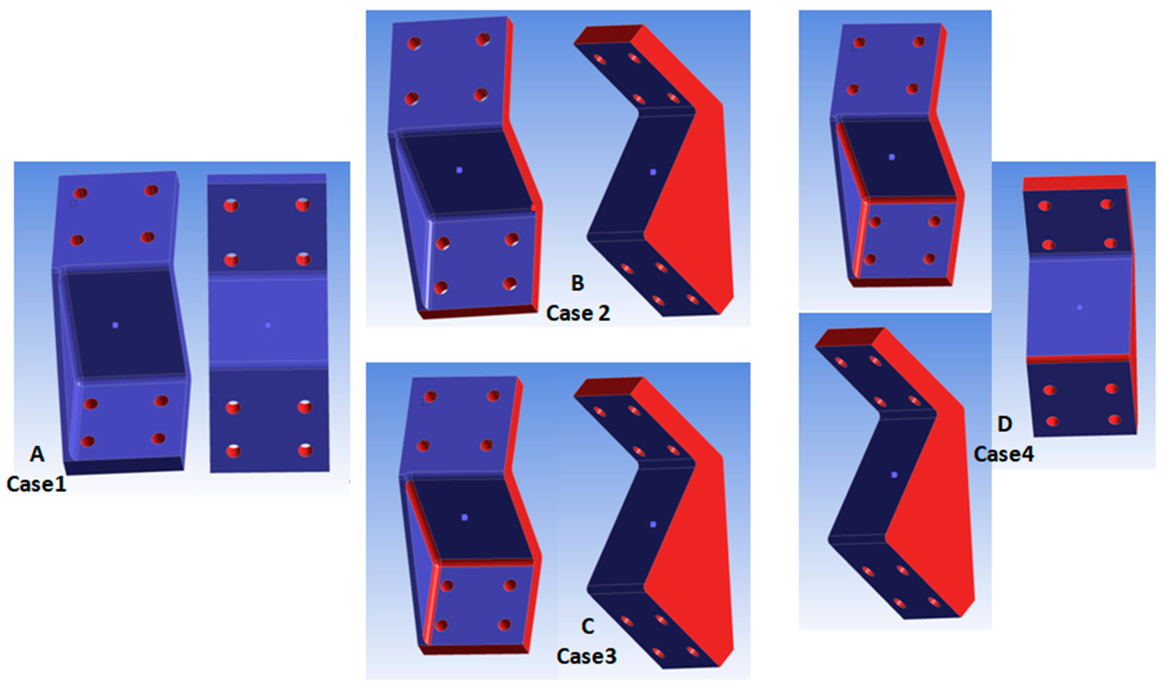
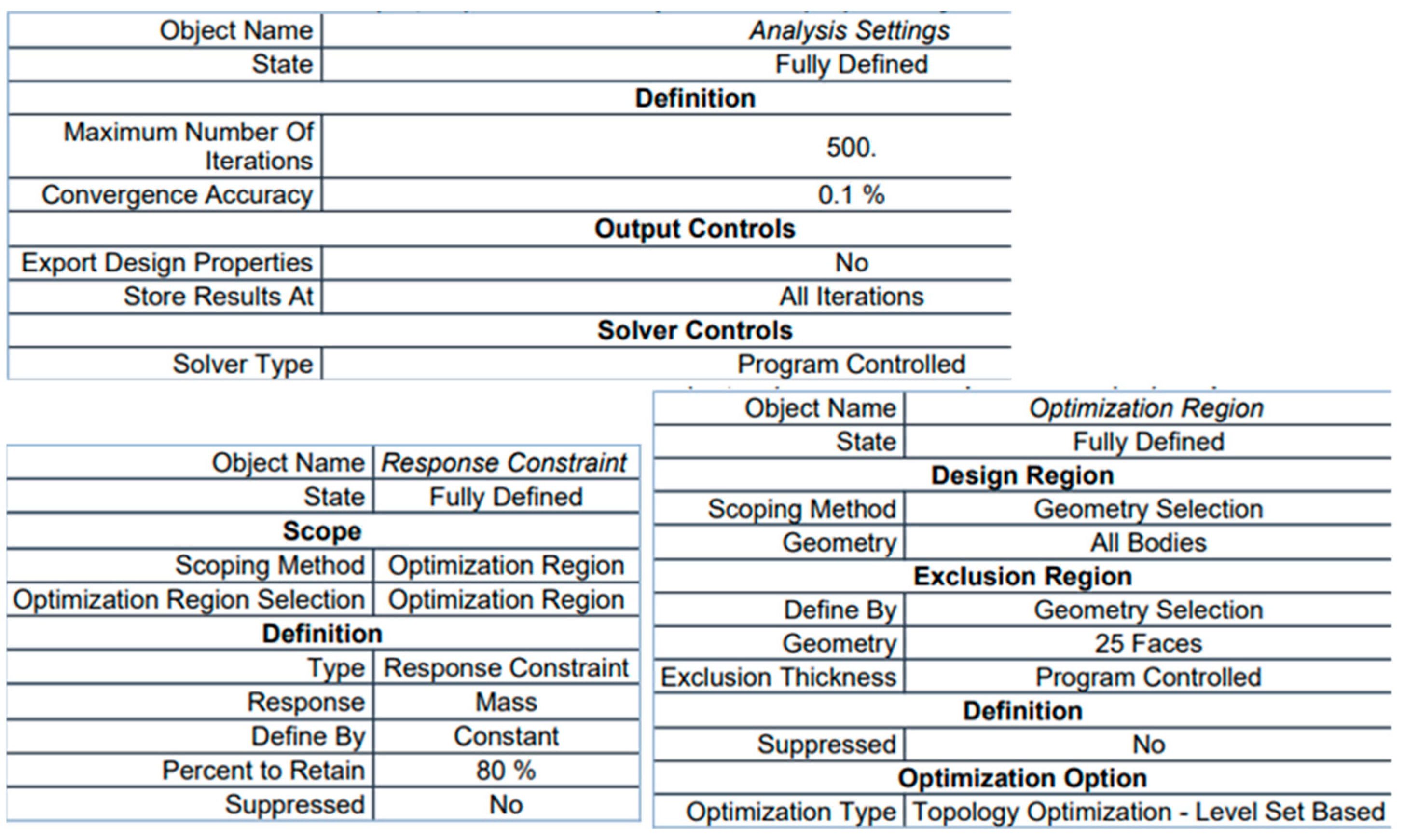
2.1. ANSYS Static Structural Setup for Topology Optimization Analysis

ANSYS Workbench was used as the main platform in our work, orchestrating model setup, structural analysis, and topology optimization, along with all required pre- and post-processing steps, such as mesh generation and refinement, design optimization, and verification. In this work, we aim to minimize compliance, which implies minimizing the strain energy (when only mechanical loads exist) given that lower strain energy leads to increased stiffness. This can be achieved by adding material in regions with higher stress values and removing it from areas that exhibit no or low stress. However, in the studied case, the problem of compliance minimization is considered (equivalently, stiffness maximization) with a given volume fraction constraint, and the additional limitation that the optimized shape cannot lie outside the bracket’s initial surface boundaries. Therefore, the possibility of rearranging material to strengthen weak regions is not considered, but instead, only the reduction of material from areas exhibiting low stresses, with the aim of maintaining the original component’s stiffness.

Within the ANSYS workbench, the Geometry, Static Structural, and Structural Optimization modules were selected and set up. As noted in [28], these modules are needed for performing topology optimization with the methods supported by ANSYS, such as the density-based and the level-set methods. The initial models were modeled in SolidWorks and imported into the workbench through the Geometry Import function, and then transferred to the Static Structural and Structural Optimization modules for meshing, structural analysis, and subsequent topology optimization. After successful mesh generation, analysis, and optimization, the optimized models were transferred back to the Static Structural module for design validation, as described by the protocol used in [29]. These modules are linked in a way that permits information exchange in an iterative manner.

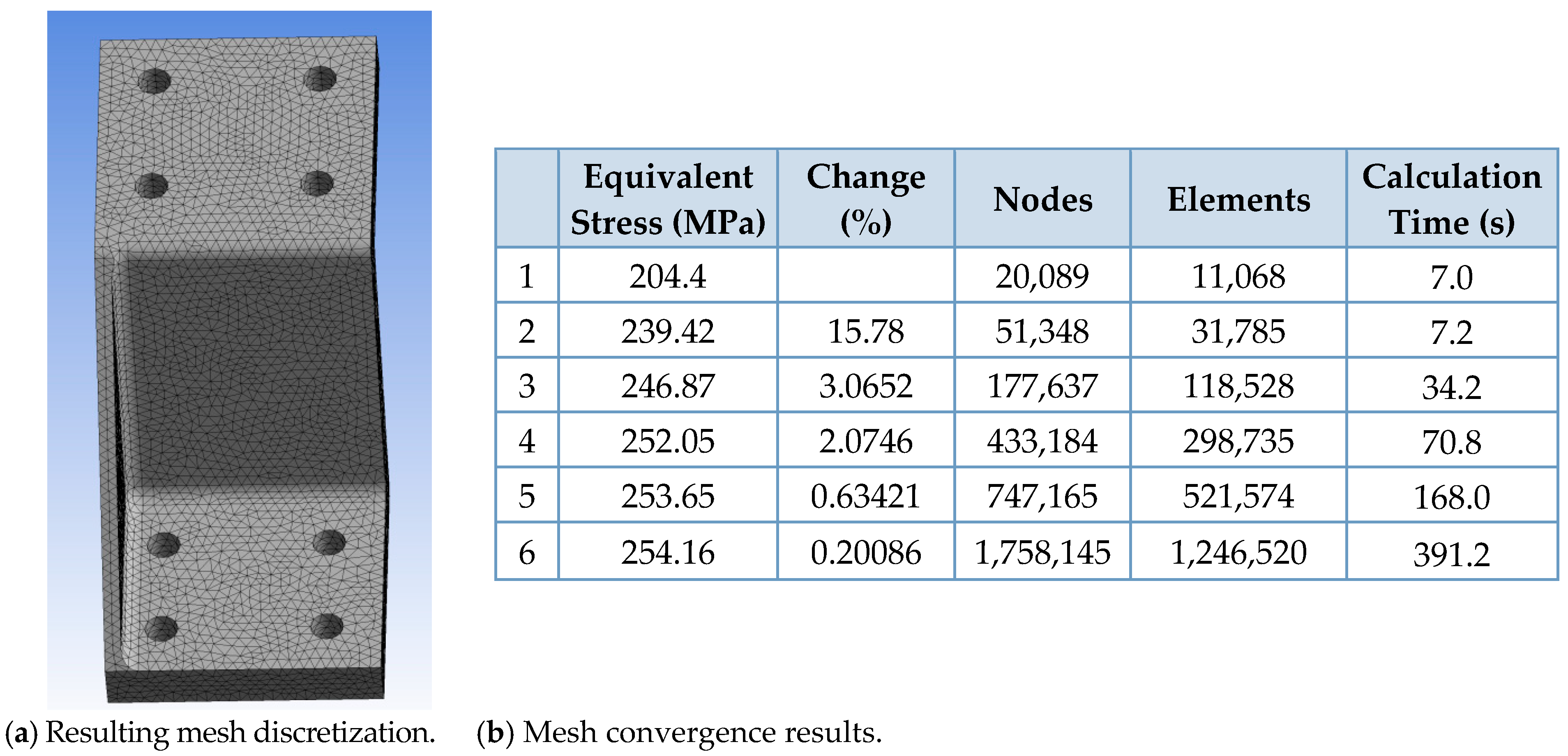
2.2. Mesh Refinement

High quality results can be achieved with relatively lower processing time when appropriate element sizes are selected for a given geometry. The authors in [30] noted that voxelization—which refers to a geometry discretization, when used in topology optimization—decreases the time necessary for iterative analysis of the addition or removal of material from regions where they are either weak or excessively strong. Hence, the mesh was refined by systematically adjusting the mesh settings in ANSYS. The mesh quality was analyzed using the maximum equivalent (von-Mises) stress.

Beginning with the default meshing values, which produced a rather coarse mesh, we performed a mesh convergence study with six levels of refinement to identify an appropriate mesh for the subsequent structural analysis calculations. Successive levels of refinement produced finer meshes relative to the preceding levels. The convergence criteria used in this study were set at <0.5% of allowable change in the equivalent stress of each succeeding refinement level.

For the purpose of this convergence study, structural steel was assumed for the bracket model, having principal dimensions equal to 107.8 × 50 × 67.3 mm, a plate thickness of 10 mm, and a volume of 77,444 mm³, which corresponds to a weight of 0.608 kg when stainless steel is considered. This weight corresponds to approximately 0.059 kg for the unoptimized printed specimen in our study; note that PLA with a printing infill density of 50% was used—see Section 2.4. In Figure 1, image A illustrates the original bracket geometry; B depicts the applied compressive force of 1.5 kN on the bottom face of the bracket; while image C highlights the fixed support applied on the upper face of the bracket (yellow area).

For both the level-set and density-based methods, four optimization scenarios were considered. For case 1, the default option was used for the region to be optimized, which is determined by the boundary conditions only—i.e., the boundary conditions define the region of the design domain that is excluded from the optimization process. For the remaining cases, 2, 3, and 4, we specified the optimization regions using the geometry selection tool, which allows the designer to specify regions to be excluded from the optimization in addition to the ones defined by the boundary conditions. The purpose of cases 2, 3, and 4 was to investigate whether varying the optimization regions would significantly affect the results of the optimized component. The excluded regions for each case are red highlighted in Figure 2, below.

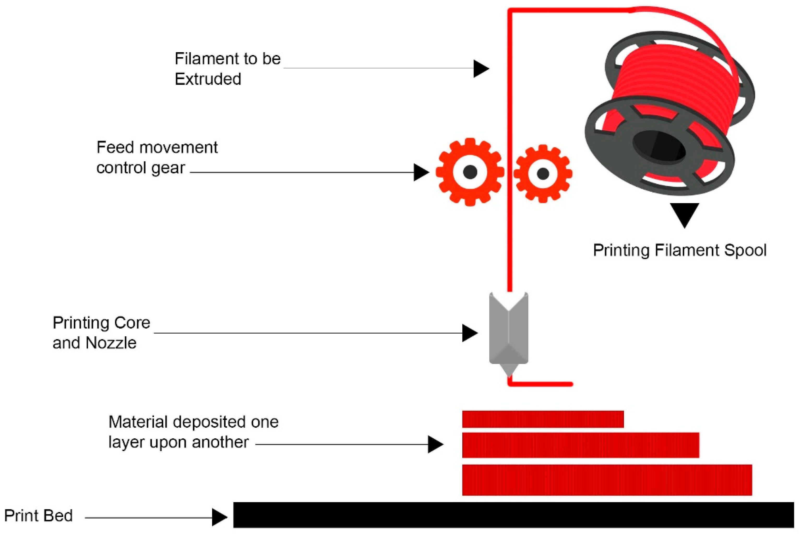
2.3. Fused Deposition Modeling

Fused deposition modeling was used for constructing the prototypes in this work, as it is a readily available technique implemented via low-cost printers and it ensures process simplicity, low operational cost, and relatively higher printing speed using a wide range of available thermoplastics. FDM follows similar processing steps commonly found in several additive manufacturing techniques, i.e., modeling, printing and finishing [31]. Generally, in additive manufacturing, an appropriate software package “slices” CAD data to generate the layers to be printed. The slicer commonly accepts 3D discretizations (triangulations) of solid models commonly described using the stereolithography (STL) format. These discretizations are generated from the solid model using commonly available tools in CAD packages. Depending on the printing setup, the printed object may require post-processing steps, such as surface finishing, support material removal, and sintering.

With the FDM 3D printing technique, polymer filament is used to build components by depositing layer upon layer of polymer through the hot extruder. In this method, the filament is heated to a molten state at the nozzle and afterwards extruded to build successive layers on the build platform [32]; see Figure 3.

2.4. Additive Manufacturing of Parts

After topologically optimizing the bracket, the optimized models were converted into STL files and subsequently sliced using the Ultimaker Cura 5.3.0 software [33]. In the Cura Software, the printing material, printing parameters, and printing conditions were carefully selected according to the desired functionality of the printed part. The printing material used in this work is Ultimaker PLA [34] due to its desirable qualities. According to Ultimaker, PLA (polylactic acid), which is available in 11 colors, is very versatile and easy to use; it is reliable, prints with high dimensional accuracy, and produces surface finish of high quality, thereby making it a good option for different applications such as detailed prototypes, simple manufacturing jigs, and gauges [34]. As noted in relevant literature, the following printing parameters affect the quality of the printed part as well as the total cost of production; hence, they must be carefully selected.

• The printing speed, which defines the material deposition rate and printing time [6,35,36].
• Layer height influences the quality and dimensional accuracy of the printed parts [36,37,38,39,40].
• Extrusion temperature, which is the temperature of the nozzle, affects the viscosity of the melted polymer and so impacts the quality [38,41,42].
• The infill density and its pattern affect the mechanical properties of the FDM 3D-printed part [43].

Based on the studies above [6,35,36,37,38,39,40,41,42,43], the following printing parameter values were selected: printing speed of 65 mm/s, 50% infill density, Triangle infill pattern, and layer height of 0.2 mm. The printing was performed using the Ultimaker (https://ultimaker.com/3d-printers/ultimaker-s5, accessed on 8 September 2023) S5 3D printer, and the recommended temperatures of 60 and 205 °C were set for the build plate and extruder, respectively. After selecting the appropriate printing parameters and slicing the initial and optimized models using the Cura software, the generated printer codes were transferred to the printer where the models were built. In total, 15 samples of the bracket were printed: five for the initial model, and five for each of the level-set and density-based optimized results.

3. Results and Discussion

This section presents and discusses the results of the static structural analysis, topology optimization, and additive manufacturing, as well as the mechanical testing of the 3D-printed parts.

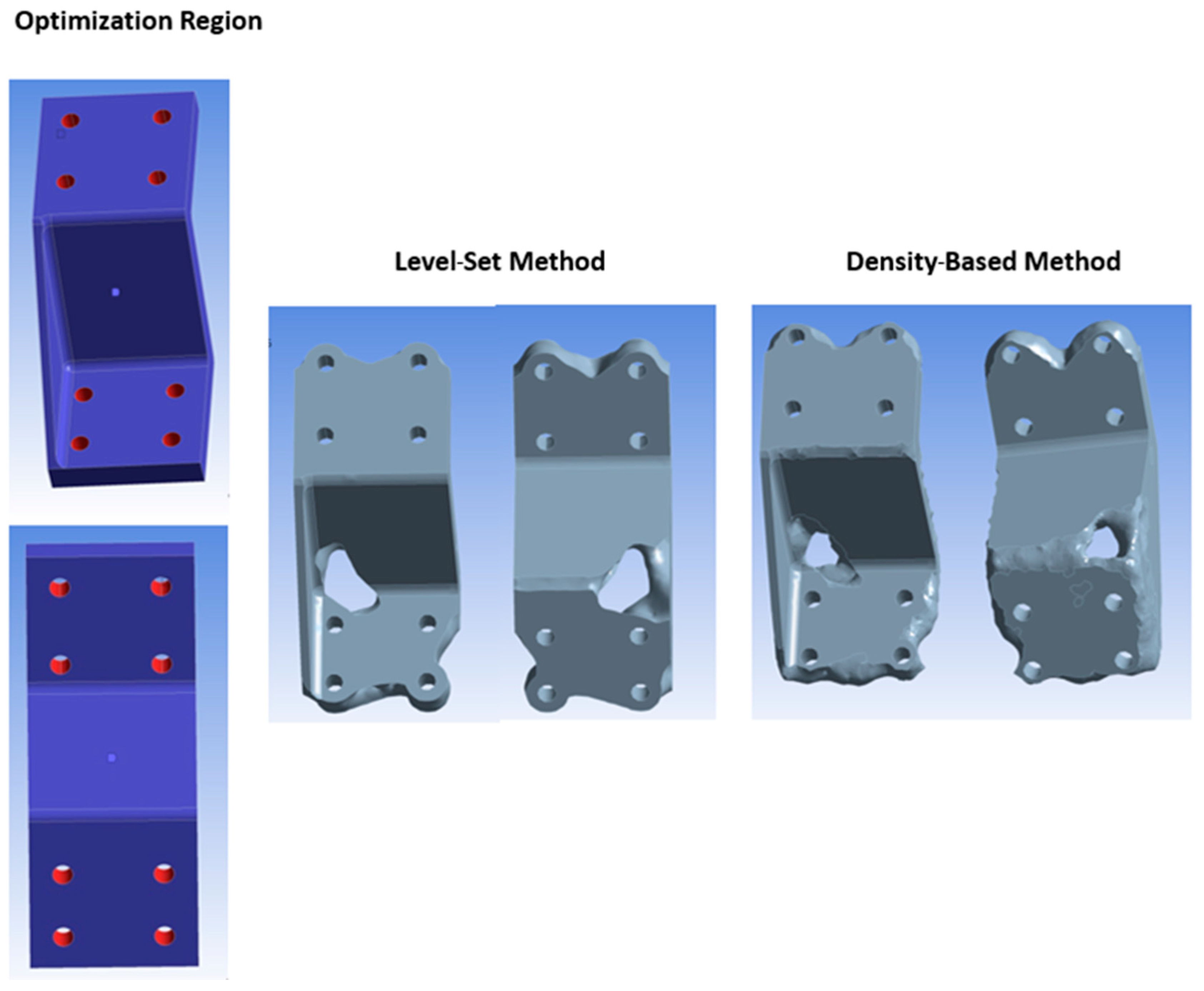
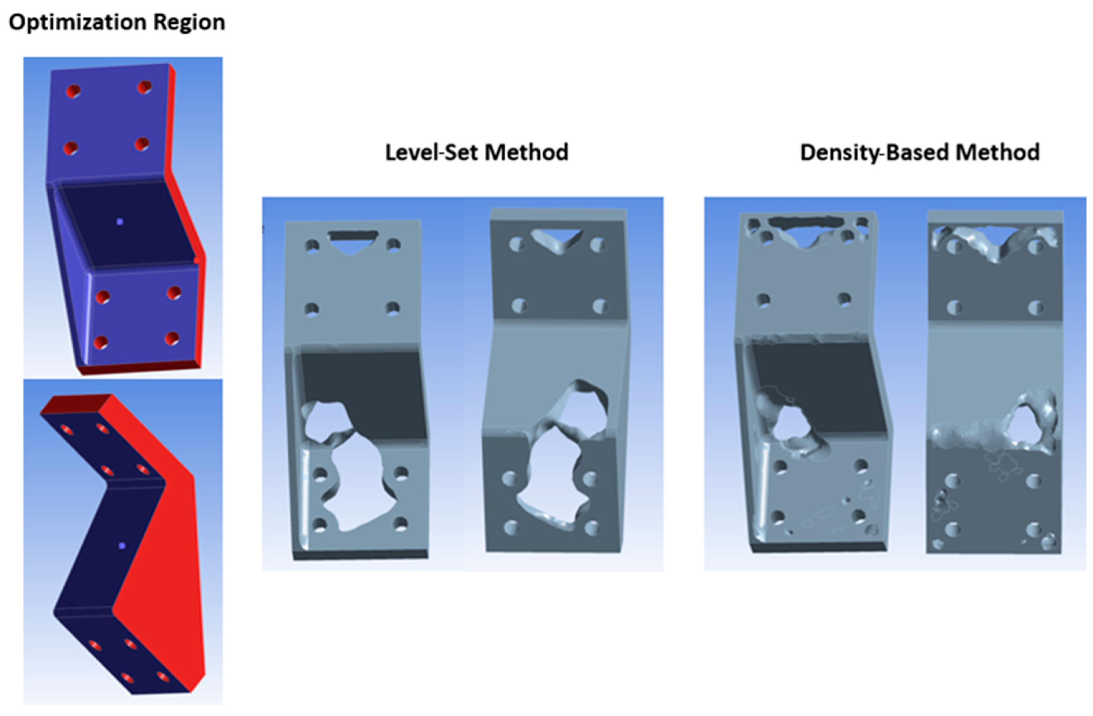
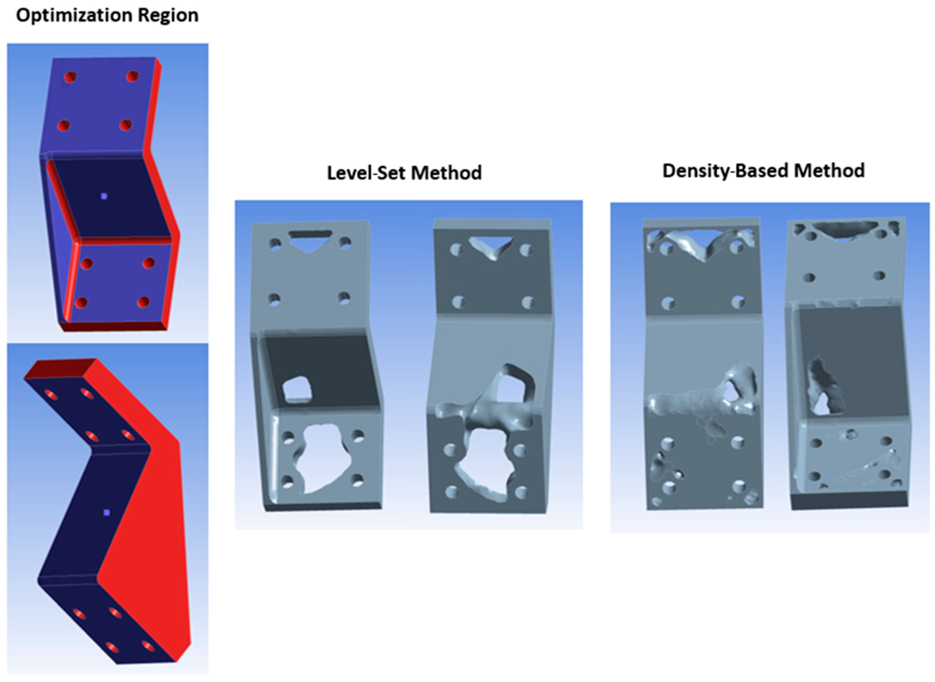
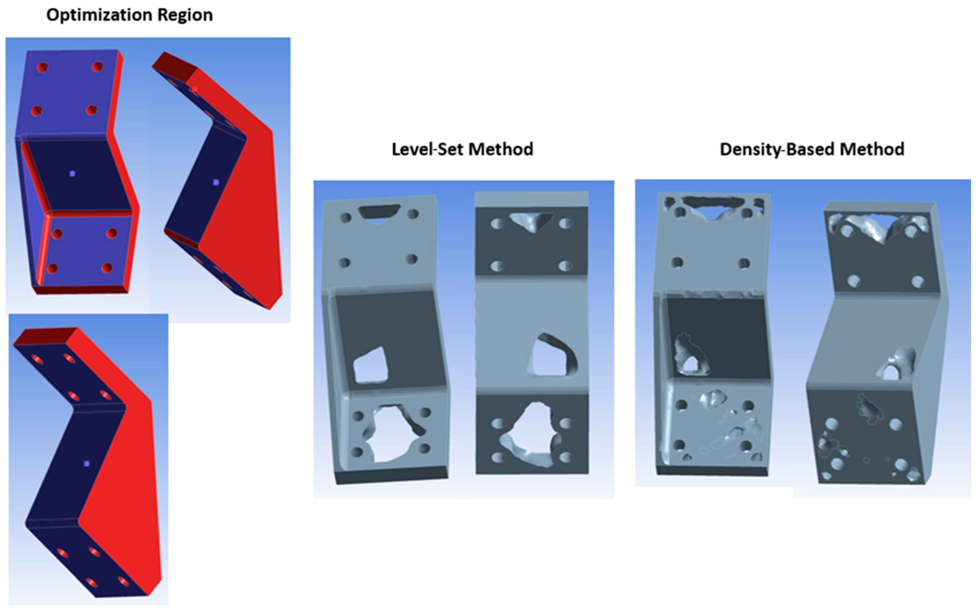
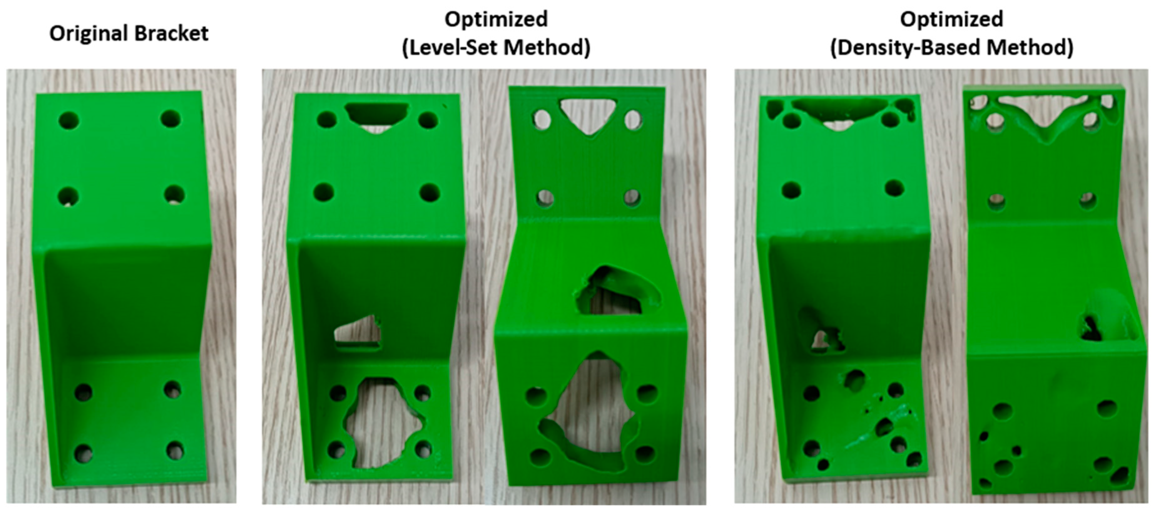
3.1. Optimization Results

The generated mesh with 10-node tetrahedral elements, shown below in Figure 4a, depicts the geometry discretization used for the topology optimization of the bracket. In the same figure, we include the results of the conducted mesh convergence study; see Figure 4b.

From the table in Figure 4b, we observe that the initial setting with an element size (maximum edge length) of 2 mm produced a mesh with 20,089 nodes and 11,068 elements, resulting in 204.4 MPa of equivalent stress. The successive refinement process leads to a converged value of slightly above 250 MPa, while the last refinement in the table has a mesh size of 0.5 mm, with 1,758,145 nodes, 1,246,520 elements, and a value of 254.16 MPa for the equivalent stress. Furthermore, it can be noted from the table that the change in the equivalent stress value between the fourth and fifth meshes is approximately 0.63%, which drops down to 0.2% for the last pair of meshes, indicating mesh convergence. We considered that the fourth level of refinement included in the same table achieves a good balance between computational accuracy and cost, and therefore it was selected for the topology optimization process.

The total deformation and equivalent stress distributions are depicted in Figure 5a and Figure 5b, respectively. The red-colored regions indicate high values, while blue-colored regions correspond to low values.

The topology optimization settings and parameters within the ANSYS package are included in Figure 6, below. A series of material reduction percentages have been considered to evaluate the extent of material reduction, which would maintain similar levels of compliance with the initial design. Specifically, material reductions of 10, 20, 30, and 40% have been attempted, with only the first two percentages yielding compliance levels equal to the original design. Therefore, a material reduction of 20% has been identified as a feasible reduction which would lead to a corresponding weight reduction, from the 0.608 kg of the original design to 0.486 kg for the optimized one (if stainless steel were to be considered in both cases). For the PLA-printed specimens and a 50% infill density, we achieved an actual weight reduction of approximately 19% (from 0.059 kg to 0.048 kg), since wall thickness printing parameters do not allow for a fully homogeneous material distribution. Note that for both level-set and density-based methods, as well as the four cases of optimization domain, the optimization parameters and conditions were the same. A smaller number of specimens (two for each case) were printed and tested with a 100% infill density, but since no significant qualitative difference was observed in the experimental results between the 100% and 50% infill densities, the latter was used. This provides a good basis for the comparison of both methods. The optimized results for both methods and all considered optimization regions are depicted in Figure 7, Figure 8, Figure 9 and Figure 10. From Figure 7, Figure 8, Figure 9 and Figure 10, it is evident that when different regions are considered under the same optimization conditions, different results are obtained through both optimization methods. The exhibited differences between the presented cases is mainly due to the different constrained regions, i.e., red regions where no topology optimization is performed. When the same case is considered, the exhibited differences in the resulting optimized design are mainly due to the employed method; e.g., the level-set method permits a smooth description of the boundary which allows relatively large holes with smooth boundaries to be generated, whereas the SIMP density-based method, with the ANSYS filtering algorithm enabled, generates a large number of holes or deformations on the original design with rough, poorly-defined boundaries.

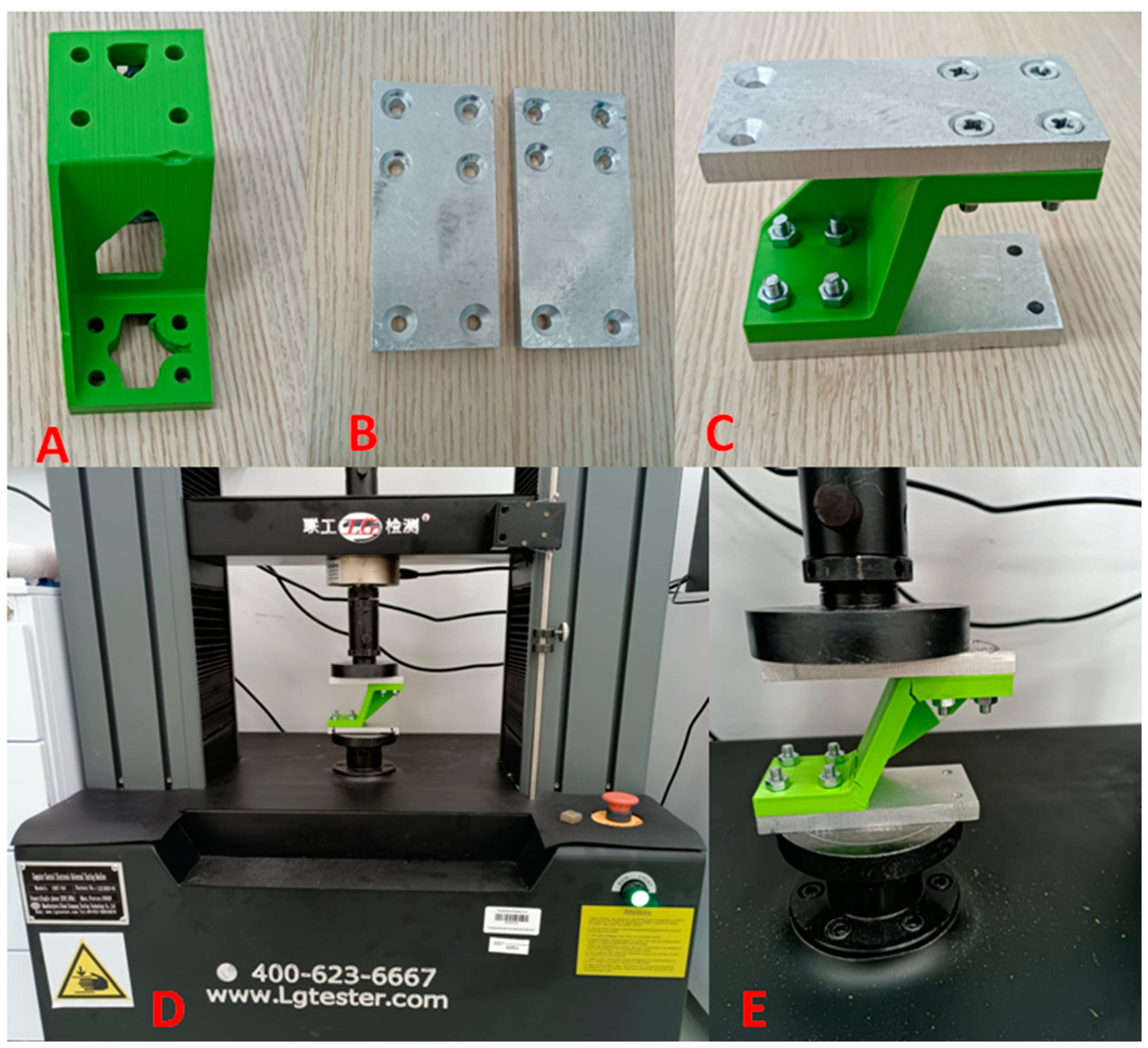
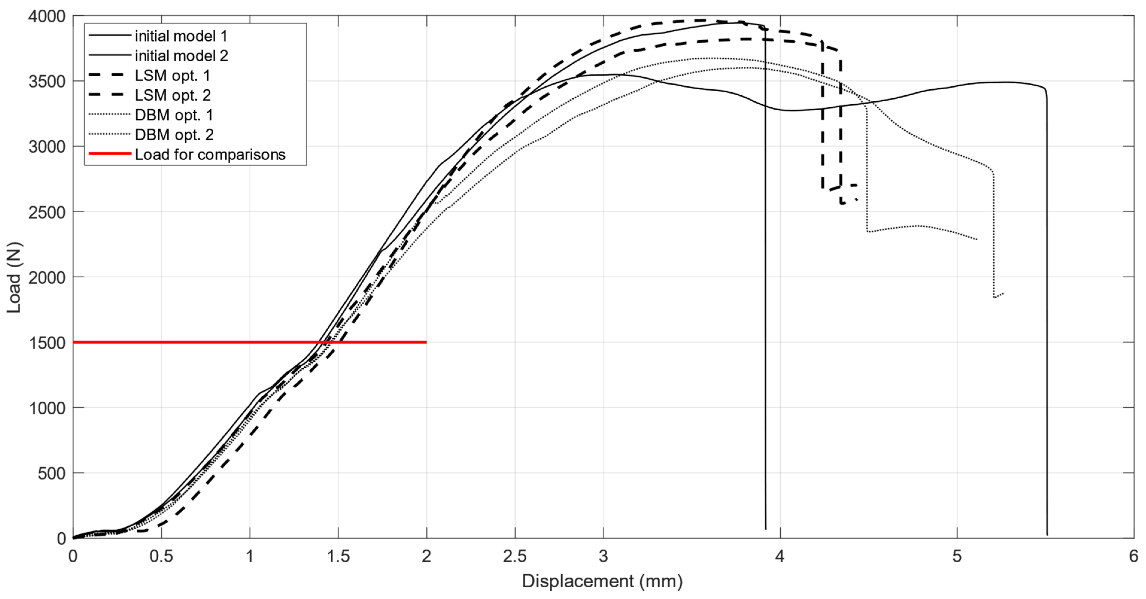
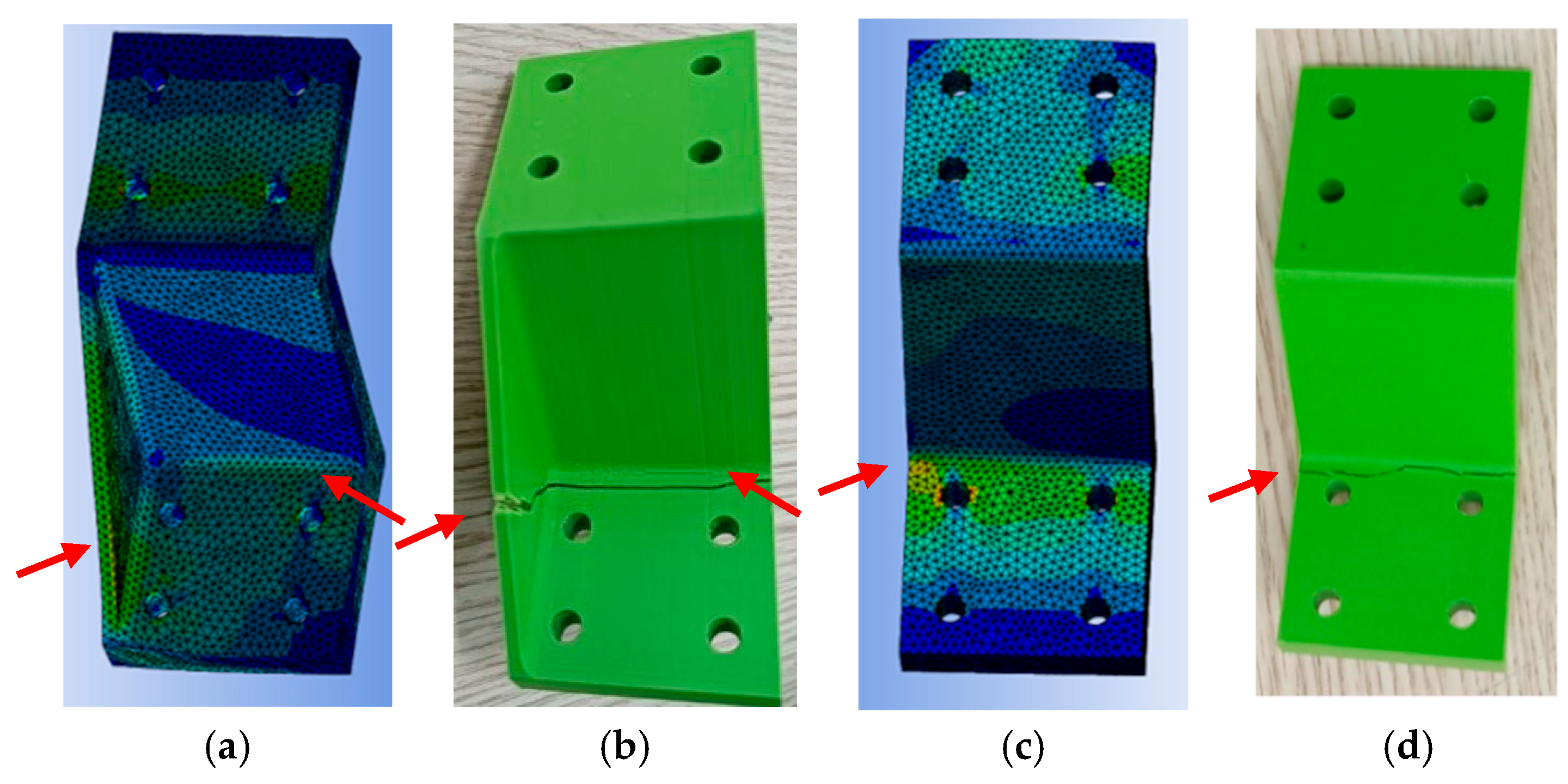
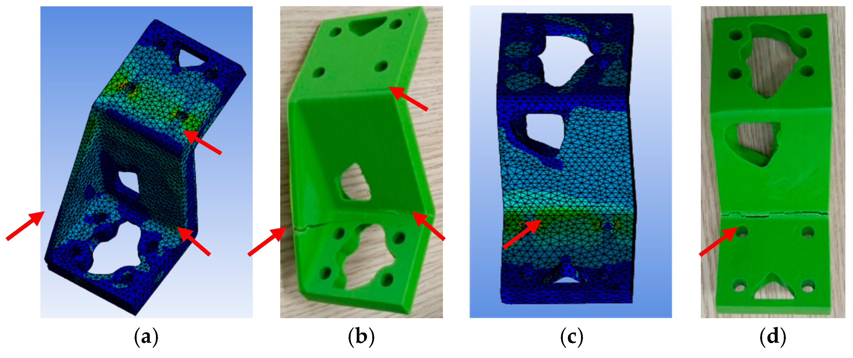
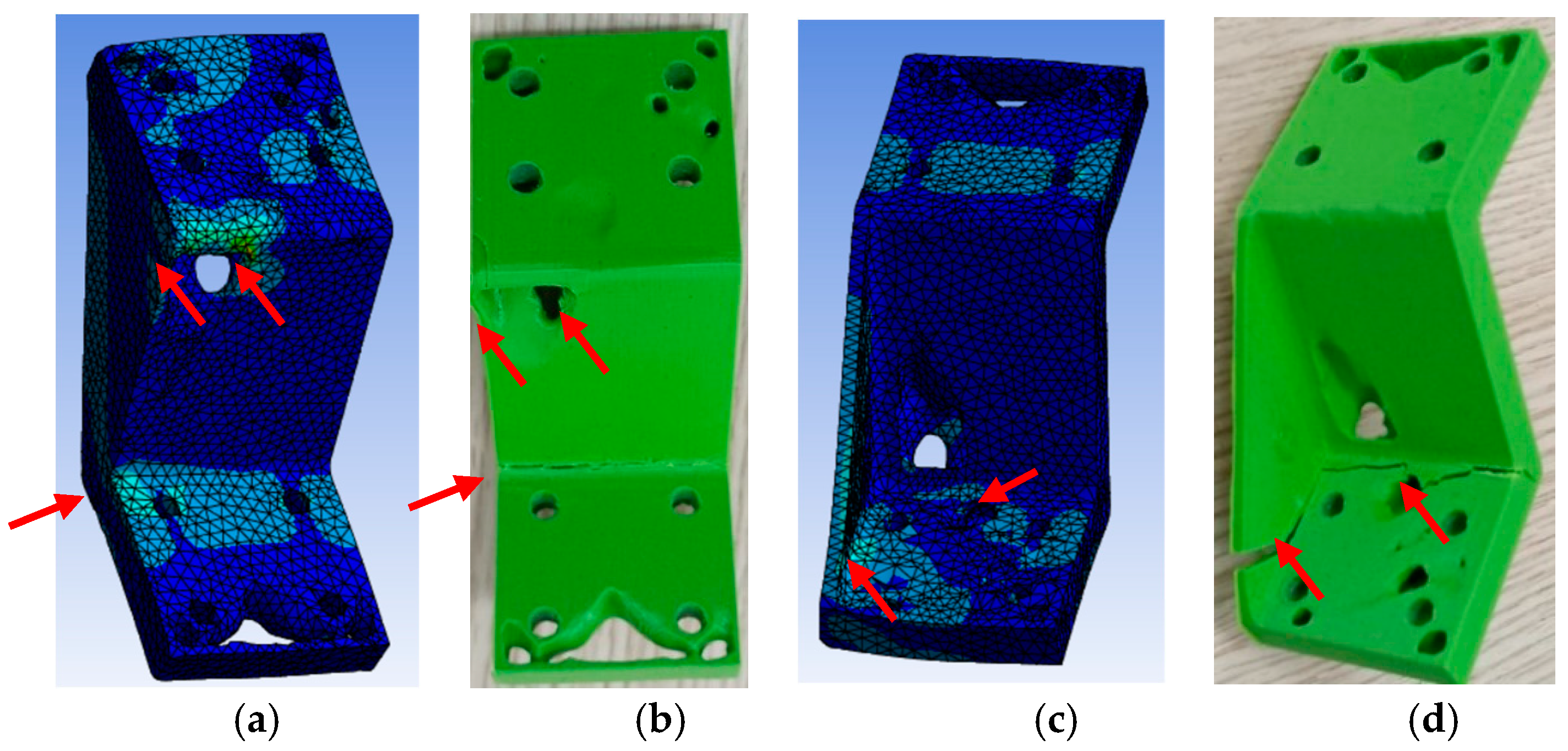
3.2. Experimental Validation

FDM printing was performed for all components to experimentally verify and compare the stiffness of the optimized models (level-set and density-based) to the original one, thus ensuring that they satisfy the objective of material reduction while maintaining approximately the same displacement levels exhibited by the unoptimized model. As mentioned previously, the 3D printing of the bracket was done using the Ultimaker 3D printer, with the Ultimaker PLA as the printing material and the analysis being adapted to the same material. For this experiment, only cases 3 and 4 of the optimized models were considered as they achieved, in the analysis phase, displacement results matching those of the original model. Figure 11 shows the printed unoptimized (original) and optimized parts of the bracket for the two methods in both cases (3 and 4).

Five replicates of the original bracket design and ten optimized design replicates were printed and tested (five for the level-set method and five for the density-based method). The initial and optimized specimens were printed under the same printing conditions to ensure comparability and accuracy of the results. We also arranged the placement of printed components in a way that would yield the same printing orientation, as well as printing without overhangs, to eliminate the need for support material and post-processing which could potentially differentiate the properties of the printed specimens. The LG SmartTester compression machine (http://www.lgtester.com/English/index.php?m=content&c=index&a=lists&catid=16, accessed on 8 September 2023) was used for testing displacements (stiffness) under the same loading conditions (a compressive load of 1.5 kN). Custom testing fixtures were fabricated to ensure the placement and loading conditions for all tested specimens and secure them in place; Figure 12 depicts the setup for the corresponding compressive testing. As can be seen in Figure 12, A corresponds to the 3D-printed bracket; B is the employed fixture, designed to secure the bracket in place and ensure the same testing conditions; while C depicts the bracket–fixture assembly. Finally, Figure 12D shows the component in testing position, with E capturing a snapshot of a bracket specimen undergoing fracture under a compressive force.

The results for the five tested replicates are shown in

Table 1. Displacement (mm) of tested specimens under a 1.5 kN compressive load.

Nr.	Original	Optimized (LSM)	Optimized (DBM)
1	1.25	1.47	1.9
2	1.39	1.44	1.47
3	1.46	1.51	1.46
4	1.71	1.44	1.56
5	1.42	1.49	1.43
Mean	1.45	1.47	1.56
Std. Dev.	0.150	0.028	0.174

. Only two specimens (out of five for each design) are shown in Figure 13 for the sake of clarity, and it is easy to see that the LSM-optimized design is more in alignment with the behavior of the initial unoptimized design.

As mentioned previously, to ensure the accuracy of the results, both the original and optimized models were placed and secured in the exact same positions when applying the compressive loads. From these results (see Table 1), under the same load of 1.5 kN and the exact same printing and testing conditions, the mean displacement values were 1.45, 1.47, and 1.56 mm for the initial, LSM-optimized, and DBM-optimized designs, respectively. The mean values, along with the reported standard deviations, indicate the achievement of the topology optimization objective for both methods, although the level-set method seems to produce more consistent results, with a better match to the displacement of the unoptimized design. Finally, a comparison between the regions of failure and the high stress regions of the initial model and the two optimized models in case 4 are depicted in Figure 14, Figure 15 and Figure 16. As one may easily observe by following the red arrows on these figures, the regions of failure are in alignment with the high stress concentration regions identified in the analysis.

4. Conclusions

The integration of topology optimization into additive manufacturing for a practical bracket-design case has been successfully demonstrated with the analysis results experimentally validated under compressive loading. Two of the most common methods in topology optimization, particularly the level-set and density-based methods, were compared numerically and experimentally, and it was found that the level-set method showed more consistent results with respect to the analysis-predicted compliance levels, and a better match to the initial design’s performance. Additionally, a study related to the appropriate identification of the regions selected for optimization was conducted, as the default method selections may not necessarily yield the desired results. Based on the results obtained, it was demonstrated that by selecting the appropriate discretization and optimization regions, we can produce consistent results with a 20% weight/material reduction while maintaining the stiffness performance of the initial design. Overall, the optimized components compete favorably with the original model, with a negligible difference in the mean deformation, especially for the level-set method.

As indicated in this study, the selection of regions for topology optimization greatly affects the achieved designs, and future studies need to be carried out to improve the ability of the topology optimization models to automatically identify the optimization regions, which would result in better and more consistent results.

References

1. Society of Manufacturing Engineers and SME. Additive Manufacturing Glossary. Available online: https://www.sme.org/technologies/additive-manufacturing-glossary/ (accessed on 22 November 2022).
2. Joshi, S.C.; Sheikh, A.A. 3D printing in aerospace and its long-term sustainability. Virtual Phys. Prototyp. 2015, 10, 175–185. [Google Scholar] [CrossRef]
3. ASTM F2792-12a; Standard Terminology for Additive Manufacturing Technologies. ASTM International: West Conshohocken, PA, USA, 2012.
4. Ali, M.H.; Batai, S.; Sarbassov, D. 3D printing: A critical review of current development and future prospects. Rapid Prototyp. J. 2019, 25, 1108–1126. [Google Scholar] [CrossRef]
5. Diegel, O.; Kristav, P.; Motte, D.; Kianian, B. Additive manufacturing and its effect on sustainable design. In Environmental Footprints and Eco-Design of Products and Processes; SGS Hong Kong Limited: Hong Kong, China, 2016. [Google Scholar] [CrossRef]
6. Bhuvanesh, M.K.; Sathiya, P. Methods and materials for additive manufacturing: A critical review on advancements and challenges. Thin-Walled Struct. 2021, 159, 107228. [Google Scholar] [CrossRef]
7. Thomas, D. Costs, benefits, and adoption of additive manufacturing: A supply chain perspective. Int. J. Adv. Manuf. Technol. 2016, 85, 1857–1876. [Google Scholar] [CrossRef] [PubMed]
8. Pérez, M.; Carou, D.; Rubio, E.M.; Teti, R. Current advances in additive manufacturing. Procedia CIRP 2020, 88, 439–444. [Google Scholar] [CrossRef]
9. Sabiston, G.; Kim, I.Y. 3D topology optimization for cost and time minimization in additive manufacturing. Struct. Multidiscip. Optim. 2020, 61, 731–748. [Google Scholar] [CrossRef]
10. Kazybek, K.; Konstantinos, K.; Didier, T. Topology Optimization for Additive Manufacturing. In Proceedings of the EUSPEN, Advancing Precision in Additive Manufacturing, Virtual, 21–23 September 2021; EUSPEN: St. Gallen, Switzerland, 2021. Available online: https://www.euspen.eu/events/sig-meeting-additive-manufacturing-2021/?subid=sig-meeting-additive-manufacturing-2021 (accessed on 8 September 2023).
11. Formlabs, Topology Optimization 101: How to Use Algorithmic Models to Create Lightweight Design. Available online: https://formlabs.com/blog/topology-optimization/ (accessed on 8 September 2023).
12. Prathyusha, A.L.R.; Raghu Babu, G. A review on additive manufacturing and topology optimization process for weight reduction studies in various industrial applications. Mater. Today Proc. 2022, 62, 109–117. [Google Scholar] [CrossRef]
13. Zhu, J.; Zhou, H.; Wang, C.; Zhou, L.; Yuan, S.; Zhang, W. A review of topology optimization for additive manufacturing: Status and challenges. Chin. J. Aeronaut. 2021, 34, 91–110. [Google Scholar] [CrossRef]
14. Querin, O.M.; Victoria, M.; Alonso, C.; Ansola, R.; Martí, P. Topology Design Methods for Structural Optimization; Butterworth-Heinemann: Oxford, UK, 2017. [Google Scholar]
15. Dems, K. First- and second-order shape sensitivity analysis of structures. Struct. Optim. 1991, 3, 79–88. [Google Scholar] [CrossRef]
16. Sigmund, O.; Maute, K. Topology optimization approaches: A comparative review. Struct. Multidiscip. Optim. 2013, 48, 1031–1055. [Google Scholar] [CrossRef]
17. Bendsøe, M.P.; Kikuchi, N. Generating optimal topologies in structural design using a homogenization method. Comput. Methods Appl. Mech. Eng. 1988, 71, 197–224. [Google Scholar] [CrossRef]
18. Bendsøe, M.P. Optimal shape design as a material distribution problem. Struct. Optim. 1989, 1, 193–202. [Google Scholar] [CrossRef]
19. Van Dijk, N.P.; Langelaar, M.; van Keulen, F. Critical Study of Design Parametrization in Topology Optimization: The influence of design parametrization on local minima. In Proceedings of the 2nd International Conference on Engineering Optimization, Lisbon, Portugal, 6–9 September 2010. [Google Scholar]
20. Van Dijk, N.P.; Maute, K.; Langelaar, M.; Van Keulen, F. Level-set methods for structural topology optimization: A review. Struct. Multidiscip. Optim. 2013, 48, 437–472. [Google Scholar] [CrossRef]
21. Wang, M.Y.; Wang, X.; Guo, D. A level set method for structural topology optimization. Comput. Methods Appl. Mech. Eng. 2003, 192, 227–246. [Google Scholar] [CrossRef]
22. Allaire, G.; Jouve, F.; Toader, A.M. Structural optimization using sensitivity analysis and a level-set method. J. Comput. Phys. 2004, 194, 363–393. [Google Scholar] [CrossRef]
23. Osher, S.; Sethian, J.A. Fronts propagating with curvature-dependent speed: Algorithms based on Hamilton-Jacobi formulations. J. Comput. Phys. 1988, 79, 12–49. [Google Scholar] [CrossRef]
24. Bendsøe, M.P.; Sigmund, O. Optimization of Structural and Mechanical Systems; World Scientific: Singapore, 2007. [Google Scholar]
25. Huang, X.; Xie, Y.M. A further review of ESO type methods for topology optimization. Struct. Multidiscip. Optim. 2010, 41, 671–683. [Google Scholar] [CrossRef]
26. Dunning, P.D.; Kim, H.A. Introducing the sequential linear programming level-set method for topology optimization. Struct. Multidiscip. Optim. 2015, 51, 631–643. [Google Scholar] [CrossRef]
27. Haveroth, G.A.; Thore, C.J.; Correa, M.R.; Ausas, R.F.; Jakobsson, S.; Cuminato, J.A.; Klarbring, A. Topology optimization including a model of the layer-by-layer additive manufacturing process. Comput. Methods Appl. Mech. Eng. 2022, 398, 115203. [Google Scholar] [CrossRef]
28. Lee, H.H. Finite Element Simulations with ANSYS Workbench 18; SDC Publications: Mission, KA, USA, 2018. [Google Scholar]
29. Thompson, M.K.; Thompson, J.M. ANSYS Mechanical APDL for Finite Element Analysis; Butterworth-Heinemann: Oxford, UK, 2017. [Google Scholar]
30. Bacciaglia, A.; Ceruti, A.; Liverani, A. A systematic review of voxelization method in additive manufacturing. Mech. Ind. 2019, 20, 630. [Google Scholar] [CrossRef]
31. Bhatnagar, A.; Bhardwaj, A.; Verma, S. Additive Manufacturing: A 3-Dimensional Approach in Periodontics. J. Adv. Med. Med. Res. 2020, 32, 105–117. [Google Scholar] [CrossRef]
32. Rouf, S.; Malik, A.; Singh, N.; Raina, A.; Naveed, N.; Siddiqui, M.I.H.; Haq, M.I.U. Additive manufacturing technologies: Industrial and medical applications. Sustain. Oper. Comput. 2022, 3, 258–274. [Google Scholar] [CrossRef]
33. Ultimaker. UltiMaker Cura 5.3.0. Available online: https://github.com/Ultimaker/Cura/releases/tag/5.3.0-beta.1 (accessed on 8 September 2023).
34. Ultimaker. Ultimaker Material, PLA. Available online: https://ultimaker.com/materials/pla (accessed on 8 September 2023).
35. Rayegani, F.; Onwubolu, G.C. Fused deposition modelling (fdm) process parameter prediction and optimization using group method for data handling (gmdh) and differential evolution (de). Int. J. Adv. Manuf. Technol. 2014, 73, 509–519. [Google Scholar] [CrossRef]
36. Galetto, M.; Verna, E.; Genta, G. Effect of process parameters on parts quality and process efficiency of fused deposition modeling. Comput. Ind. Eng. 2021, 156, 107238. [Google Scholar] [CrossRef]
37. UKEssays. Principles of Additive Manufacturing. Available online: https://www.ukessays.com/essays/engineering/principles-of-additive-manufacturing-engineering-essay.php?vref=1 (accessed on 8 September 2023).
38. Sood, A.K.; Ohdar, R.K.; Mahapatra, S.S. Improving dimensional accuracy of Fused Deposition Modelling processed part using grey Taguchi method. Mater. Des. 2009, 30, 4243–4252. [Google Scholar] [CrossRef]
39. Nuţă, A.B.; Ulmeanu, M.E.; Doicin, C.V. Design for 3D Printing: Case study for a cold plastic deformation mould. MATEC Web Conf. 2021, 343, 04008. [Google Scholar] [CrossRef]
40. 3D Hubs. The Impact of Layer Height on a 3D Print. Available online: https://www.3dhubs.com/knowledge-base/impact-layer-height-3d-print/ (accessed on 8 September 2023).
41. Luzanin, O.; Guduric, V.; Ristic, I.; Muhic, S. Investigating impact of five build parameters on the maximum flexural force in FDM specimens—A definitive screening design approach. Rapid Prototyp. J. 2017, 23, 1088–1098. [Google Scholar] [CrossRef]
42. Solomon, I.J.; Sevvel, P.; Gunasekaran, J. A review on the various processing parameters in FDM. Mater. Today Proc. 2020, 37, 509–514. [Google Scholar] [CrossRef]
43. Alafaghani, A.; Qattawi, A. Investigating the effect of fused deposition modeling processing parameters using Taguchi design of experiment method. J. Manuf. Process. 2018, 36, 164–174. [Google Scholar] [CrossRef]
Figure 1. Boundary conditions for analysis; (A): bracket model, (B): force application, and (C): additional boundary conditions.
Applsci 13 13218 g001
Figure 2. Domain regions for optimization (blue) along with the excluded regions (red) for the four studied scenarios.
Applsci 13 13218 g002
Figure 3. Typical FFF Printing.
Applsci 13 13218 g003
Figure 4. Resulting mesh and mesh convergence study.
Applsci 13 13218 g004
Figure 5. (a) Total deformation; (b) equivalent stress.
Applsci 13 13218 g005
Figure 6. Topology optimization settings, as defined in ANSYS.
Applsci 13 13218 g006
Figure 7. Optimization region of Case 1.
Applsci 13 13218 g007
Figure 8. Optimization region of Case 2.
Applsci 13 13218 g008
Figure 9. Optimization region of Case 3.
Applsci 13 13218 g009
Figure 10. Optimization region of Case 4.
Applsci 13 13218 g010
Figure 11. 3D-printed components (original, optimized through level-set method, and optimized through density-based method).
Applsci 13 13218 g011
Figure 12. Setup for mechanical testing; (A): printed component, (B): fixture, (C): component/fixture assembly, (D): component under compressive test, (E): component failure.
Applsci 13 13218 g012
Figure 13. The indicative load–displacement curves for two specimens corresponding to each design: initial bracket model (solid lines), design optimized with the level-set method (dashed lines), and density-based optimization design (thin dotted line); the red straight line corresponds to the load used for comparisons in Table 1.
Applsci 13 13218 g013
Figure 14. Comparison of the regions of failure with the corresponding regions of high-stress concentration in the analysis of the initial unoptimized bracket. (a,c) depict the estimated stress distribution with (b,d) depicting the failure locations on the tested components; red arrows indicate the correspondence between high-stress and failure regions.
Applsci 13 13218 g014
Figure 15. Comparison of the regions of failure with the corresponding regions of high-stress concentration in the analysis of the level-set optimized bracket (case 4). (a,c) depict the estimated stress distribution with (b,d) depicting the failure locations on the tested components; red arrows indicate the correspondence between high-stress and failure regions.
Applsci 13 13218 g015
Figure 16. Comparison of the regions of failure with the corresponding regions of high-stress concentration in the analysis of the density-based optimized bracket (case 4). (a,c) depict the estimated stress distribution with (b,d) depicting the failure locations on the tested components; red arrows indicate the correspondence between high-stress and failure regions.
Applsci 13 13218 g016