Mathematical Modeling of Groundwater Flow: A Case Study of Foundation Piles in the Vicinity of Danube River

Abstract

This study investigated the interaction of groundwater flow and foundation piles located in the vicinity of the Danube River. The piles represent an obstacle to the groundwater flow, causing a backwater effect upstream whilst increasing the local flow velocity. On the other hand, a high flow velocity around the piles can cause suffusion of the surrounding soil in the long term, thus significantly reducing the shaft resistance of the piles. A 3D model of groundwater flow and its impact on the piles was developed in the software 10.3 package GMS based on MODFLOW 2005. The model was calibrated by comparing the calculated results with the measured values in the control well for different values of the filtration coefficients. In the calibration process, foundation piles were not applied in the model. After the calibration process, the piles were implemented into the model and the underground flow was simulated in the study area for the calibrated year 2006. The impact analysis was carried out by comparing the groundwater level change over time in the pile zone at three control points, in cases with and without the piles, along with the flow net analysis at the piles’ location. The results indicate no influence of the piles on the groundwater flow in the study area, both in terms of critical flow velocities and a possible backwater effect upstream.

1. Introduction

Groundwater represents the third most abundant component in the global water cycle, along with oceans and snow (glaciers). Groundwater and glaciers comprise more than 97% of all fresh water on earth [1]. Moreover, they are two of the most important sources of drinking water, used for many different purposes such as agriculture, industry, water supply to the population, etc. [2,3,4]. Groundwater research has been gaining importance in recent years due to the growing awareness of the need for groundwater, as well as the increasing decline in its quality and quantity. The numerous issues that have arisen during groundwater research, such as forecasting groundwater level and, consequently, determining the aquifer thickness, have led to the development of various simulation models which describe and predict the groundwater flow [5].

Numerical modeling is a powerful tool that serves to provide a better comprehension of groundwater flow and to obtain information about important groundwater parameters. The most important aspect of the use of such models is acquiring data on the real conditions occurring within the observed environment. Namely, such models provide sufficient information for the efficient management of groundwater resources [6,7,8,9,10]. The first step in the modeling process is creating a conceptual model. In the next step, this conceptual model is converted into appropriate mathematical expressions which are combined with boundary conditions to form a mathematical model. Although these models are quite complex and characterized by a large amount of input data, their application is extensive. One of the most commonly used numerical modeling software is GMS based on MODFLOW 2005, developed by Aquaveo, LLC in Provo, Utah, USA [11].

A number of authors have used MODFLOW in groundwater modeling for various purposes. Some of them combined it with other models and software for more reliable research results. For example, in [12], the groundwater level was estimated using three models: MODFLOW, ELM, and WA-ELM. Based on the obtained numerical results from all three models, WA-ELM was proven to be a superior model for groundwater level simulation. Fioreze and Mancuso [13] analyzed constructed wetlands as alternatives for decentralized wastewater treatment. They used MODFLOW and MODPATH software included in Groundwater Modeling System (GMS) version 9.0.3, based on the finite difference method, to simulate flow in wetlands numerically. The model has proven to be a powerful tool for 3D simulation, allowing the representation of flow distributions, velocities, elevations, and particle trajectories. Almuhaylan et al. [14] analyzed arid regions characterized by groundwater withdrawal. They applied a three-dimensional finite difference model (MODFLOW) to a unique aquifer to assess the impact of different groundwater pumping scenarios on aquifer depletion. The study showed that the existing pumping rates could lead to an alarming drop in the groundwater level. Furthermore, Visual-MODFLOW 2000 was utilized for groundwater level analysis in the Purba Midnapur area (West Bengal, India) in [15]. The study was designed to predict the groundwater level in the future usage scenarios for the purposes of better groundwater management. Licata et al. [16] conducted a hydrogeological study to find out the cause of groundwater flooding. The flow model was calibrated for steady and unsteady state using the automatic calibration code, Model-Independent Parameter Estimation (PEST). To evaluate the Jilin urban area’s groundwater resources and aquifer system (JUA, Jilin province in northeast China), Qiu et al. [17] established a numerical groundwater flow model using GMS based on data from 190 boreholes. Recharge proved to be the most sensitive factor in this model. Based on the supply and demand analysis of water resources, the developed model could finally provide a scientific basis for using groundwater resources sustainably in JUA. The objective of [18] was to model the Birjand aquifer (Eastern Iran) using GMS: MODFLOW to monitor the groundwater status in the Birjand region. The model’s results agreed with the observed data; therefore, the model could be used to study the changes in the aquifer’s water level. Wondzell et al. [19] addressed the questions of how reliable hyporheic groundwater models are in typical applications examining such flow exchanges, and how reliability changes with increased data availability and model sophistication. The increased model sophistication was shown not to lead to improved model reliability as the travel time predictions from the homogeneous model were equal to, or better than, the predictions from the heterogeneous models. Li et al. [20] analyzed the connection between shallow groundwater and vegetation growth, which is generally very close. The first conclusion was that the water table and salinity are the main factors controlling shallow groundwater. Secondly, regulation plans for the water table and salinity were designed based on the corresponding regulation target. Finally, the output results from the software could provide information on how to regulate shallow groundwater in different scenarios. Various studies deal with the effects piles have on groundwater and their mutual interaction. For example, in [21], pile stability due to rising groundwater levels was evaluated to propose preliminary guidelines to protect existing structures. The results showed that groundwater rises caused upward movement of the ground and the pile foundation. It also caused a loss in pile foundation capacity. As a result of the soil swelling around the pile, the pile shaft friction was reduced. The same authors in another study [22] used a numerical model to investigate pile behavior due to the rising groundwater level. The pile–soil movement, load the distribution along the pile, and the reduction in pile capacity were observed. Besides the fact that the pile load capacity was again significantly reduced by the increase in the groundwater level, it was concluded that the pile foundation showed less heave than the surrounding soil surface during the groundwater level rising. Yuan et al. [23] analyzed the influence of the groundwater level and cyclic load magnitude on the performance of the pile–soil system, introducing the fractal theory. It was shown that the fractal dimension could reflect the load response of the pile–soil system under cyclic loading.

This study’s primary goal was to gain insight into the interaction of groundwater flow and foundation piles near a river using a 3D numerical model described below. The findings suggest that the piles represent an obstacle to the groundwater flow, causing a backwater effect upstream while increasing the local flow velocity. On the other hand, a high flow velocity around the piles can cause the suffusion of the surrounding soil in the long term, thus significantly reducing the shaft resistance of the piles.

2. Materials and Methods

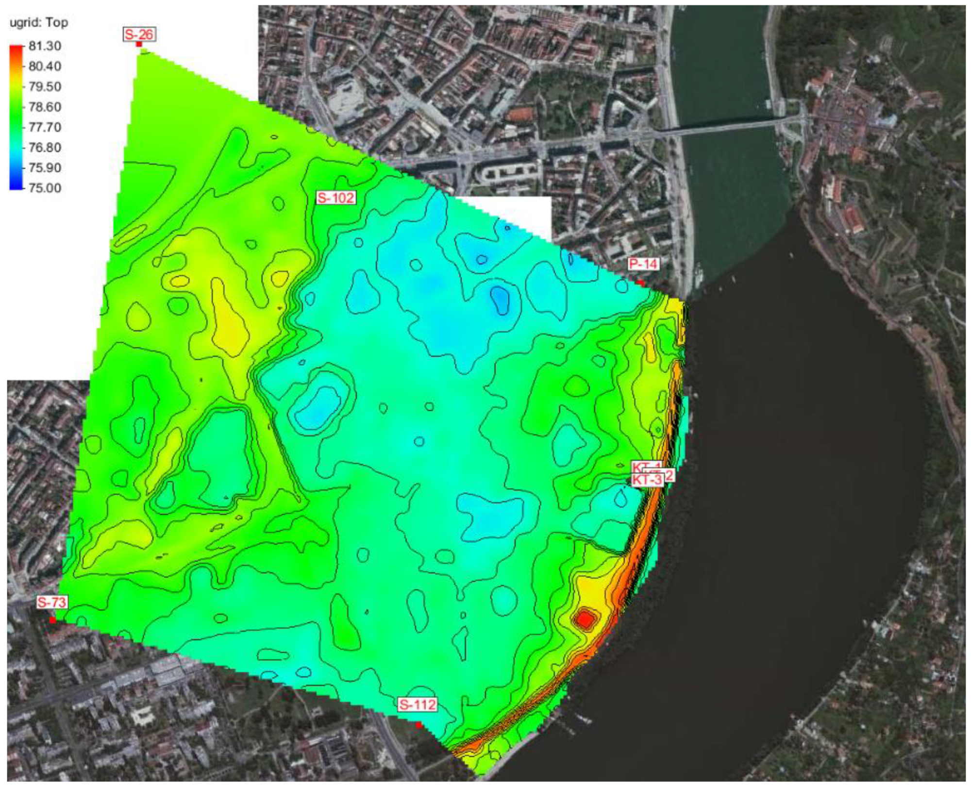
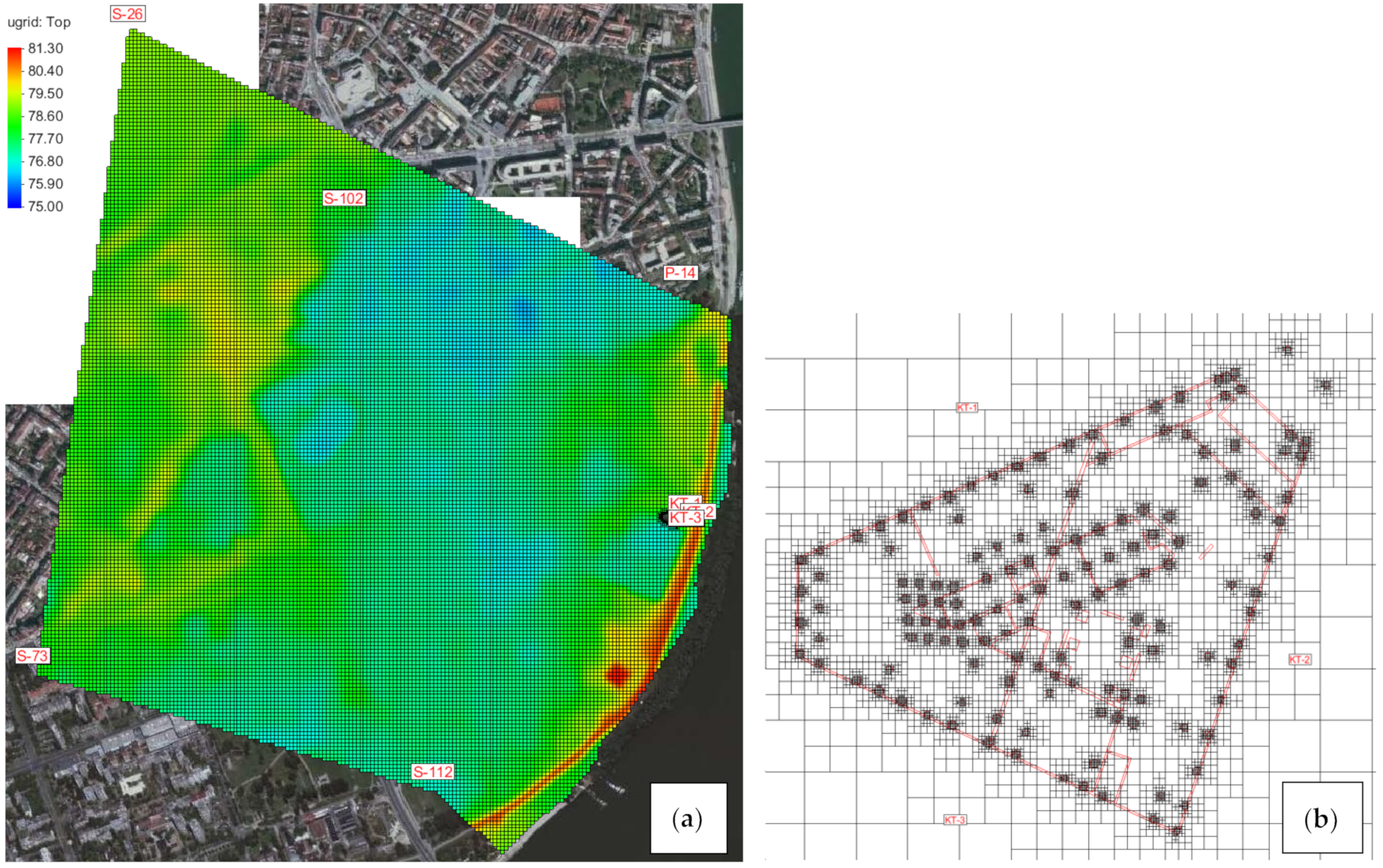
2.1. Study Area

The study area was in Novi Sad, the Republic of Serbia (Figure 1). The principal issue of the location is the proximity of the levee and, consequently, the prospective adverse impact of the structure at the location on the groundwater flow and, thus, on the stability of the levee. Since the structures in the study area are founded on piles, the piles in the soil represent a unique type of hydraulic obstacle to groundwater flow, which can result in the alteration of the flow pattern at this location positioned at a relatively short distance from the Danube River. This flow modification caused by the grid-type obstacle can produce, on the one hand, a rise in the groundwater level in the vicinity of the structure and, on the other hand, a deformation of the steady-state flow pattern at the location, caused primarily by the proximity of the Danube. The influence of the immediate vicinity of the Danube on the structure is reflected primarily in the “practically” direct connection of the waterflow and its dynamics with the site. The change in the hydraulic regime in the Danube due to its proximity is relatively quickly “transferred” to the study area, which is why this pile “structure” can significantly affect the groundwater regime both in terms of the level and flow rate in the porous medium. A sudden rise in the Danube level generally generates significant hydraulic gradients in the soil located in the close vicinity of the contact with the Danube, which inevitably leads to an increase in filtration rates. An additional reduction in the flow profile can result in an additional intensification of filtration rates at the location, which can threaten the integrity of the soil around the structure itself and its surroundings. Taking the proximity of the levee into account, it becomes clearly evident that carrying out an adequate estimation of groundwater flow at the location is necessary to determine the impact of the structure on the groundwater regime and to propose appropriate measures to eliminate negative effects. Considering the complexity of the issue in terms of the structure itself, where the foundation was made using piles of different lengths, and in terms of the proximity of the Danube and the influence of its hydraulic regime, which is primarily characterized by temporal variability, the analysis mentioned above can be conducted exclusively by applying an unsteady-state spatial mathematical model of water flow in a porous medium that can model such complex conditions.

2.2. Methodology

The Groundwater Modeling System, GMS 10.3, was chosen for the conceptual and numerical modeling. This software package incorporates the United States Geological Survey’s Modular three-dimensional Finite Differences groundwater flow code, MODFLOW-2000, the Finite Element code, FEMWATER, and several solute transport codes. Hence, there are various codes to choose from, depending on the available data and the objectives to be achieved. Both numerical groundwater flow modeling codes, MODFLOW and FEMWATER, are flexible to use in the GMS system. In this study, MODFLOW was chosen for the numerical simulation since it has been universally very well tested to simulate similar conditions in other places around the world. A basic description of the case study area was presented in the previous section. Details of the case study area in line with the GMS model framework are presented below.

2.3. Conceptual Model

The first step in building the conceptual model was defining the dimensions of the modeled area. The data used for this were those on available boreholes and levels of the Danube River. Defining the area’s dimensions primarily refers to determining the area within which the calculations will be carried out. Defining the boundaries of the model was directly determined by the sites where the available data on the measured levels were recorded, which were implemented in the model in the form of boundary conditions. In this case study, the layout plan of monitoring wells was obtained from The Urban and Spatial Planning Institute of Novi Sad, Figure 1. Given that the subject area was surrounded by wells S-73, S-112, P-14, S-102, and S-26, in which the groundwater level was continuously measured, with the Danube River on the eastern side, this area was adopted as representative for modeling purposes. The modeled area was formed by connecting boundary wells S-73, S-112, P-14, and S-26 (well S-102 was used for calibration purposes) and the Danube, thus generating a closed polygon within which a grid was formed and simulations were performed. At the well locations and the Danube, corresponding level measurements were set as boundary conditions. Interpolation was performed for each moment in time on the parts of the outline between the wells. By setting the boundary conditions in this way, an area was formed within which the flow was induced exclusively by the measured “boundary” conditions, which resulted in a more realistic picture of the groundwater hydraulic regime regarding the assumed state of the level at the boundaries.

After defining the dimensions of the model, the grid was formed. This section is significantly larger than the case study area, so the approach of using different grid resolutions was chosen for the grid formation. Namely, as the structure itself and its immediate surroundings required more attention to detail, a denser grid was used at this site—a higher resolution in the surface area of 50.0 m × 50.0 m, while a lower-resolution grid was applied for the remaining area—the grid containing the cells with dimensions 10.0 m × 10.0 m (Figure 2a). As the structure at the location is founded on piles with different diameters (0.6–0.8 m), the principle of local grid densification was used to model these elements. This procedure involved increasing the grid resolution only at the location of the case study element (i.e., the pile). In contrast, the resolution was gradually reduced in its immediate vicinity until the resolution set in the broader region was reached. The broader region contained the grid cells with dimensions 10.0 m × 10.0 m, while a higher resolution was used in the zone around the structure itself, and a cell of 0.15 m × 0.15 m was set for the section next to the piles. The obtained grid at the location of an individual pile was of such resolution that it was possible to replace one pile with several grid cells and, thus, simulate its influence on the groundwater flow at the location of the study area.

In the vertical direction, four grid layers were set to adequately cover both the impervious area’s height position and the piles’ dimensions in the vertical view. The diameter of all piles is 80 cm, while their length varies in the range of 9–13 m. The first layer extends from the surface of the terrain to an elevation of 77.46 m, the second in the range of 77.46–74.94 m, the third covers 74.94–65.94 m, and the fourth is in the region of 65.94–58.00 m. For each of these layers, corresponding values of hydraulic parameters—the filtration coefficient K and retention coefficient S—along with the parameters describing the permeability and yield of the soil were used. The geotechnical study data were used for the terrain’s vertical stratification. These data show that this location is mostly sandy land extending to the floor, estimated at an elevation of 58.0 m. It should be noted that these are data on the narrower locality around the object itself, which, due to the lack of more detailed bases, were adopted as such for the entire modeled area. The disposition of the considered layers of the analyzed area is shown in Figure 3.

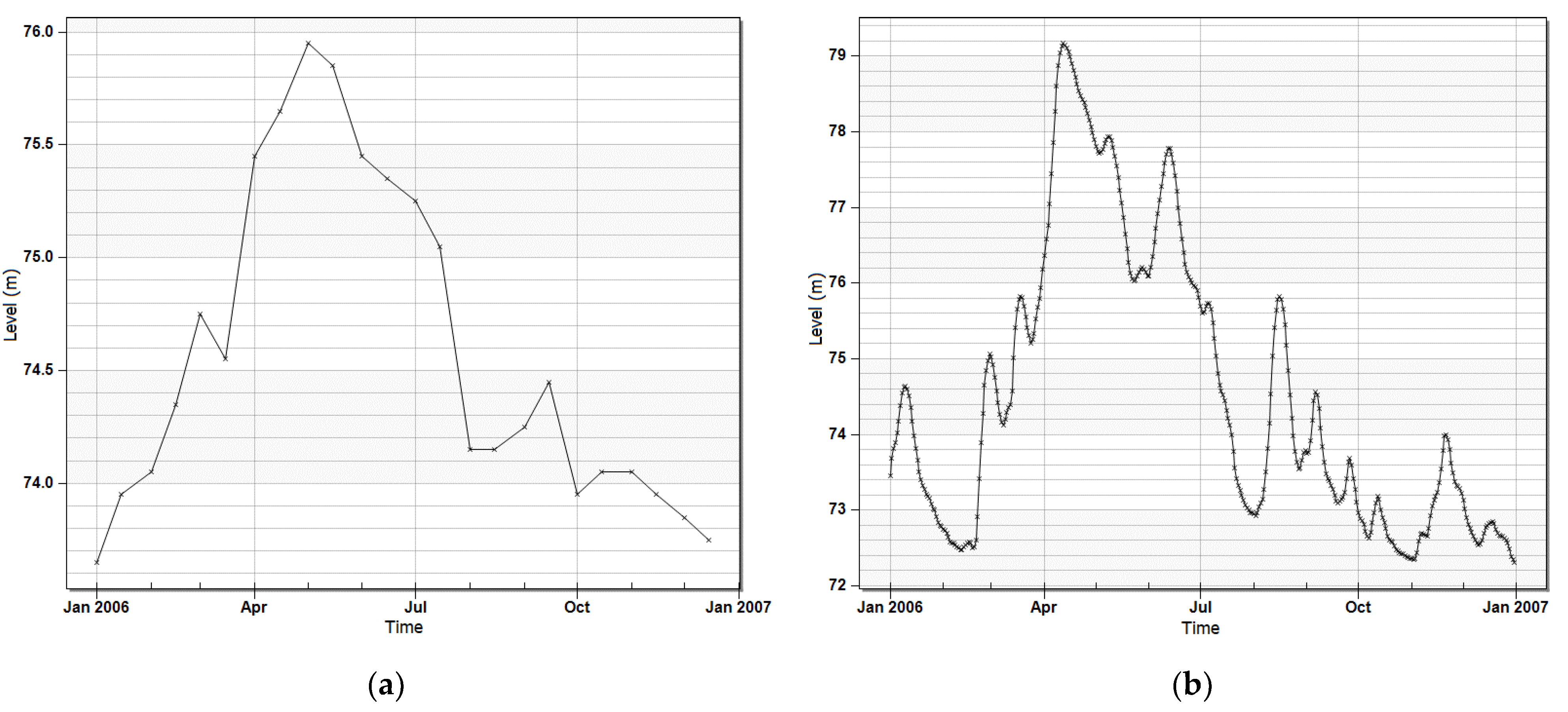
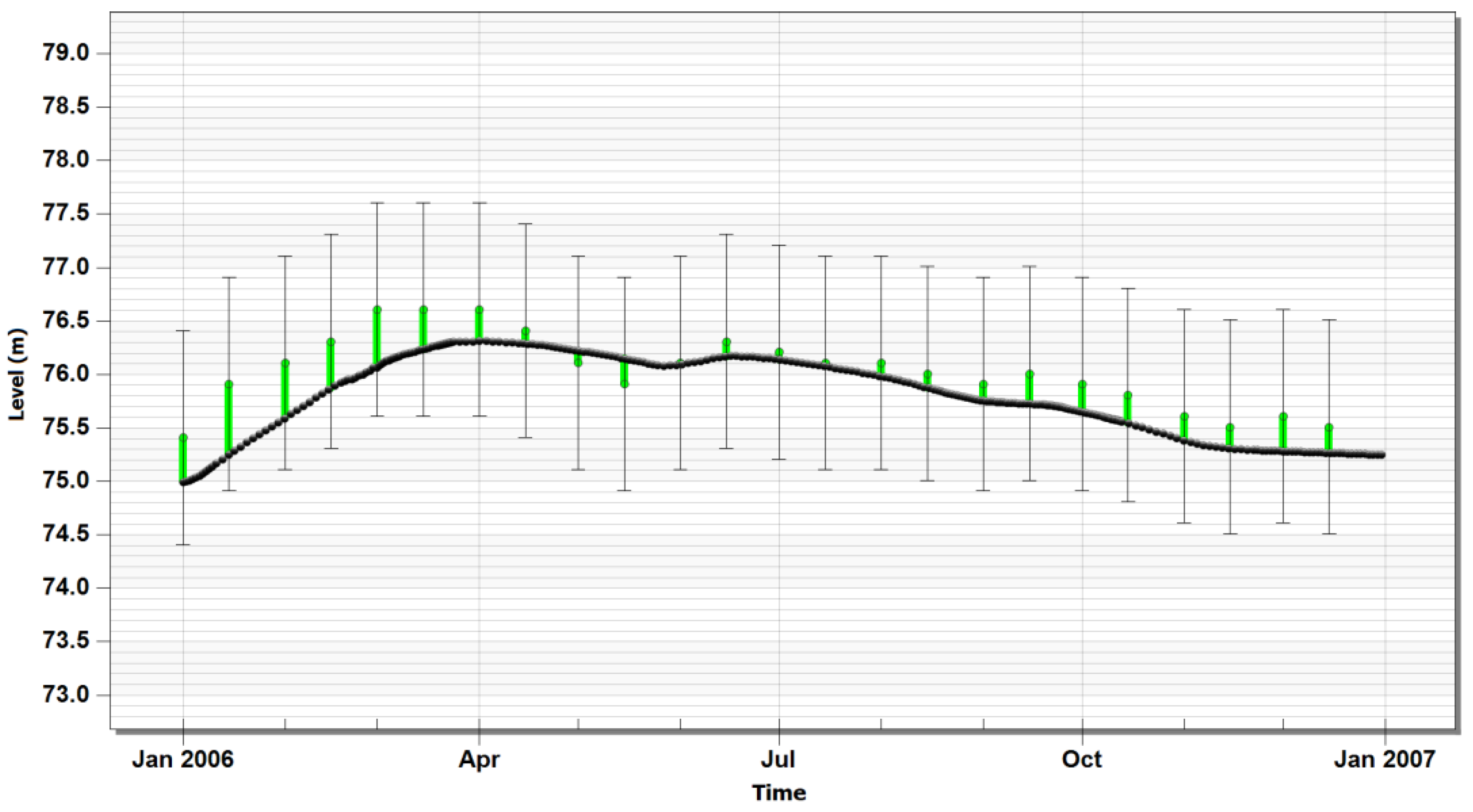
2.4. Model Calibration

The next step was to initiate the model calibration process for the previously defined model. This procedure involved varying the above-mentioned hydraulic parameters for a simulation period and comparing the obtained results with certain available measurement points within the model’s boundaries. The main goal was to obtain the best possible match between the calculated and observed values. To reproduce the groundwater regime at the given location as accurately as possible and then determine the potential impact of the structure on it, the entire year 2006 was taken as the simulation period. Transient simulation was carried out for 2006 as it was a year with extremely high water levels recorded at the hydrological station Novi Sad. For these purposes, a temporal change in the piezometric head was specified in the wells located on the boundaries of the model, and the water level graph for the year 2006 was specified on the boundary line between the modeled area and the Danube (Figure 4).

After setting boundary conditions in the form of water levels in the wells and Danube River near Novi Sad for 2006, the goal was to determine flow parameters. The calibration process was carried out by comparing the calculated water level values with the measured ones in well S-102 for different filtration coefficient values, in order to achieve the best possible match between the compared values. It should be noted that the calibration was carried out without the piles, i.e., in the calibration process the piles were not implemented in the model. For the model defined in this way, the filtration coefficient of K = 250.0 m/day and the retention coefficient of S = 0.005 1/day were determined. The comparison of the calculated and measured water levels in well S-102 for the entire simulated period of the year 2006 is presented in Figure 5. The maximum deviation is approximately 70 cm, which is acceptable regarding groundwater levels. In this period, the piles did not exist. An example of the spatial distribution of the groundwater level is shown in Figure 6, along with the detail of the structure showing three control points: KT-1, KT-2, and KT-3, located at a distance of 3.5 m from the structure itself, which can assist in comparing the temporal distribution of the groundwater levels for the year 2006 and for the two cases, i.e., with and without the structure. This allows the control of the structure’s impact on groundwater levels in its vicinity in the case of an unsteady state of the Danube regime and groundwater throughout 2006.

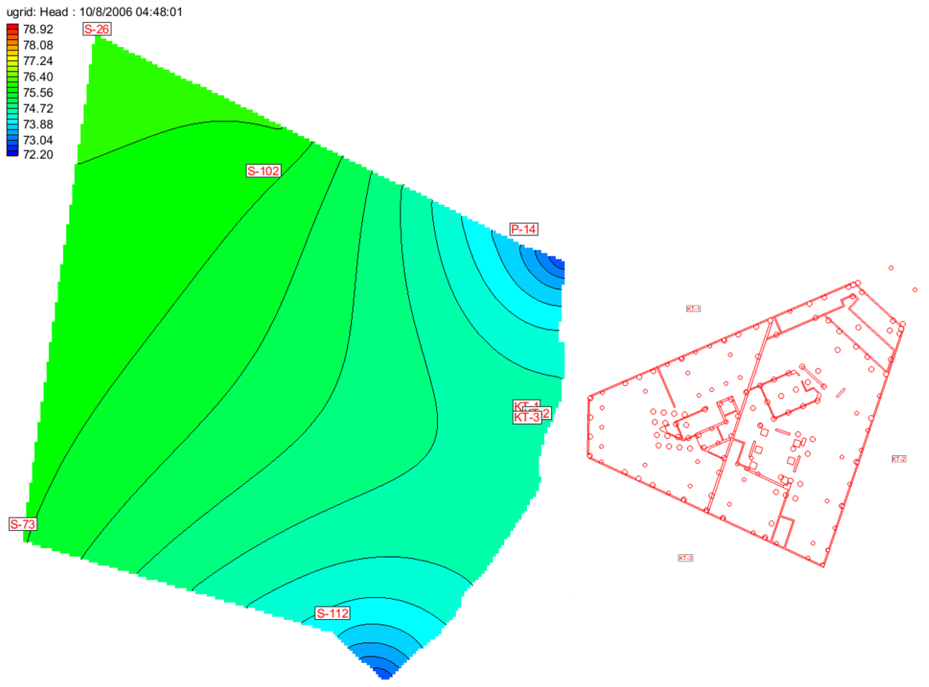
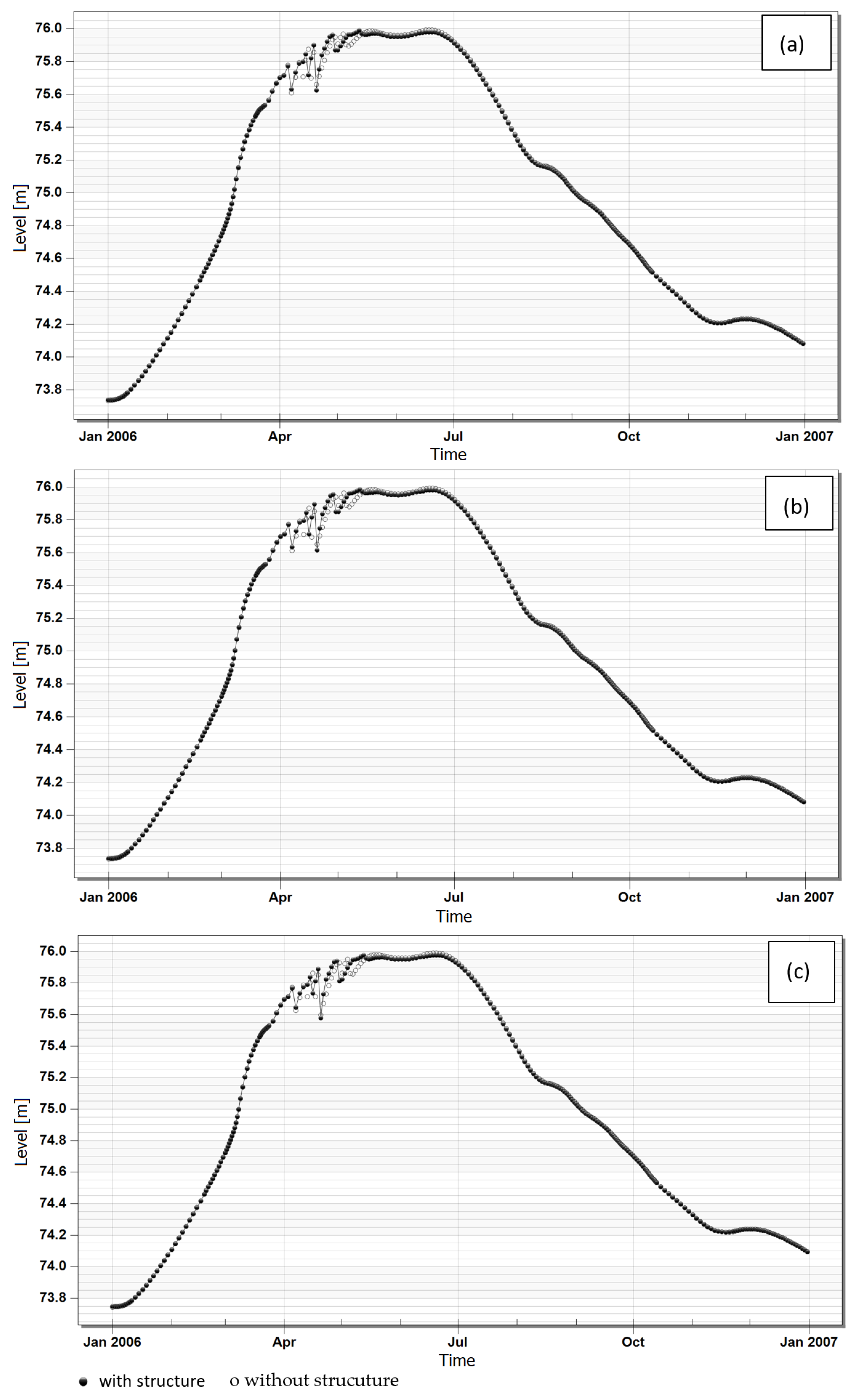
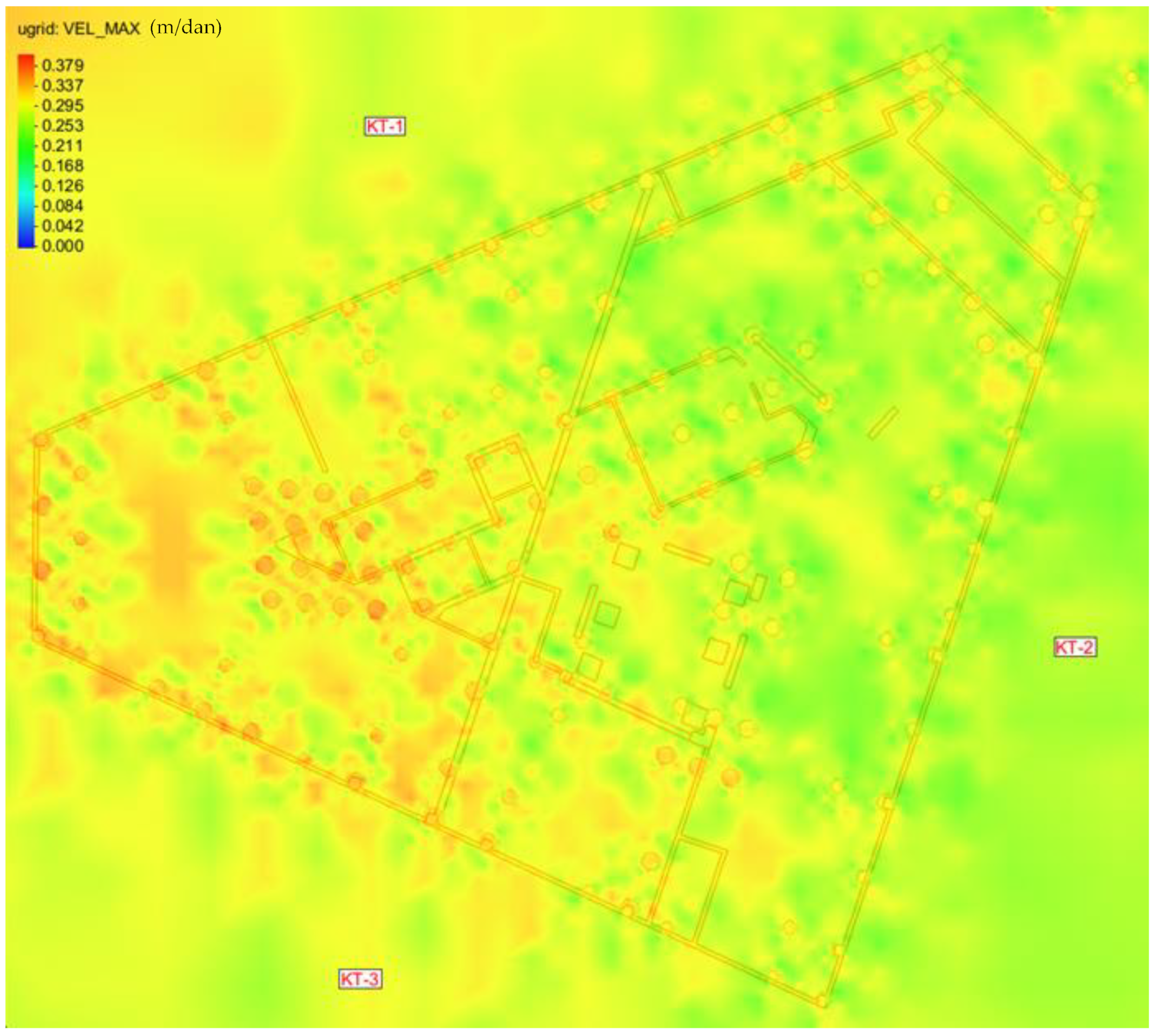
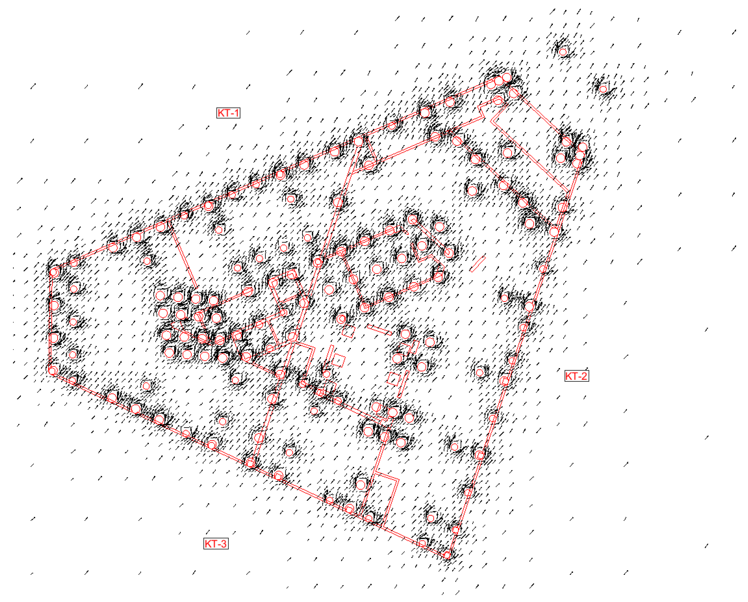
3. Results and Discussion

After the model calibration, the structure was implemented into the model according to the available layout plans. The groundwater flow in the case study location was simulated for the calibrated year 2006. Each of the piles was individually inserted into the model using the principle of “blocking” the grid cells inside the pile to the depth of 9–13 m, practically forming a no-flow zone at the position of the pile itself. For the study area location as described above, shown in Figure 2b in the form of cells in the horizontal plane, the impact of the structure on the groundwater in the surrounding area was analyzed by comparing the groundwater level change over time in three control points: KT-1, KT-2, and KT-3, in cases with and without the structure, as well as by examining the flow net at the location of the structure itself. Comparison diagrams for each control point are given in Figure 7. The maximum velocity values (in m/day) for the cases with and without the structure and an example of the resulting flow net for 9 March 2006 are shown in Figure 8, Figure 9 and Figure 10. It should be noted that the velocities presented in Figure 8 and Figure 9 are the maximum (extreme) ones. The values of these velocities are not spatially coordinated in time. In other words, they do not refer to the same moment in time at each point, but the maximum velocity recorded over the whole year is attached to each point. Numerical values of velocities in two points next to each other are mutually independent.

The obtained results indicate no influence of the piles on the groundwater flow in the study area. If the numerical oscillations of the level at the control points from April to May are excluded, the diagram lines of groundwater level change are nearly coincident for the cases with and without the structure. These oscillations are solely a consequence of the drying and wetting of cells and layers due to the temporal variation in the groundwater level. This process is numerically accompanied by minor oscillations of the level due to the permanent wetting and drying of cells. This congruence of results suggests that the structure itself does not in any way affect the groundwater levels in its immediate surroundings or in the broader region around it. On the other hand, the diagram of the maximum flow velocity values shows a slight increase in velocities in the space between the piles, i.e., along the lines of the shortest distance between two piles (Figure 9). However, the analysis of the maximum velocity values clearly demonstrates that there is only a slight (negligible) increase in the velocity in the zone between the piles. Therefore, when observing the case without the structure (Figure 8), it can be noticed that the maximum velocity values amount to around 0.35 m/day, while in the case with the structure they reach the value of 0.40 m/day (Figure 9).

4. Conclusions

This paper presents the mathematical modeling of groundwater flow in an area containing piles. Due to the complexity of the flow pattern caused by the proximity of the Danube River and the soil stratification, as well as a rather dense distribution of piles in the study area, a 3D model of water flow in a porous medium was used. The applied principles included local grid densification and the formation of no-flow zones in the piles’ positions. The impact analysis was carried out by comparing the groundwater level change over time in the immediate vicinity of the piles at three control points, along with the flow net analysis in the pile zone. The built model was first calibrated based on the available measurements, and then a simulation of the flow in the pile zone was carried out. The obtained results indicate no influence of the piles on the groundwater flow in the study area, both in terms of critical flow velocities and a possible backwater effect upstream.

A future study will be based on an improved model, within which the considered area will be expanded, and a few more years of measured data will be used in the calibration process. The goal is to complete the analysis with physical influences not considered in this paper. A numerical 3D model of groundwater flow will be created using the Lattice Boltzmann method, which, although relatively new in this field of application, has proven to be effective in groundwater modeling so far [24].

References

1. Jisun, K.; Sung-Wook, J.; Hyoun Soo, L.; Jeonghoon, L.; Ok-Sun, K.; Hyoungseok, L.; Soon Gyu, H. Hydrogeological characteristics of groundwater and surface water associated with two small lake systems on King George Island, Antarctica. J. Hydrol. 2020, 590. [Google Scholar] [CrossRef]
2. Baki, S.; Hilali, M.; Kacimi, I.; Kassou, N.; Nouayti, N.; Bahassi, A. Assessment of groundwater intrinsic vulnerability to pollution in the Pre-Saharan areas—The case of the Tafilalet plain (Southeast Morocco). Procedia Earth Planet. Sci. 2017, 17, 590–593. [Google Scholar] [CrossRef]
3. Xu, X.; Huang, G.; Qu, Z.; Pereira, L. Using MODFLOW and GIS to assess changes in groundwater dynamics in response to water saving measures in irrigation districts of the upper Yellow River basin. Water Resour. Manag. 2011, 25, 2035–2059. [Google Scholar] [CrossRef]
4. Carreira, P.M.; Bahir, M.; Ouhamdouch, S.; Fernandes, P.G.; Nunes, D. Tracing salinization processes in coastal aquifers using an isotopic and geochemical approach: Comparative studies in western Morocco and southwest Portugal. Hydrogeol. J. 2018, 26, 2595–2615. [Google Scholar] [CrossRef]
5. Moghaddam, H.K.; Moghaddam, H.K.; Kivi, Z.R.; Bahreinimotlagh, M.; Alizadeh, M.J. Developing comparative mathematic models, BN and ANN for forecasting of groundwater levels. Groundw. Sustain. Dev. 2019, 9, 100237. [Google Scholar] [CrossRef]
6. Leake, S.A.; Hoffmann, J.P.; Dickinson, J.E. Numerical ground-water change model of the C aquifer and effects of ground-water withdrawals on stream depletion in selected reaches of Clear Creek, Chevelon Creek, and the Little Colorado River, northeastern Arizona. U.S. Geol. Surv. Sci. Investig. Rep. 2005, 5277. [Google Scholar] [CrossRef]
7. Mengistu, H.; Tessema, A.; Abiye, T.; Demlie, M.; Lin, H. Numerical modeling and environmental isotope methods in integrated mine-water management: A case study from the Witwatersrand basin, South Africa. Hydrogeol. J. 2015, 23, 533–550. [Google Scholar] [CrossRef]
8. Yihdego, Y.; Danis, C.; Paffard, A. 3-D numerical groundwater flow simulation for geological discontinuities in the Unkheltseg Basin, Mongolia. Environ. Earth Sci. 2015, 73, 4119–4133. [Google Scholar] [CrossRef]
9. Yihdego, Y.; Webb, A.J.; Leahy, P. Modelling of lake level under climate change conditions: Lake Purrumbete in southeastern Australia. Environ. Earth Sci. 2015, 73, 3855–3872. [Google Scholar] [CrossRef]
10. Yidana, S.M.; Essel, S.K.; Addai, M.O.; Fynn, O.F. A preliminary analysis of the hydrogeological conditions and groundwater flow in some parts of a crystalline aquifer system: Afigya Sekyere South District, Ghana. J. Afr. Earth Sci. 2015, 104, 132–139. [Google Scholar] [CrossRef]
11. Mengistu, H.A.; Demlie, M.B.; Abiye, T.A.; Xu, Y.; Kanyerere, T. Conceptual hydrogeological and numerical groundwater flow modelling around the Moab Khutsong deep gold mine, South Africa. Groundw. Sustain. Dev. 2019, 9, 100266. [Google Scholar] [CrossRef]
12. Malekzadeh, M.; Kardar, S.; Shabanlou, S. Simulation of groundwater level using MODFLOW, extreme learning machine and Wavelet-Extreme Learning Machine models. Groundw. Sustain. Dev. 2019, 9, 100279. [Google Scholar] [CrossRef]
13. Fioreze, M.; Mancuso, A.M. MODFLOW and MODPATH for hydrodynamic simulation of porous media in horizontal subsurface flow constructed wetlands: A tool for design criteria. Ecol. Eng. 2019, 130, 45–52. [Google Scholar] [CrossRef]
14. Almuhaylan, M.R.; Ghumman, A.R.; Al-Salamah, I.S.; Ahmad, A.; Ghazaw, Y.M.; Haider, H.; Shafiquzzaman, M. Evaluating the Impacts of Pumping on Aquifer Depletion in Arid Regions Using MODFLOW, ANFIS and ANN. Water 2020, 12, 2297. [Google Scholar] [CrossRef]
15. Chakraborty, S.; Maity, K.P.; Das, S. Investigation, simulation, identification and prediction of groundwater levels in coastal areas of Purba Midnapur, India, using MODFLOW. Environ. Dev. Sustain. 2020, 22, 3805–3837. [Google Scholar] [CrossRef]
16. La Licata, I.; Colombo, L.; Francani, V.; Alberti, L. Hydrogeological Study of the Glacial—Fluvioglacial Territory of Grandate (Como, Italy) and Stochastical Modeling of Groundwater Rising. Appl. Sci. 2018, 8, 1456. [Google Scholar] [CrossRef]
17. Qiu, S.; Liang, X.; Xiao, C.; Huang, H.; Fang, Z.; Lv, F. Numerical Simulation of Groundwater Flow in a River Valley Basin in Jilin Urban Area, China. Water 2015, 7, 5768–5787. [Google Scholar] [CrossRef]
18. Aghlmand, R.; Abbasi, A. Application of MODFLOW with Boundary Conditions Analyses Based on Limited Available Observations: A Case Study of Birjand Plain in East Iran. Water 2019, 11, 1904. [Google Scholar] [CrossRef]
19. Wondzell, M.S.; LaNier, J.; Haggerty, R. Evaluation of alternative groundwater flow models for simulating hyporheic exchange in a small mountain stream. J. Hydrol. 2009, 364, 142–151. [Google Scholar] [CrossRef]
20. Li, F.; Liu, Y.; Zhao, Y.; Deng, X.; Jiang, R. Regulation of shallow groundwater based on MODFLOW. Appl. Geogr. 2019, 110, 102049. [Google Scholar] [CrossRef]
21. Phoban, H.; Seeboonruang, U.; Lueprasert, P. Numerical Modeling of Single Pile Behaviors Due to Groundwater Level Rising. Appl. Sci. 2021, 11, 5782. [Google Scholar] [CrossRef]
22. Phoban, H.; Seeboonruang, U.; Lueprasert, P. Numerical investigation on pile behavior due to the rising groundwater effect. Int. J. Geomat. 2021, 20, 171–176. [Google Scholar] [CrossRef]
23. Yuan, B.; Li, Z.; Chen, W.; Zhao, J.; Lv, J.; Song, J.; Cao, X. Influence of Groundwater Depth on Pile–Soil Mechanical Properties and Fractal Characteristics under Cyclic Loading. Fractal Fract. 2022, 6, 198. [Google Scholar] [CrossRef]
24. Budinski, L.; Fabian, J.; Stipić, M. Lattice Boltzmann method for groundwater flow in non-orthogonal structured lattices. Comput. Math. Appl. 2015, 70, 2601–2615. [Google Scholar] [CrossRef]
Figure 1. The modeled area in the broader region of the study area.
Applsci 13 13277 g001
Figure 2. The accepted grid: (a) lower resolution of the broader region; (b) higher resolution around the structure itself.
Applsci 13 13277 g002
Figure 3. The disposition of the considered layers.
Applsci 13 13277 g003
Figure 4. Adopted water level graphs for the year 2006: (a) well S-112, (b) water level of the Danube near Novi Sad.
Applsci 13 13277 g004
Figure 5. Calculated (black dots) and observed (green dots) levels in well S-102, along with the obtained deviations (green lines).
Applsci 13 13277 g005
Figure 6. Distribution of the groundwater level for 10 August 2006.
Applsci 13 13277 g006
Figure 7. Temporal distribution of groundwater level with and without structure: (a) KT-1; (b) KT-2; (c) KT-3.
Applsci 13 13277 g007
Figure 8. Maximum velocity values in case without structure.
Applsci 13 13277 g008
Figure 9. Maximum velocity values in case with structure.
Applsci 13 13277 g009
Figure 10. Flow net for 9 March 2006.
Applsci 13 13277 g010
Disclaimer/Publisher’s Note: The statements, opinions and data contained in all publications are solely those of the individual author(s) and contributor(s) and not of MDPI and/or the editor(s). MDPI and/or the editor(s) disclaim responsibility for any injury to people or property resulting from any ideas, methods, instructions or products referred to in the content.