Abstract
Smoke image segmentation plays a vital role in the accuracy of target extraction. In order to improve the performance of the traditional fire image segmentation algorithm, a new smoke segmentation method based on improved double truncation distance self-adaptive density peak clustering(TSDPC) is proposed. Firstly, the smoke image is over-segmented into multiple superpixels to reduce the time cost, and the local density of sample points corresponding to each superpixel is redefined by location information and color space information. Secondly, TSDPC combines the information entropy theory to find the optimal double truncation distance. Finally, TSDPC uses trigonometric functions to determine clustering centers in the decision diagram, which can solve the problem of over-segmentation. Then, it assigns labels to the remain sample points for obtaining the clustering result. Compared with other algorithms, the accuracy of TSDPC is increased by 5.68% on average, and the value is increased by 6.69% on average, which shows its high accuracy and effectiveness. In public dataset, TSDPC has also demonstrated its effectiveness.
1. Introduction
Image-based fire detection technology mainly includes key technologies such as fire image segmentation, feature extraction, fire judgment, and automatic fire extinguishing linkage. Fire image segmentation is the premise of fire feature extraction and recognition, and the segmentation result directly affects the accuracy of fire recognition. Therefore, the research of fire image segmentation technology is of great significance [1].
Popular fire segmentation algorithms include unsupervised fire smoke segmentation methods for infrared video [2,3], fire segmentation methods based on multi-feature fusion [4], and fire segmentation based on convolutional neural networks [5,6,7,8,9], among other methods. For example, literature [3] proposed an image-processing-based forest fire detection using infrared cameras; literature [4] proposed a mining fire warning model based on patrol robots and multi-sensor and image recognition; and literature [5] proposed a convolutional neural network (CNN)-based smoke detection and segmentation framework. These methods cover different data sources as well as different feature analysis approaches and have been widely used in smoke detection.
In the early stages of a fire outbreak, the smoke provides more timely potential information than flames [10]. Separating the target area from the background in the fire image is helpful for judging the location and hazard degree of the fire. Classical segmentation algorithms include threshold-based [11,12], region-based [13,14], and edge detection-based [15] segmentation algorithms. The threshold-based segmentation method usually only uses the pixel grayscale information of the image, does not consider the spatial correlation information between pixels, is easily affected by noise, and has poor anti-interference performance. Region-based segmentation methods tend to over-segment images. The segmentation method based on edge detection is simple and the detection speed is fast, but it is very sensitive to noise, so there will be problems such as edge blurring.
Compared with the traditional image segmentation algorithm, the high-efficiency cluster segmentation algorithm has the advantages of unsupervised learning and has achieved better results in image segmentation. Sipkens et al. [16] propose a new method for identifying soot aggregates in transmission electron microscopy images using k-means clustering. They employ background removal, denoising, and image texture measurement to preprocess the image, and then perform segmentation using rolling ball transform and K-means. However, this method has many processes and complicated technology. Zhao et al. [17] propose a novel neutrosophic image segmentation based on an improved fuzzy c-means algorithm (NIS-IFCM). They combine particle swarm optimization (PSO) and fuzzy c-means (FCM) to effectively remove image noise and make the boundaries of the segmented regions clearer. Abdullahhum et al. [18] propose CSFCM: an improved fuzzy c-means image segmentation algorithm using a collaborative approach. They use neural networks and Xie and Beni indices to determine the number of clustering centers, introduce a new meta-heuristic collaborative method to automatically determine the most suitable meta-heuristic parameters, and initialize the clustering centers. Armin Gorzary Osquie et al. [19] propose CGFFCM: clustering weights and group local feature-weight learning in a fuzzy c-means clustering algorithm for color image segmentation. They used an automatic cluster weighting scheme to reduce the sensitivity to initialization and adopted a group local feature weighting strategy to achieve better image segmentation. Yang et al. [20] propose an improved intuitionistic fuzzy c-means for ship segmentation in infrared images. They incorporate target probability information into intuitionistic FCM, using a regularized form of neighborhood information to preserve image details. This method can effectively segment infrared ship images, but it needs to manually determine the number of clusters, fuzzy factors, and other parameters. Sheng et al. [20] used a combination of SLIC and DBSCAN to achieve the segmentation of fire areas, combined with convolutional neural networks to identify fires. K-means and FCM are classic clustering algorithms, but they have many adjustment parameters and are prone to local optimal solutions. Liu et al. [21] propose an automatic segmentation of foveal avascular zone (FAZ) based on adaptive watershed algorithm in retinal optical coherence tomography angiography images. They analyze the relationship between the “dams” length and the maximum inscribed circle radius of FAZ, and propose an adaptive watershed algorithm to solve the problem of “over-segmentation”. Kang et al. [22] propose a lorenz curve-based entropy thresholding on circular histogram. They introduce the lorenz curve into circular histogram and use the entropy threshold of linearized circular histogram to select the best threshold.
Density Peak Clustering (DPC) [23] is a clustering algorithm that does not require iteration and it is widely used in image segmentation. Wang et al. [24] propose multi-center density peak clustering (McDPC). McDPC uses the assumption that the potential clustering centers are far apart to obtain representative data points and then combines the representative data points after classification. McDPC is used for image segmentation and facial recognition to obtain better experimental results. Liu et al. [25] propose a modified PageRank algorithm to compute the local density for each data point. In image segmentation, this algorithm achieves better experimental results than DPC. Zhou et al. [26] propose a linear fitting density peaks clustering algorithm for image segmentation (LDPC). They use a linear fitting method to choose clustering centers automatically; LDPC has better segmentation performance compared to DPC and K-means. Zhu et al. [27] propose medical image segmentation using fruit fly optimization and density peaks clustering. They combine DPC with the fruit fly optimization algorithm, which can automatically determine the clustering centers and truncation distance; in medical image segmentation, this algorithm has the advantages of fast convergence speed and good robustness. Guan et al. [28] propose peak-map-based fast density peak clustering for image segmentation (PGDPC). They use the KNN distance to calculate the local density and use a peak-map-based allocation strategy, which can quickly and accurately segment the image, but the number of DPC clustering centers needs to be manually selected. DPC has the advantages of fewer adjustment parameters, no need for an iterative solution, etc. However, the local density defined by the DPC algorithm does not consider the structural differences of high-dimensional data, and sometimes cannot truly reflect the local density of sample points; the truncation distance of DPC needs to be manually selected. If the truncation distance is too large or too small, the clustering effect will be worse; DPC needs to manually select the clustering center through the decision diagram. Many scholars have made improvements to the shortcomings of DPC [29,30,31,32,33].
In order to improve the segmentation accuracy of smoke images and find out the smoke regions accurately, a smoke segmentation method based on improved adaptive density peak clustering is proposed. TSDPC redefines the local density of the sample point through the density calculation equation and expands the density difference between the target area and the background. TSDPC obtains the optimal double truncation distance through information entropy theory. Then, TSDPC uses trigonometric functions to determine the number of clustering centers in the decision diagram.
2. Principle of Density Peak Clustering
The DPC algorithm is a density and distance-based clustering algorithm based on two assumptions: (1) The local density of sample points around the clustering center is low. (2) The distance between clustering centers is long [34]. After selecting the class center through the decision diagram, assign the non-clustering center samples to the category of the sample points with the larger density and the smallest distance until all the sample points are classified.
Suppose the dataset . For each data point, two parameters are calculated: local density and distance from the higher density point.
- (1)
- Calculate the local density.
The calculation method of the local density of the sample point is as follows:
where represents the Gaussian kernel function. represents the Euclidean distance from the sample point to the sample point , is a truncation distance and needs to be defined by users. Usually, the truncation distance is the value around of the neighbors [23].
- (2)
- Calculate the relative distance.
In Equation (2), is the minimum distance from data point to data point with higher local density. When the local density of data point is the largest, assign the maximum distance value to data point .
- (3)
- Select clustering centers.
Draw a decision map based on the local density and distance of data points, and manually select data points with larger density and distance as clustering centers. On the decision diagram, the point with a higher local density and larger distance can be selected as the clustering center point, and the point with small and larger can be regarded as an abnormal point. Then, the remaining data points are sequentially assigned to the cluster to which the data points with the higher local density and the closest distance belong.
3. Procedure of TSDPC
This paper proposes the TSDPC for smoke image segmentation. The overall flow of TSDPC is shown in Figure 1. The collected smoke images are used as the input of the algorithm, and the segmented smoke images are used as the output. Specific steps are as follows.
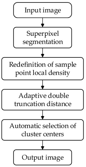
Figure 1.
Flowchart of TSDPC.
(1) Perform superpixel segmentation on the smoke image, grouping similar pixels into irregular blocks to simplify the representation of the image. The superpixel block is regarded as a sample point, and the local density of the sample point is calculated. (2) Combined with information entropy theory, TSDPC obtains the optimal double truncation distance. (3) Using the knowledge of trigonometric functions, after TSDPC automatically selects the clustering centers, the segmentation of the smoke image is completed.
3.1. Redefinition of Sample Point Local Density
In order to simplify the representation of the image, the SLIC [35] is used to aggregate similar pixels in a small area to form irregular blocks, and image blocks are used instead of pixels as a basic unit in cluster analysis. SLIC is one of the most popular superpixel generation clustering algorithms used in many image segmentation tasks [36,37]. In this paper, the initial superpixel parameter n is 500.
When traditional DPC segment images, the commonly used feature space is the CIE-Lab color space [38]. The input is the superpixel blocks of the image, which are subsequently represented by n sample points, denoted by .
When the traditional DPC algorithm divides the image, the calculated local density does not consider the structural difference of the image data, and only the color information of the image cannot truly reflect the density of the sample points. This paper redefines the density of the sample points by combining the CIE_Lab color space and position information. The local density equation of the sample points is as follows:
where represents the distance in position between the sample point and the sample point. represents the distance in CIE_Lab color space between the sample point and the sample point. and are the maximum and minimum values of , and and are the maximum and minimum values of. Normalize and to obtain and . Where indicates that the position information and CIE_Lab space distances together determine the density of sample points. As shown in Figure 2, C is the sample point to be calculated, the blue sample point E is its nearest neighbor, and the white sample point D is a non-neighbor and is its truncated distance. we suppose that the color and brightness information between adjacent sample points are quite different. In that case, even if the location difference between sample points is small, this point is not considered when calculating the local density.
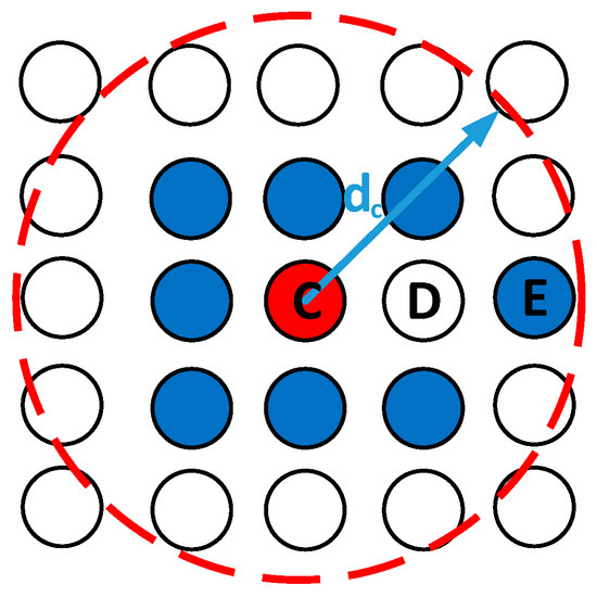
Figure 2.
Schematic diagram of sample point C density calculation.
In DPC [21], the density of sample point C is mainly determined by all sample points within the truncation distance . However, in Figure 2, the density of sample point C is mainly determined by the blue sample points within the truncation distance . Although sample point D is adjacent to sample point C, in the CIE_Lab space, the distance between the two is relatively large; thus, sample point D cannot determine the density of point C. Although sample point E is not adjacent to sample point C, its position and color space are within the truncation distance, so sample point E and other blue sample points jointly determine the density of sample point C.
3.2. Adaptation of Double Truncation Distance
Manual selection of truncation distance based on experience is one of the disadvantages of DPC. The local density redefinition in this paper is jointly determined by the location information and the CIE_Lab color space; thus, this paper will use the Hungarian mathematician Renyi in 1961 to propose an information entropy [39] that can measure the continuous random variable, and solve the optimal double truncation distance.
In information theory, information entropy is a systematic and orderly measurement method. The calculation equation of information entropy is as follows:
, in Equation (5), is the probability of the event I, and .
Before determining the density of sample points according to Equation (4), the truncation distance needs to be determined by information entropy.
TSDPC uses the information entropy theory to judge the clustering effect of the sample points. If the information entropy of the sample set is large, it means that the clustering effect of the sample set is poor; otherwise, it means that the clustering effect of the sample set is better. The information entropy of the sample set can be expressed as:
We respectively normalize the distances of all sample points in the CIE_Lab space and sort them in ascending order. Through Equations (4) and (6), the truncation distance gradually increases from to , and the interval is , find the value of the minimum entropy corresponding to the abscissa, and use this value as the truncation distance of the sample point in the position and CIE_Lab space, respectively. The specific steps of the algorithm are shown in Algorithm 1.
| Algorithm 1: Adaptation of double truncation distance |
| 1: Input: 2: For to , interval is , do |
| 3: Calculate the information entropy function and display the result in an entropy diagram; |
| 4: end for |
| 5: Find the double truncation distance corresponding to the minimum entropy value; 6: Output: |
The more similar the brightness and color of two superpixels in an image, the more similar the density between them. In this case, it is easier for two superpixels to be clustered into the same class. The location information and density of two superpixels in the image are similar, but the color and brightness information are quite different; thus, the two superpixels cannot be clustered into one class. We adopt Equation (7) to calculate the distance of the input sample points.
where and are the local density of the and sample points calculated by Equation (4). is calculated by Equation (3). Only when the local density of the sample point is the maximum density, the distance takes the maximum value of the distance of each sample point. If is not the maximum density, then the distance is the sample point distance that is denser than it and has the smallest relative distance.
3.3. Automatic Selection of Clustering Centers
One of the disadvantages of the DPC algorithm is that it requires the manual selection of clustering centers. Before selecting the clustering center, it is necessary to calculate the decision value γ of each sample point, and then artificially select the sample point with a large value as the clustering center. The decision value is calculated by Equation (8).
Usually, the decision value of the clustering center is much larger than the decision value of other sample points. According to this feature, this paper uses the sample point with the largest slope difference between the two straight lines as the number of clustering centers.
The decision values are normalized and processed in descending order. Figure 3 is a schematic diagram of the decision diagram, represents the total number of sample points, and represents the decision value of the sample point, in which there are sample points; the decision value of sample point is , and the decision value of sample point is . The number of clustering centers is usually greater than one but less than the total number of sample points. We take these two points as fixed points and connect the intermediate sample points to obtain two straight lines. Then, we calculate the tangent value.
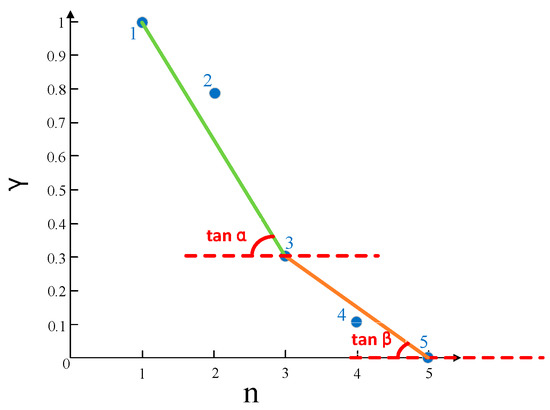
Figure 3.
Automatic selection of clustering centers via tangent value calculation.
We calculate the absolute value of the tangent of the angle between the two straight lines and the horizontal line. In order to avoid the problem of too many clustering centers, it needs to be restricted, which is expressed as:
where is the total number of sample points, is the number of sample points, and the number of sample points corresponding to the maximum value of is that of clustering centers. Algorithm 2 shows the adaptive selection of clustering centers. We normalize the decision values and process them in descending order, obtain a descending sequence , presenting the decision values in a decision diagram with two auxiliary lines for each sample point in 2nd to st, respectively. Calculate the tangent value of the sample points and substitute it into Equation (9), then we obtain the sequence . Find the number of sample points corresponding to the largest value of in the sequence; is the number of adaptively selected clustering centers.
| Algorithm 2: Automatic selection of clustering centers |
| 1: Input: Decision value ; 2: Normalization: get a descending sequence ; 3: Do the auxiliary line to get the tangent value; |
| 4: For to , do |
| 5: Calculate the value and get the sequence ; |
| 6: end for 7: Find the sequence number corresponding to the maximum value in the sequence ; 8: Output: cluster center |
4. Results
4.1. Experimental Design
The accuracy rate (), precision rate (), recall rate (), and F-measure () are used as the evaluation indicators.
where the represents the number of pixels that are correctly segmented into the smoke area; the is the number of pixels incorrectly segmented into the smoke area; the is the number of pixels incorrectly segmented into the background area; the is the number of pixels that are correctly segmented into the background.
In order to better verify the accuracy of TSDPC for fire smoke image segmentation, this paper also uses the mean intersection over union (mIoU) and volume overlap error (VOE) to evaluate the performance of the model. The larger the mIoU or the smaller the VOE, the better the segmentation effect. The mIoU is calculated by Equation (14).
where, since each pixel in the image has a category label, we assume that the total number of categories is , including object categories and background. represents the number of pixels of category predicted to be category .
The VOE is calculated by Equation (15).
where indicates the predicted smoke area; indicates the real smoke area.
4.2. Results and Analysis
4.2.1. Parameter Analysis
The proposed TSDPC only needs one essential superpixel parameter, namely the initial number of superpixels. The results under the different number of superpixels are shown in Figure 4.
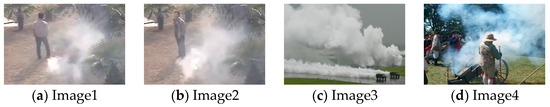
Figure 4.
Smoke images for parameter analysis.
TSDPC can segment the smoke image to some extent by selecting different initial superpixels. Figure 4 are the smoke segmentation images for parameter analysis. As shown in Figure 5a,b, TSDPC do not perform well, due to the small superpixel parameter; the superpixel parameter is large, and the segmentation effect of TSDPC has little change. For image1 and image3, the effect increases first and then tends to stabilize. For image2, the effect fluctuates greatly, and it is best when the superpixel parameter is 500. For image4, the variation of and are smooth. Therefore, we suggest that the initial superpixel parameter set in this paper is 500.
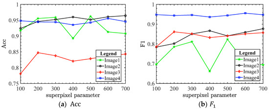
Figure 5.
Relationship between the evaluation criteria (,) and superpixel parameter on TSDPC.
4.2.2. Self-Built Dataset
We collect smoke images to evaluate them both subjectively and objectively, and six representative images are used to demonstrate the results of different methods in Figure 6. The objective evaluation is based on the manually marked smoke area.
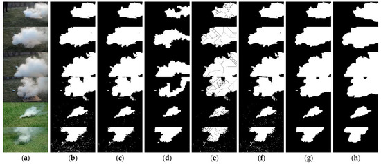
Figure 6.
Segmentation results of different algorithms. (a) Original image; (b) FCM; (c) K- means; (d) DPC; (e) Watershed; (f) MIT; (g) TSDPC; (h) Manually labeled image.
A subjective evaluation can be observed from Figure 6 that TSDPC separates the smoke area from the background, which is more complete than the areas extracted by other algorithms. To verify the segmentation effect of TSDPC in smoke images, the TSDPC is compared with FCM, K-means, DPC, Watershed, and Mean Iteration Threshold (MIT), respectively. Both the TSDPC and the five comparison algorithms can segment the smoke area. In the first four smoke images in Figure 6, the DPC algorithm (Figure 6d) cannot completely segment the smoke region, and the edges of the segmented regions by other algorithms are not smooth enough compared with TSDPC (Figure 6g). In the last two smoke images in Figure 6, the segmentation results of the TSDPC and the DPC algorithm are better and closer. While other algorithms can segment most areas of smoke, they are severely affected by noise. In the 22 smoke images, the evaluation indicators data of five clustering algorithms such as TSDPC are shown in Table 1.

Table 1.
Evaluation indicators of data statistics of six clustering algorithms (In %).
The and indicators are sometimes contradictory, so the indicator is needed to evaluate image segmentation accuracy. The results in Table 1 show that the TSDPC outperforms other segmentation algorithms proposed in this paper. Experimental data show that TSDPC has better segmentation quality. Compared with FCM, K-means, DPC, Watershed, and MIT, the accuracy of TSDPC is increased by 5.78%, 3.59%, 6.46%, 6.60%, and 5.95%, respectively; the value is increased by 6.02%, 3.67%, 9.32%, 7.72%, 6.70%, respectively.
4.2.3. Public Dataset
- (1)
- There are 143 smoke images and ground truth maps in the public dataset-1 (https://github.com/rekon/Smoke-semantic-segmentation accessed on 29 December 2022). To verify the segmentation effect of TSDPC in smoke images, the TSDPC is compared with PGDPC [28], PSO [40], respectively. The average results of each algorithm in the public dataset are shown in the following Table 2.
Table 2. Evaluation indicators data statistics of three clustering algorithms on the public dataset-1.
From Table 2, it is obvious that TSDPC is 19.17% and 12.13% higher than PGDPC in and , respectively. The difference between TSDPC and PSO on is small, but TSDPC is 5.46% higher than PSO in .
- (2)
- There are 400 smoke images and ground truth maps in the public dataset-2 (https://github.com/sonvbhp199/Unet-Smoke, accessed on 31 December 2022). The smoke images in this dataset have a more complex background environment than the previous smoke images. To further validate the segmentation effect of TSDPC in smoke images, TSDPC is compared with PGDPC [28] and PSO [40], respectively. The average results of each algorithm in the public dataset are shown in the following Table 3.
Table 3. Evaluation indicators data statistics of three clustering algorithms on the public dataset-2.
From Table 3, TSDPC has the smallest VOE, and it is obvious that TSDPC is 12.86%, 4.43%, and 10.02% higher than PGDPC in , , and mIoU, respectively. TSDPC is 5.7%, 4.61%, and 4.28% higher than PSO in , , and mIoU, respectively. In more complex public datasets, TSDPC achieves the best results compared to the other two methods.
4.2.4. Ablation Experiment
To fully illustrate the effect of the superpixel module in TSDPC on the segmentation effect of smoke images, ablation experiments are designed to verify the effectiveness of the superpixel module. Figure 7a shows the smoke images with pixel.
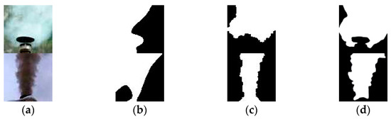
Figure 7.
Segmentation results with and without superpixel module. (a) Smoke image; (b) no super -pixel module; (c) with superpixel module; (d) manually labeled image.
Figure 7 shows that TSDPC with the superpixel module (Figure 7c) has more accurate segmentation results than Figure 7b. The and metrics of TSDPC are higher than those of TSDPC without the superpixel module. The computation time of TSDPC without the super pixel module is 2715 times longer than that of TSDPC with the super pixel module to obtain segmentation results within an acceptable time frame. Therefore, the super pixel module is valid for TSDPC.
4.3. Discussion
Usually, TSDPC divides the smoke image into two categories: foreground and background, but there are also cases where TSDPC divides the smoke image into three categories. As shown in Figure 8, the selection of the number of clustering centers affects the segmentation results. Figure 8b is the clustering result of TSDPC, which divides the smoke image into three categories. Figure 8c is the manual selection of two clustering centers, and the result does not separate the smoke area.
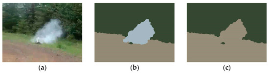
Figure 8.
TSDPC output image. (a) original smoke image; (b) TSDPC result map (the number of clustering centers is 3); (c) manually determine 2 clustering centers area.
5. Conclusions
This paper proposes a novel smoke image segmentation method, named TSDPC. TSDPC redefines the local density of sample points by using position information and CIE_Lab spatial information, and obtains an adaptive double truncation distance based on the information entropy theory. After using the knowledge of trigonometric functions in mathematics to automatically select the clustering centers, the allocation of the remaining sample points is completed. Compared with DPC, the and value of TSDPC are improved by 6.46% and 9.32%, indicating that TSDPC can overcome the problems of over-segmentation and low segmentation accuracy of smoke images. In the future, we will incorporate the unique information of smoke to improve the segmentation accuracy under complex scenes, such as small smoke areas.
Author Contributions
Conceptualization, Z.M. and L.S.; methodology, L.S.; software, Y.C.; validation, J.Z.; formal analysis, J.Z.; investigation, Y.C.; resources, Z.M.; data curation, F.H.; writing—original draft preparation, Y.C.; writing—review and editing, F.H. and L.S.; visualization, F.H.; supervision, Z.M. and L.S.; project administration, L.S.; funding acquisition, Z.M. All authors have read and agreed to the published version of the manuscript.
Funding
This research was funded by the Key Research and Development Project of Shaanxi Province (No.2020GY-186), and it was also funded by the National Natural Science Foundation of China (No.62276207).
Data Availability Statement
Data is unavailable due to privacy restrictions.
Conflicts of Interest
The authors declare no conflict of interest.
References
- Ibragimov, A.; Pleteit, H.; Pille, C.; Lang, W. A Thermoelectric Energy Harvester Directly Embedded Into Casted Aluminum. Electron Device Lett. IEEE 2012, 33, 233–235. [Google Scholar] [CrossRef]
- Ajith, M.; Martínez-Ramón, M. Unsupervised Segmentation of Fire and Smoke from Infra-Red Videos. IEEE Access 2019, 7, 182381–182394. [Google Scholar] [CrossRef]
- Ya’Acob, N.; Najib, M.; Tajudin, N.; Kassim, M. Image Processing Based Forest Fire Detection using Infrared Camera. J. Phys. Conf. Ser. 2021, 1768, 012014. [Google Scholar] [CrossRef]
- Miao, K.; Ma, J.; Li, Z.; Zhao, Y.; Zhu, W. Research on multi feature fusion perception technology of mine fire based on inspection robot. J. Phys. Conf. Ser. 2021, 1955, 012064. [Google Scholar] [CrossRef]
- Khan, S.; Muhammad, K.; Hussain, T.; Del Ser, J.; Cuzzolin, F.; Bhattacharyya, S.; de Albuquerque, V.H.C. DeepSmoke: Deep Learning Model for Smoke Detection and Segmentation in Outdoor Environments. Expert Syst. Appl. 2021, 182, 115125. [Google Scholar] [CrossRef]
- Wang, Z.; Zheng, C.; Yin, J.; Tian, Y.; Cui, W. A Semantic Segmentation Method for Early Forest Fire Smoke Based on Concentration Weighting. Electronics 2021, 10, 2675. [Google Scholar] [CrossRef]
- Wen, J.L.; Burke, M. Wildfire Smoke Plume Segmentation Using Geostationary Satellite Imagery. arXiv 2021, arXiv:2109.01637. preprint. [Google Scholar]
- Cui, W. Semantic Segmentation and Analysis on Sensitive Parameters of Forest Fire Smoke Using Smoke-Unet and Landsat-8 Imagery. Remote Sens. 2021, 14, 45. [Google Scholar]
- Vieira, P. Real-Time Integration of Segmentation Techniques for Reduction of False Positive Rates in Fire Plume Detection Systems during Forest Fires. Remote Sens. 2022, 14, 2701. [Google Scholar]
- Sheng, D.; Deng, J.; Xiang, J. Automatic Smoke Detection Based on SLIC-DBSCAN Enhanced Convolutional Neural Network. IEEE Access 2021, 9, 63933–63942. [Google Scholar] [CrossRef]
- Gritzman, A.D.; Aharonson, V.; Rubin, D.M.; Pantanowitz, A. Automatic computation of histogram threshold for lip segmentation using feedback of shape information. Signal Image Video Process. 2016, 10, 869–876. [Google Scholar] [CrossRef]
- Siri, S.K.; Kumar, S.P.; Latte, M.V. Threshold-Based New Segmentation Model to Separate the Liver from CT Scan Images. IETE J. Res. 2020, 4, 4468–4475. [Google Scholar] [CrossRef]
- Cheng, Z.; Wang, J. Improved region growing method for image segmentation of three-phase materials. Powder Technol. 2020, 368, 80–89. [Google Scholar] [CrossRef]
- Borges, V.R.; de Oliveira, M.C.F.; Silva, T.G.; Vieira, A.A.H.; Hamann, B. Region Growing for Segmenting Green Microalgae Images. IEEE/ACM Trans. Comput. Biol. Bioinform. 2018, 15, 257–270. [Google Scholar] [CrossRef] [PubMed]
- Shang, R.; Lin, J.; Jiao, L.; Yang, X.; Li, Y. Superpixel Boundary-based Edge Description Algorithm for SAR Image Segmentation. IEEE J. Sel. Top. Appl. Earth Obs. Remote Sens. 2020, 13, 1972–1985. [Google Scholar] [CrossRef]
- Sipkens, T.A.; Rogak, S. Technical note: Using k-means to identify soot aggregates in transmission electron microscopy images. J. Aerosol Sci. 2021, 152, 105699. [Google Scholar] [CrossRef]
- Zhao, J.; Wang, X.; Li, M. A Novel Neutrosophic Image Segmentation Based on Improved Fuzzy C-Means Algorithm (NIS-IFCM). World Sci. Publ. Co. 2020, 34, 2055011. [Google Scholar] [CrossRef]
- Abdellahoum, H.; Mokhtari, N.; Brahimi, A.; Boukra, A. CSFCM: An improved fuzzy C-Means image segmentation algorithm using a cooperative approach. Expert Syst. Appl. 2021, 166, 114063. [Google Scholar] [CrossRef]
- Oskouei, A.G.; Hashemzadeh, M.; Asheghi, B.; Balafar, M.A. CGFFCM: Cluster-weight and Group-local Feature-weight learning in Fuzzy C-Means clustering algorithm for color image segmentationt. Appl. Soft Comput. 2021, 113, 108005. [Google Scholar] [CrossRef]
- Yang, F.; Liu, Z.; Bai, X.; Zhang, Y. An Improved Intuitionistic Fuzzy C-Means for Ship Segmentation in Infrared images. IEEE Trans. Fuzzy Syst. 2020, 30, 332–344. [Google Scholar] [CrossRef]
- Liu, J.; Yan, S.; Lu, N.; Yang, D.; Fan, C.; Lv, H.; Yu, Y. Automatic segmentation of foveal avascular zone based on adaptive watershed algorithm in retinal optical coherence tomography angiography images. J. Innov. Opt. Health Sci. 2022, 15, 2242001. [Google Scholar] [CrossRef]
- Kang, C.; Wu, C.; Fan, J. Lorenz Curve-Based Entropy Thresholding on Circular Histogram. IEEE Access 2020, 8, 17025–17038. [Google Scholar] [CrossRef]
- Rodriguez, A.; Laio, A. Clustering by fast search and find of density peaks. Science 2014, 344, 1492–1496. [Google Scholar] [CrossRef]
- Wang, Y.; Wang, D.; Zhang, X.; Pang, W.; Miao, C.; Tan, A.H.; Zhou, Y. McDPC: Multi-center density peak clustering. Neural Comput. Appl. 2020, 32, 13465–13478. [Google Scholar] [CrossRef]
- Liu, Q.; Zhang, R.; Liu, X.; Liu, Y.; Zhao, Z.; Hu, R. A novel clustering algorithm based on PageRank and minimax similarity. Neural Comput. Appl. 2019, 31, 7769–7780. [Google Scholar] [CrossRef]
- Zhou, Y.; Zhao, T.; Wang, Y.; Wu, J.; Zhou, X. A Linear Fitting Density Peaks Clustering Algorithm for Image Segmentation. Tehnicki Vjesnik 2018, 25, 808–812. [Google Scholar]
- Zhu, H.; He, H.; Xu, J.; Fang, Q.; Wang, W. Medical Image Segmentation Using Fruit Fly Optimization and Density Peaks Clustering. Comput. Math. Methods Med. 2018, 2018, 3052852. [Google Scholar] [CrossRef]
- Guan, J.; Li, S.; He, X.; Chen, J. Peak-graph-based fast density peak clustering for image segmentation. IEEE Signal Process. Lett. 2021, 28, 897–901. [Google Scholar] [CrossRef]
- Du, M.; Ding, S.; Xu, X.; Xue, Y. Density peaks clustering using geodesic distances. Int. J. Mach. Learn. Cybern. 2018, 9, 1335–1349. [Google Scholar] [CrossRef]
- Lv, Y.; Liu, M.; Xiang, Y. Fast Searching Density Peak Clustering Algorithm Based on Shared Nearest Neighbor and Adaptive Clustering Center. Symmetry 2020, 12, 2014. [Google Scholar] [CrossRef]
- Wang, S.; Li, Q.; Zhao, C.; Zhu, X.; Yuan, H.; Dai, T. Extreme Clustering—A Clustering Method via Density Extreme Points. Inf. Sci. 2021, 542, 24–39. [Google Scholar] [CrossRef]
- Sun, L.; Qin, X.; Ding, W.; Xu, J.; Zhang, S. Density peaks clustering based on k-nearest neighbors and self-recommendation. Int. J. Mach. Learn. Cybern. 2021, 12, 1913–1938. [Google Scholar] [CrossRef]
- Cai, J.; Wei, H.; Yang, H.; Zhao, X. A Novel Clustering Algorithm based on DPC & PSO. IEEE Access 2020, 8, 188200–188214. [Google Scholar]
- Bie, R.; Mehmood, R.; Ruan, S.; Sun, Y.; Dawood, H. Adaptive fuzzy clustering by fast search and find of density peaks. Pers. Ubiquitous Comput. 2016, 20, 785–793. [Google Scholar] [CrossRef]
- Achanta, R.; Shaji, A.; Smith, K.; Lucchi, A.; Fua, P.; Süsstrunk, S. SLIC Superpixels Compared to State-of-the-Art Superpixel Methods. IEEE Trans. Pattern Anal. Mach. Intell. 2012, 34, 2274–2282. [Google Scholar] [CrossRef] [PubMed]
- Han, C. Improved SLIC imagine segmentation algorithm based on K-means. Clust. Comput. 2017, 20, 1017–1023. [Google Scholar] [CrossRef]
- Di, S.; Liao, M.; Zhao, Y.; Li, Y.; Zeng, Y. Image superpixel segmentation based on hierarchical multi-level LI-SLIC. Opt. Laser Technol. 2021, 135, 106703. [Google Scholar] [CrossRef]
- Sharma, G.; Wu, W.; Dalal, E.N. The CIEDE2000 color-difference equation: Implementation notes, supplementary test data, and mathematical observations. Color Res. Appl. 2005, 30, 21–30. [Google Scholar] [CrossRef]
- Renyi, A. On measures of entropy and information. In Proceedings of the 4th Berkeley Symposium on Mathematics, Statistics and Probability, Berkeley, CA, USA, 20 June–30 July 1960. [Google Scholar]
- Mousavi, S.M.H.; Victorovich, L.; Ilanloo, A.; Mirinezhad, S.Y. Fatty Liver Level Recognition Using Particle Swarm optimization (PSO) Image Segmentation and Analysis. In Proceedings of the 2022 12th International Conference on Computer and Knowledge Engineering (ICCKE), Virtual, 17–18 November 2022; pp. 237–245. [Google Scholar]


Disclaimer/Publisher’s Note: The statements, opinions and data contained in all publications are solely those of the individual author(s) and contributor(s) and not of MDPI and/or the editor(s). MDPI and/or the editor(s) disclaim responsibility for any injury to people or property resulting from any ideas, methods, instructions or products referred to in the content. |
© 2023 by the authors. Licensee MDPI, Basel, Switzerland. This article is an open access article distributed under the terms and conditions of the Creative Commons Attribution (CC BY) license (https://creativecommons.org/licenses/by/4.0/).