Study on the Degradation Law of Artificial Joint Surfaces with Natural Morphologies under Quasi-Static Cyclic Shearing

Abstract

In this paper, a series of quasi-static cyclic shear tests were performed on artificial rock joint specimens with natural morphologies at different normal stress levels. After shearing, combined with 3D scanning technology and image processing, the 3D morphology parameter, $A_0{\theta }_{max}^{\ast }/\left(C+1\right)$, of 36 analyzed directions was measured to investigate the damage and degradation laws of the joint surfaces. The polar curves of the roughness parameter shrank from a circular to an elliptical shape, with the shear direction as the minor axis. The roughness degradation rates and the shear cycles were mutually interrelated with the normal stress levels, which had a tendency to be fast initially and then to slow down under higher normal stress. Influenced by the cyclic shear direction, the 3D roughness of the joint surfaces degenerated anisotropically and sustained the most serious damage along the shear direction. Two damage and degradation fitting formulas were proposed, which could aid the assessment of residual roughness under different stress histories and the cumulative wear degree.

1. Introduction

The joints in engineering rock mass may undergo reciprocating shear dislocation under seismic or blasting loads, resulting in their wear and degradation and in the weakening of their mechanical properties. Therefore, the study of the damage accumulation and degradation mechanism of rock joints under reciprocating loads is significant.

Over the past few decades, the cyclic loading protocol has been considered an effective method for studying the mechanical behavior of rock joints under dynamic loading. In terms of the research on the mechanical properties of joints under cyclic loading, the representative studies are those conducted by Jing [1], Huang [2], Fox [3,4], Homand [5], Lee [6], and Jafari [7]. Other similar studies [8,9,10,11,12,13] have shown that the mechanical behavior of joints is related to the number of load cycles, joint asperity, and loading boundary conditions.

The roughness and the shear strength of the joint plane have a stable relationship, so a quantitative relationship can be established between them. At present, the two-dimensional profile line methods used to describe rock surface morphology can be divided into the description of the morphology line height difference parameter, the description of the morphology line texture parameter, the description of the fractal effects, and the description of the JRC curve. The height difference parameter description of the morphology line is a parameter used to describe the variation in the morphology height distribution [14], including the average height of the center line Z₀, the height root mean square Z₁, and other indexes. The texture parameter description of the morphology lines is used to study the convex shape and other information about the surface [15], including the root mean square Z₂ of the first derivative of the surface morphology and the root mean square Z₃ of the second derivative of the surface morphology. Barton [16] conducted direct shear tests on 136 joint plane samples and grouped them to obtain 10 standard JRC curves. The three-dimensional roughness parameter can describe the surface morphologies of joints more accurately and reasonably. Belem et al. [5,17] proposed five morphological parameters to describe the three-dimensional joint surface roughness, including the mean shear inclination angle of the joint surface ${\theta }_s$, surface roughness coefficient R_s, anisotropy coefficient K_a, joint surface bending degree T_s, and morphology roughness degree ${\theta }_{p+}$, ${\theta }_{p-}$. Grasselli [18,19] found that only the joint elements with positive slope angles in the shear direction contributed to the shear strength. Grasselli [18,19] also found, for the first time, that the rock joints’ three-dimensional morphologic parameters were related to the shear strength, and the parameters $A_0$ (the maximum possible contact area) and ${\theta }_{max}^{\ast }$ (the maximum apparent dip angle in the shear direction) were proposed. Sun [20] introduced the average roughness degree ${\theta }_s$ calculated based on triangular networks to characterize three-dimensional joint surfaces. This parameter can reflect the spatial and anisotropic characteristics of joint surfaces. Based on Grasselli’s three-dimensional morphology parameter theory, Tatone [21] proposed a three-dimensional roughness parameter, $A_0{\theta }_{max}^{\ast }/\left(C+1\right)$, in order to reasonably relate joint surface roughness to shear strength. Based on the development of 3D morphology measurement technology, a series of 3D roughness indices [22,23] have been developed based on 3D morphology data.

The main purpose of this study was to quantitatively investigate the damage evolution and roughness degradation of joint surfaces under constant, normal load conditions. Cyclic shear tests were performed on specimens with artificial joints under different normal stress levels. Then, 3D scanning and image binarization were carried out to identify and determine the damage and degradation of the joint surfaces. By analyzing the roughness parameters in 36 directions and calculating the joint surface wear area, two fitting formulas were proposed: roughness degradation and joint surface wear under cyclic shear.

2. Materials and Methods

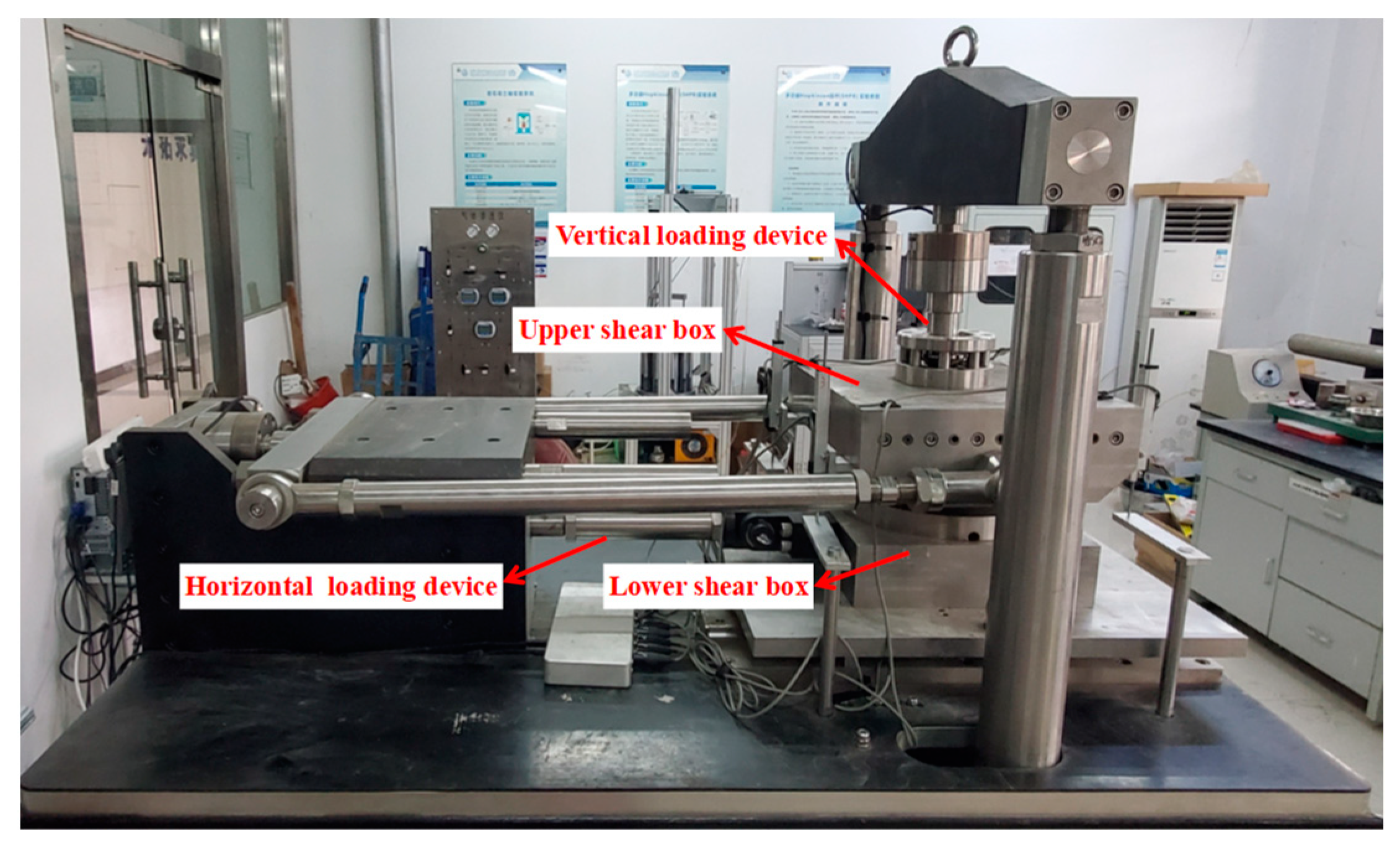
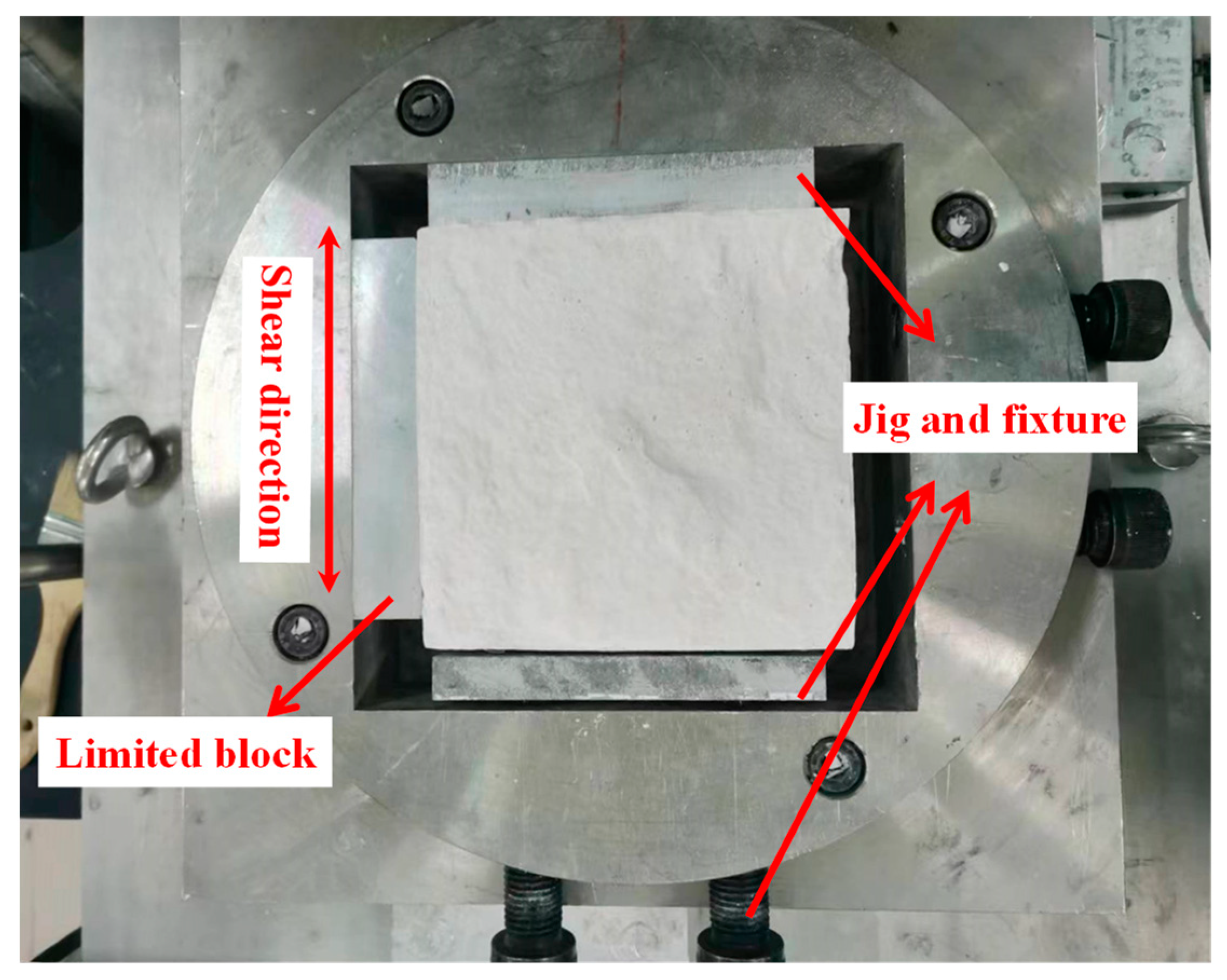
2.1. Test Apparatus

KTL–LADS150 (Figure 1) is a large-scale, direct shear system controlled by a motor. Axial and shear forces are provided by the motor actuator, without the need for pneumatic or hydraulic power devices. It can control the stress and strain in two directions. A maximum of 200 mm cube samples can be tested, and the maximum loading capacity is 150 kN. The test can be automatically loaded, and the data are collected and displayed through the keyboard or KTL–LAB software (version 2.0.1).

The test used a Geomagic Capture 3D noncontact laser scanner (Figure 2) provided by 3D Systems. The device is equipped with 3D blue light technology, a turntable, and a bracket that can scan 200 mm³-sized components, and the data capture rate is 985,000 points/time (0.3 s per scan). With a 0.060 mm accuracy, its resolution is 0.110 mm–0.180 mm, which meets the needs of rock joint morphology measurements.

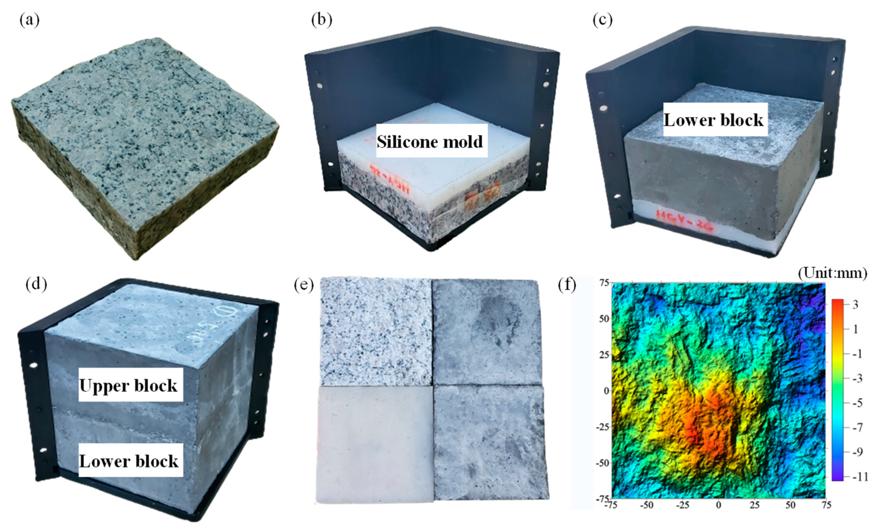
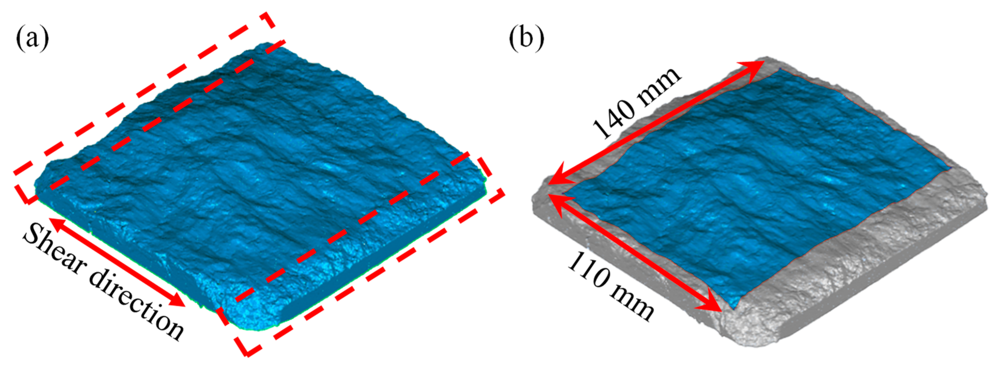
2.2. Specimen Preparation

To study the morphology degradation law of rock joints during cyclic shearing, the tested joint planes should have the same morphological characteristics. However, the morphology of natural rock joints is random and diverse, and it is difficult to obtain rock samples in batches that meet these requirements. The Brazilian splitting method is used to prepare the rock joints by pulling off specimens to form joint planes. The surface morphology of the joint surface obtained via this method is very similar to that of natural rock joints, and the production process is relatively simple. Therefore, a granite block with a size of 150 mm × 150 mm × 100 mm is selected for the Brazilian splitting test, a 150 mm × 100 mm plane is selected on the cuboid sample, and two marked lines are drawn in the direction of the long axis of the plane as the loading center of the splitting test. The rock block is placed in the middle of the loading device, with the upper and lower blades and the bearing plate placed in turn. Through the displacement control mode, the loading device is first controlled to only make contact with the bearing plate, and then a rate of 0.002 mm/s is applied until the rock cracks. An eccentric load should be avoided in the loading process, and finally, the rock joint surface is obtained. Then, through reverse manufacturing technology, liquid silicone is used to cast the rock joints into molds with natural morphologies (Figure 3b). In the laboratory, the joint samples are poured using grouting cement materials with fast-setting and high-strength characteristics, and the sample size is a 150 mm × 150 mm × 150 mm cube (Figure 3d). This method can replicate the joint morphology well, and samples can be produced in batches. Compared with the original rock joint, the morphology of the prepared joint sample has a smaller error. According to the methods suggested by the International Society for Rock Mechanics (ISRM 2007), uniaxial and triaxial compression tests are conducted on cylindrical samples with a diameter of 50 mm and a height of 100 mm to estimate the mechanical properties of the model material. The basic physico-mechanical parameters of the obtained artificial joint materials are shown in

Table 1. Physico-mechanical parameters of the joint specimens.

Model Material	Grouting Cement
Density (kg/m3)	2323
Young’s modulus (GPa)	11.54
Uniaxial compressive strength (MPa)	49.82
Cohesion (MPa)	18.94
Friction angle (°)	35.5
Poisson’s ratio	0.12

.

2.3. Test Conditions

The jig and fixture of the upper and lower parts of the shear box can clamp the sample tightly to limit its displacement and rotation in the cyclic shear process, and the limited block can keep the sample in the center of the shear box (Figure 4). Three kinds of constant normal loads (0.4, 1.0, and 2.5 MPa) [5] were tested. A 1/120 Hz sine wave was used until 6 mm of displacement was achieved, and the shear direction was reversed. To clearly show the wear process of the joint morphology during the cyclic shearing, a 20-cycle shear test process was divided into 8 stages, and the detailed test conditions are shown in

Table 2. Test conditions.

Sample Number	Normal Stress (MPa)	Frequency (Hz)	Shear Displacement (mm)	Cyclic Shear Number *
H1, H2, H3, H4, H5, H6, H7, and H8	2.5	1/120	6	1, 2, 3, 4, 5 10, 15, and 20
H9, H10, H11, H12, H13, H14, H15, and H16	1.0			1, 2, 3, 4, 5 10, 15, and 20
H17, H18, H19, H20, H21, H22, H23, and H24	0.4			1, 2, 3, 4, 5 10, 15, and 20

* Each sample number was tested against each cyclic shear number.

.

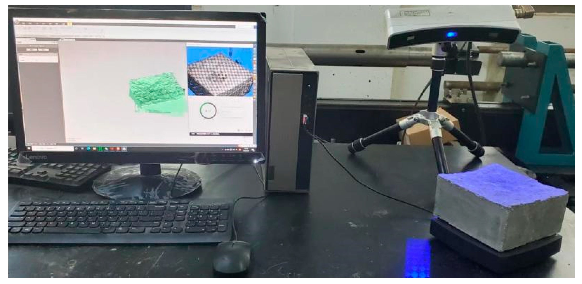
3. Characterization of 3D Joint Surfaces

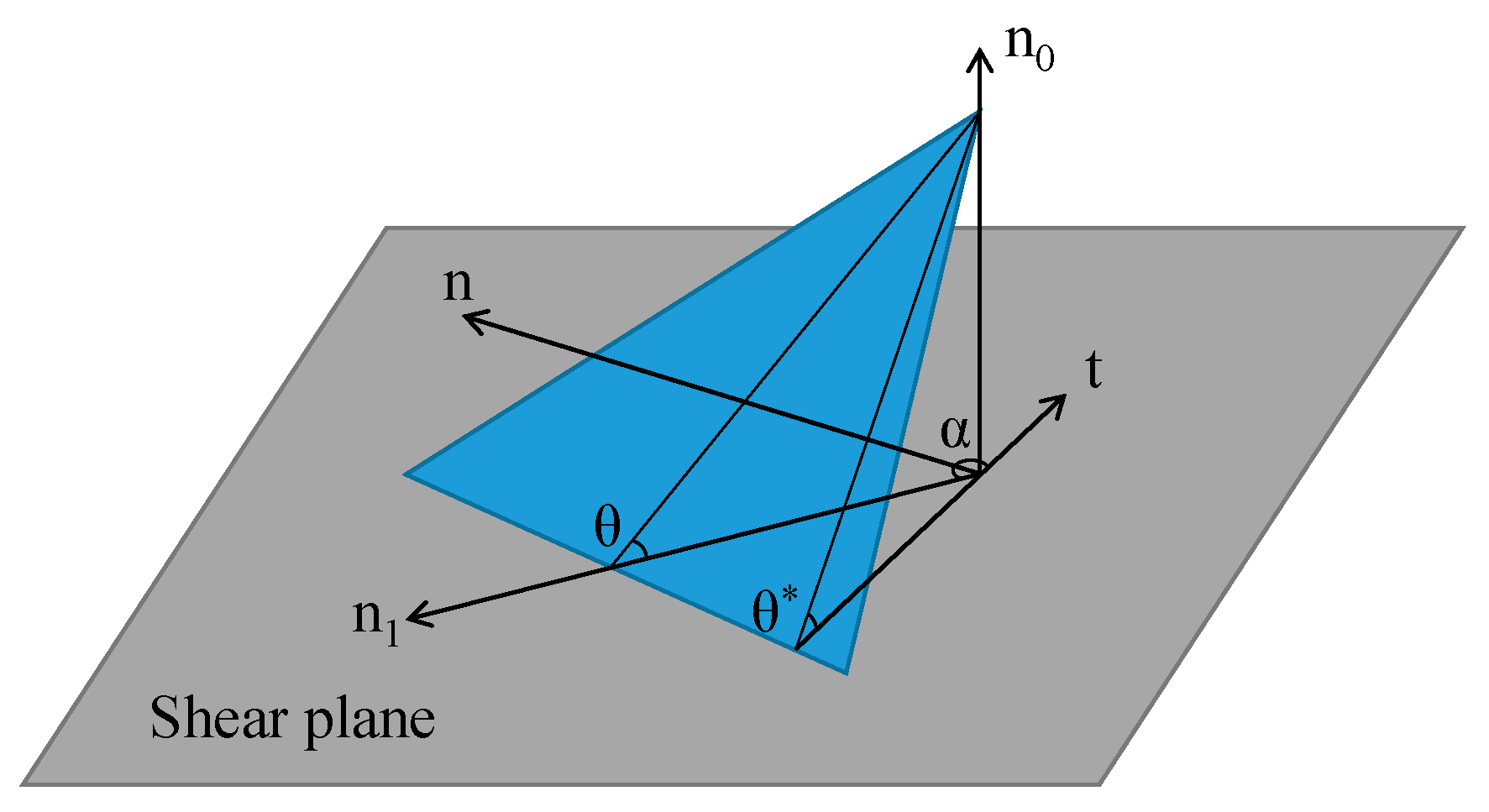
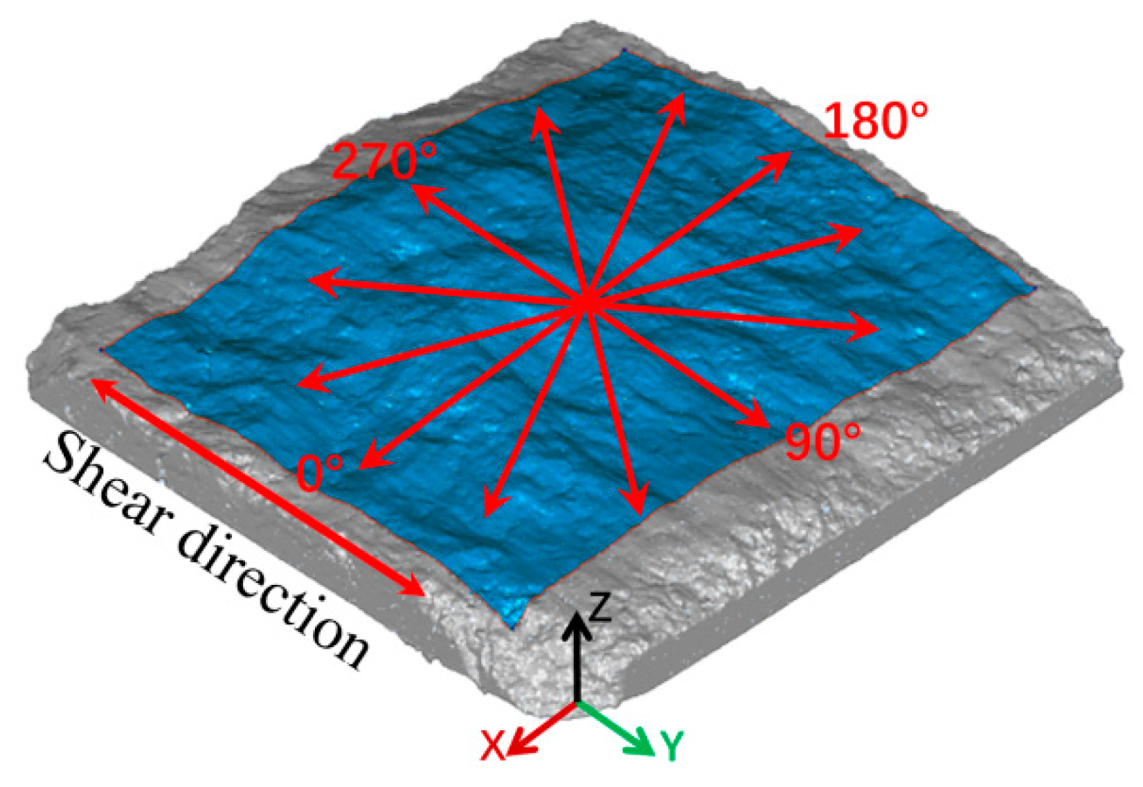
3.1. Joint Morphology Quantification

The joint roughness parameter is an important factor affecting the joint shear strength. Based on the methods described by Tatone and Grasselli [19,21], we carried out a test to quantitatively analyze the joint surfaces’ 3D morphology parameters before and after the cyclic shearing.

Grasselli used direct shear tests and found that the joint shear contact area is related to the shear direction and corresponding apparent dip angle, ${\theta }^{\ast }$ (Figure 5). The joint surface was discretized into triangular microelements, and the apparent dip angle ${\theta }^{\ast }$ was calculated as follows:

$$\tan {\theta }^{\ast }=-\tan \theta \cos \alpha$$

(1)

where $\theta$ is the angle between the shear plane and the triangular microelement, and $\alpha$ is the angle between the inclination of the triangular microelement and the shear direction (Figure 5).

The relationship between the total potential contact area $A_{{\theta }^{\ast }}$ and the apparent dip angle ${\theta }^{\ast }$ fits the following equation [19]:

$$A_{{\theta }^{\ast }}=A_0{\left(\frac{{\theta }_{max}^{\ast }-{\theta }^{\ast }}{{\theta }_{max}^{\ast }}\right)}^C$$

(2)

where $A_0$ is the maximum possible contact area in the shear direction calculated for a threshold angle of 0°; ${\theta }_{max}^{\ast }$ is the maximum apparent dip angle in the shear direction; and $C$ is a roughness parameter, calculated using a best-fit regression function.

Based on Grasselli’s theory, Tatone and Grasselli [21] evaluated the definite integral of Equation (2) between 0 and ${\theta }_{max}^{\ast }$, proving that $A_0{\theta }_{max}^{\ast }/\left(C+1\right)$ is a reasonable measure of roughness. The parameter $A_0{\theta }_{max}^{\ast }/\left(C+1\right)$ can be used as a representation of joint surface roughness, and it can reflect the joint surface roughness well. Moreover, this parameter has directivity and can be reasonably related to shear strength. Therefore, parameter $A_0{\theta }_{max}^{\ast }/\left(C+1\right)$ was adopted to evaluate the degradation of the joint surface roughness during the cyclic shear test.

3.2. Joint Surface Damage Calculation

After the cyclic shear test, the broken debris pieces were cleaned, and the 3D laser scanner was used to collect the surface morphology information of the joint lower block. Then, the point cloud data were packaged and processed.

During the first cycle of the shear test, the edge of the joint specimen near the maximum shear displacement formed a lost area due to the breakage, as shown in Figure 6a. This result is consistent with the observation made by Shen et al. [24,25]. The degradation of the joint morphology information in this area was caused by the boundary effect, so a quantitative analysis of the joint roughness degradation together with the inner area of the joint surface was not suitable. Hence, to eliminate the interference factors and reduce the test error, a 140 mm × 110 mm rectangular sampling window was cropped for a unified roughness calculation and an analysis area among all the testing samples, as illustrated in Figure 6b.

When the positive x axis is considered to be 0°, the roughness parameter $A_0{\theta }_{max}^{\ast }/\left(C+1\right)$ in each analyzed direction between 0° and 360° at an interval of 10° (counter-clockwise) can be calculated (Figure 7).

In addition, the lower block of each joint sample was photographed. The white area shows the wear and scratches caused by the cyclic shear, and the unworn area is surrounded by red curves. Both of these areas are depicted in Figure 8a, and they are consistent with Wang’s results [25].

The image binarization method was used to clearly distinguish the worn areas from the unworn areas. Then, the wear area ratio was calculated using the program, the formula for which can be expressed as follows:

$$r_w=A_w/A_t\times 100\%$$

(3)

where $A_w$ is the projection of the wear area, and $A_t$ is the projection of the joint surface (150 mm × 150 mm). An example of the image binarization calculation results is presented in Figure 8b.

4. Test Results and Discussion

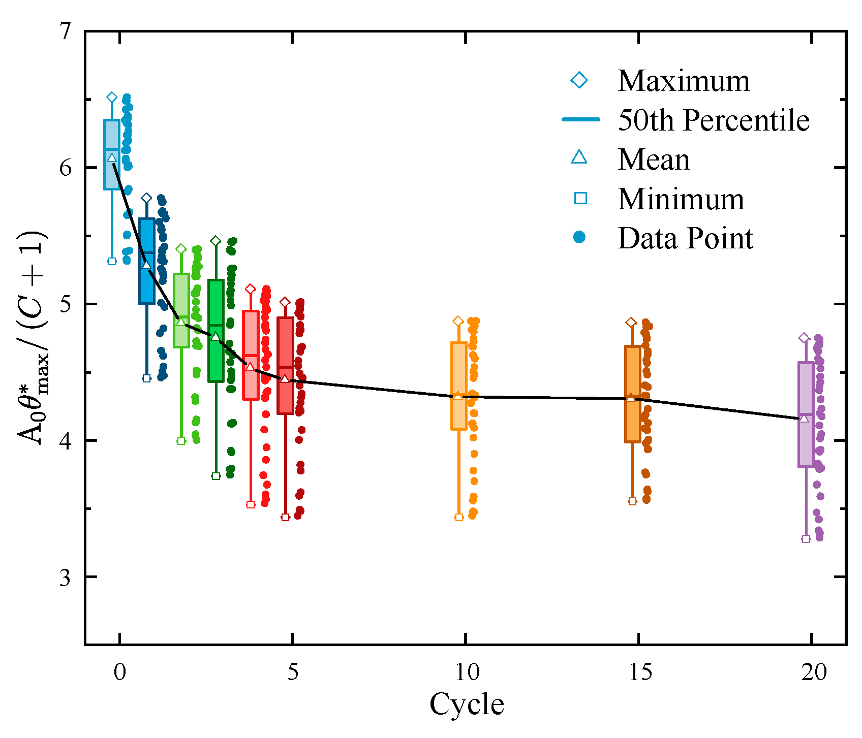
4.1. Degree of Surface Roughness Degradation

According to the angular convention, the shear directions were determined to be 90° and 270°. The polar plots of the 3D roughness parameter $A_0{\theta }_{max}^{\ast }/\left(C+1\right)$(Figure 9) present the calculated degree of the surface roughness degradation for the tested joint samples under different normal stress conditions. Figure 9 quantitatively illustrates the relative differences in the surface roughness along the 36 analyzed directions; the surface roughness decreased in all directions as the number of cycles increased. Taking every five cyclic shear cycles as intervals, the ratio of the variation in the roughness $A_0{\theta }_{max}^{\ast }/\left(C+1\right)$ at this interval to time was calculated in order to obtain the roughness degradation rate. It could be seen that the roughness degraded the fastest along the cyclic shear direction (90° and 270°) during the first five shear cycles (Figure 10). The intuitive prediction was that the roughness polar curve will shrink toward the origin. That is, it will gradually develop from an initial approximate circle to an ellipse, with the 0° direction as the long axis and the 90° direction as the short axis. In addition, the roughness degradation rate differed as the number of shear cycles increased under different normal stress conditions.

Using the Cartesian coordinate system to plot the roughness parameter curves can more clearly and intuitively show the degradation rate otherness of the joint surface roughness under different normal stress conditions. Figure 11a clearly shows that the roughness parameter $A_0{\theta }_{max}^{\ast }/\left(C+1\right)$ decayed approximately uniformly as the number of shear cycles increased with 0.4 MPa normal stress. The roughness was seriously attenuated after two shear cycles, and the degradation rate slowed down in the subsequent shearing process under 2.5 MPa normal stress (Figure 11c). The roughness degradation rate under 1.0 MPa normal stress (Figure 11b) was between these results.

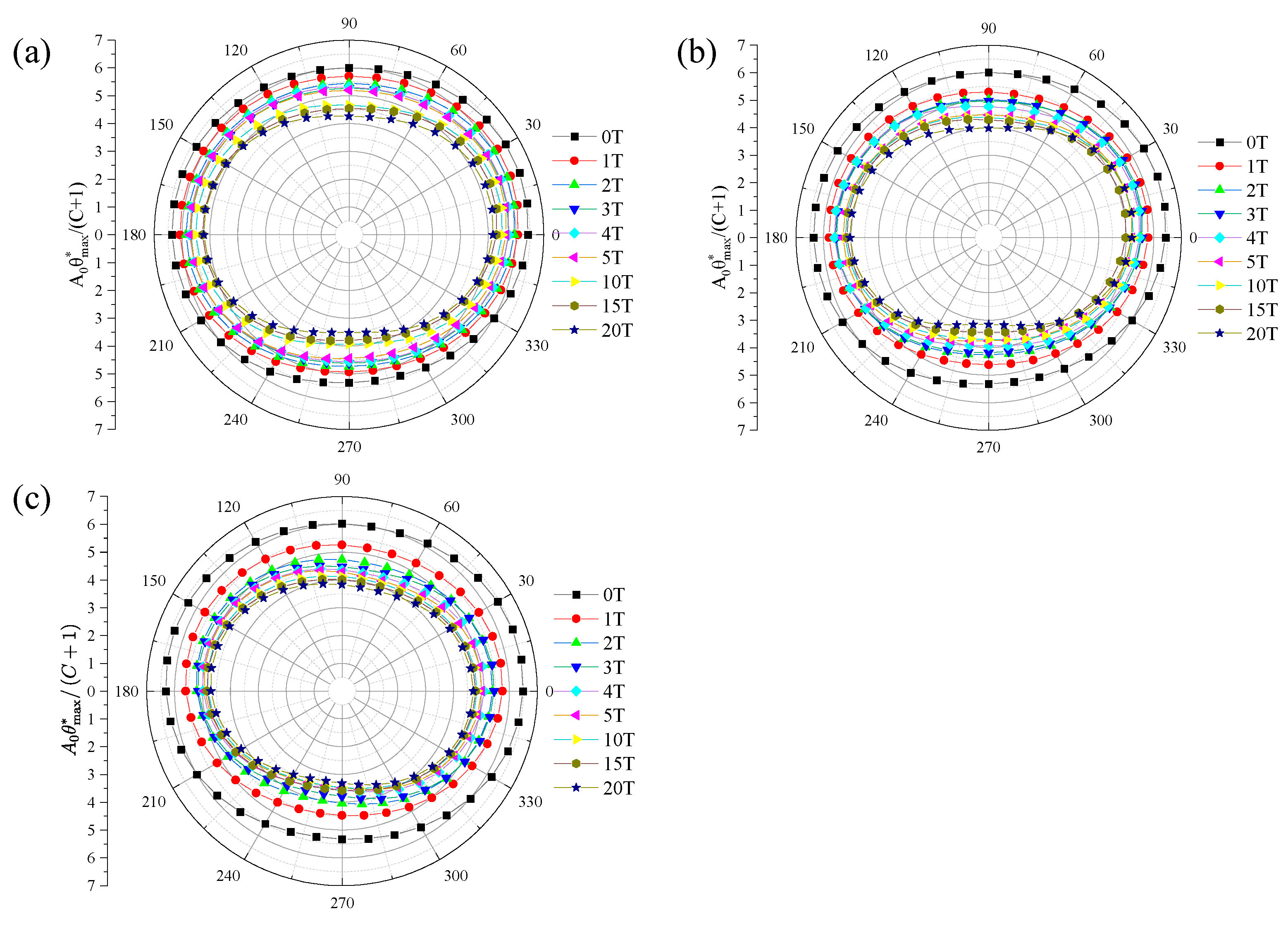
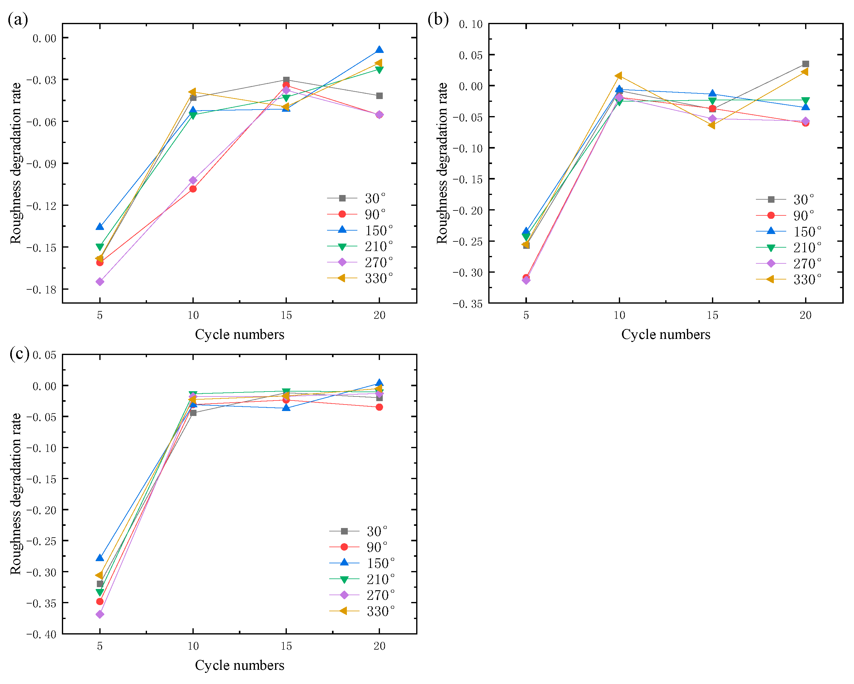
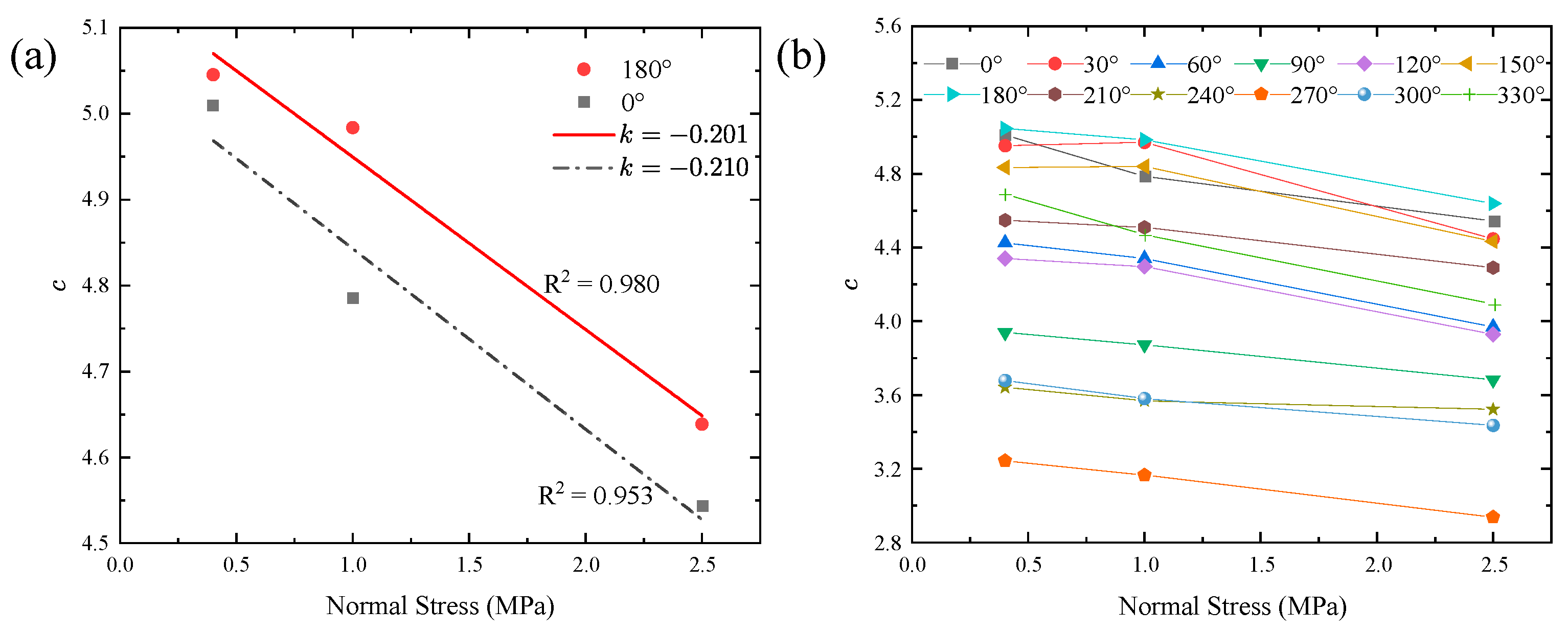
4.2. Surface Roughness Degradation Anisotropy

Taking the tests carried out under 2.5 MPa normal stress as an example, the statistical distribution of the roughness parameters in the 36 analyzed directions of the joint surface was illustrated with a box-and-whisker diagram (Figure 12). According to the statistical results, the maximum and mean of the roughness parameter $A_0{\theta }_{max}^{\ast }/\left(C+1\right)$ both declined as the number of shear cycles increased. Moreover, the degradation rate was first fast and then slow, and it tended to smooth after five shear cycles.

The interlocking asperities of joint surfaces may undergo tooth cutting, asperity wear, and debris backfilling during cyclic shearing. When the normal stress is larger, the degradation degree is greater, which leads to a rapid decrease in the micro-morphological parameters of the joint surface and a rapid degradation of the shear strength. In the subsequent cyclic shear process, the tooth-cutting, asperity wear, and debris-backfilling effects of the joint were obviously weakened, and the changes in the joint surface topography parameters tended to occur slowly.

In summary, two analyzed directions, those that were the most and least affected by cyclic shearing (the 90° to 270° and 0° to 180° analyzed directions, respectively), were selected for roughness parameter degradation anisotropy.

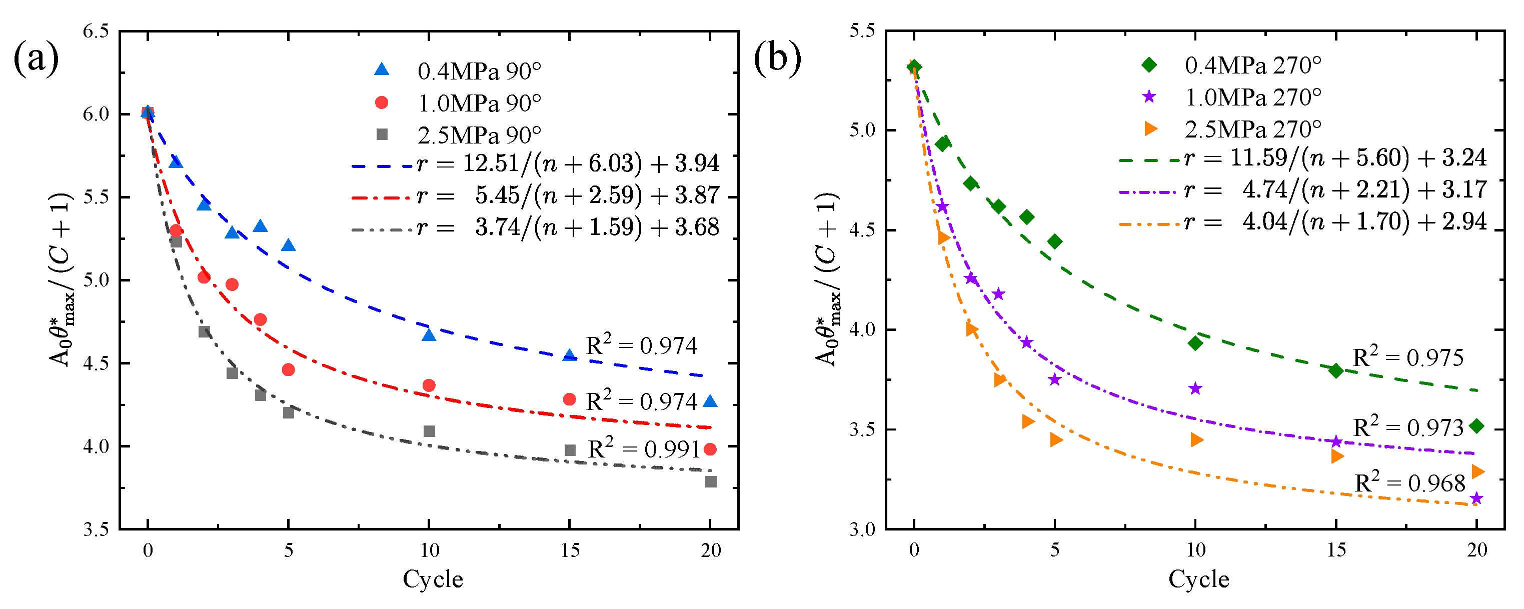
4.2.1. Analysis of the Roughness Degradation along the Shear Direction

Figure 13 shows the change process of the roughness parameter $A_0{\theta }_{max}^{\ast }/\left(C+1\right)$ along the shear direction (the 90° and 270° analyzed directions) during 20 cycles of shear testing under normal stresses of 0.4 MPa, 1.0 MPa, and 2.5 MPa. A roughness degradation trend the same as that shown in Figure 12 was observed, and the residual roughness parameters decreased as the normal stress increased.

To reveal the relationship between the number of shear cycles, normal stress, and surface roughness degradation, considering that roughness deterioration is a nonlinear process, a roughness degradation fitting formula (RDF) under cyclic shearing is proposed. The fitting formula can be rewritten as follows:

$$r=\frac{a}{n+b}+c$$

(4)

where $n$ is the number of shear cycles, $r$ is the joint roughness parameter $A_0{\theta }_{max}^{\ast }/\left(C+1\right)$, parameters $a$ and $b$ are factors related to the roughness degradation rates, and $c$ is the residual roughness when $n$ is large enough.

Fitting the test data plotted in Figure 13 shows that the RDF fit the relationship between the number of cyclic shears and the variation in the joint surface roughness. Furthermore, due to the anisotropy of the joint surface roughness, when an analyzed direction of the joint roughness was determined, parameters $a$, $b$, and $c$ had the relationship $a/b+c=r_0$ with the initial roughness $r_0$ (constant) of this analyzed direction.

Figure 14 shows that parameter $c$ decreased as the normal stress increased. These two factors followed a linear correlation, which is valid for predicting the residual roughness $c$ of joint surfaces after cyclic shears under different normal stresses.

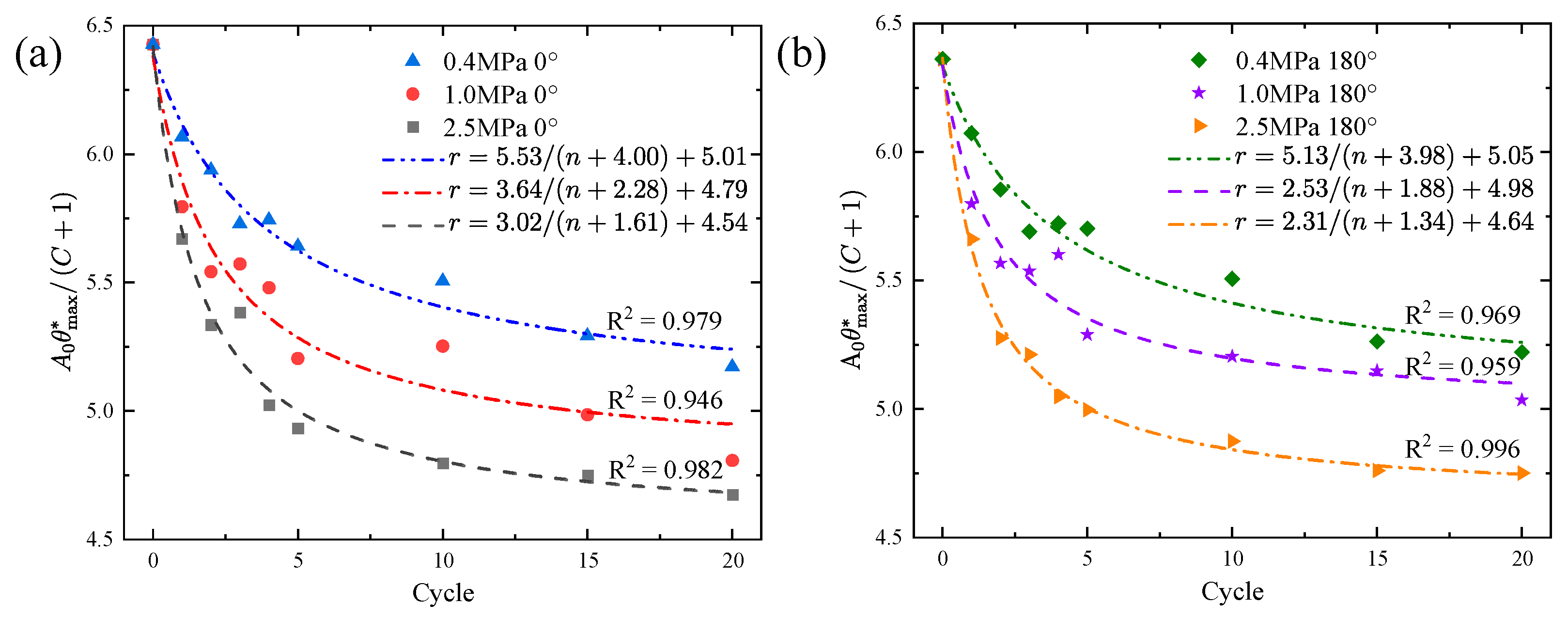
4.2.2. Analysis of the Roughness Degradation Perpendicular to the Shear Direction

Compared with the 90° and 270° analyzed directions, the 0° and 180° directions were the least affected by the cyclic shear. Figure 15 shows that the roughness degradation perpendicular to the shear direction was also consistent with the RDF, but the value of the residual roughness $c$ was generally larger than that along the shear direction.

Based on the RDF, considering the positive x axis to be 0°, the values of the residual roughness $c$ in each analyzed direction between 0° and 360° at intervals of 30° (counter-clockwise) could be calculated (Figure 16b). The results show that the roughness degradation degrees of the different analyzed directions in the cyclic shearing were inconsistent due to the joint surface roughness anisotropy. The roughness degradation degree was the most serious near the cyclic shear analyzed directions (240°, 270°, and 300°), and the influence was the smallest in the 0°, 30°, 150°, and 180° analyzed directions. A possible linear negative correlation was predicted between the residual roughness $c$ and the normal stress variation based on the fact that almost all of the analyzed directions decreased as the normal stress increased.

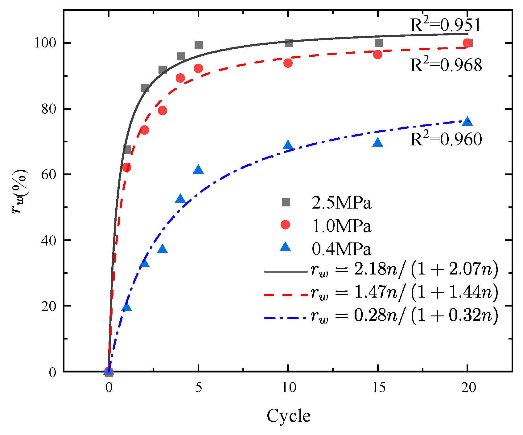
4.3. Analysis of the Joint Surface Wear

In the study conducted by Gui [26], the surface damage along the lower (vs. upper) surface had a relatively clearer degradation regularity. Hence, as described in Section 3.2, the image binarization method was used to process the top view of the lower block specimen’s surface after the cyclic shear in order to distinguish the worn areas (white) from the unworn areas (blue), and the wear area ratio $r_w$ was calculated. Figure 17 shows the wear process of the lower block specimen’s surface under 1.0 MPa. This process is consistent with Hong’s results [27].

As shown in Figure 18, the wear area ratio $r_w$ increased with the increase in the number of shear cycles, the increment rate of the wear area ratio $r_w$ slowed down after five shear cycles, and the value of $r_w$ was close to 100% under 2.5 MPa normal stress after five cycles. Figure 19 shows that asperity wear and debris backfill occurred during the first shear cycle. This result means that, during the subsequent shear cycles, the worn asperities on one side of the surface no longer had close occlusal contact with the hollows on the other side under a lower normal load. Evidently, the normal stress level plays a role in determining the asperity degradation on a joint surface, as mentioned by Xie [28] and Gentier [29]. Therefore, some partial areas of the lower joint surface were only slightly worn in the early stage of cyclic shearing. Under 0.4 MPa stress, even if more shear cycles are performed, the wear area ratio will not reach 100%.

A joint surface wear fitting formula under cyclic shear was proposed to reveal the relationship between the shear cycles, normal stress, and wear area ratio $r_w$. The fitting formula can be rewritten as follows:

$$r_w=\frac{k·n}{1+j·n} with r_w \in \left[0,1\right]$$

(5)

where $n$ is the number of shear cycles, $k$ is the first derivative value of the wear area ratio curve at point 0, and $k$ and $j$ follow an approximate linear correlation, as shown in Figure 20.

5. Conclusions

Under quasi-static conditions, cyclic shear tests were carried out to investigate the surface damage and roughness degradation of artificial rock joints with natural morphologies under different normal stresses. The 3D roughness parameters were measured and compared in 36 directions. The main conclusions are as follows:

• The polar plot of the 3D roughness parameter $A_0{\theta }_{max}^{\ast }/\left(C+1\right)$ of the joint surfaces analyzed in 36 directions demonstrates that, as the number of shear cycles increases, the polar curve of the joint surface roughness shrinks to the original direction. That is, it gradually develops from a circular to an elliptical shape, with the shear direction as the minor axis.
• The roughness degradation rate and the shear cycles are mutually interrelated with the normal stress level. A larger normal stress results in faster degradation rates and smaller residual roughness parameter values. The roughness degradation rate is approximately uniform with the shear cycles under low normal stress (0.4 MPa). When the normal stress increases, the roughness first degenerates quickly and then slowly.
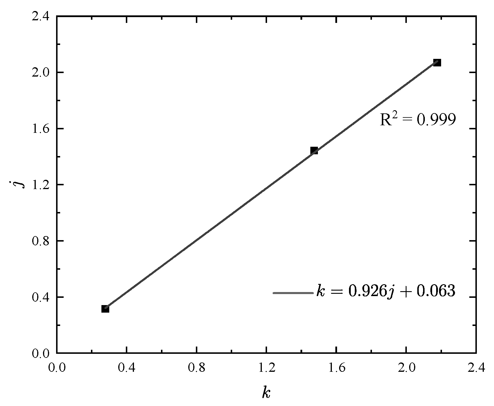
• Influenced by the cyclic shear direction, the 3D roughness of the joint surfaces degenerates anisotropically, and the most serious damage is sustained along the shear direction. An RDF ($r=a/\left(n+b\right)+c$) under cyclic shearing is proposed, and the residual roughness $c$ is linearly related to normal stress. The joint roughness after cyclic shears with different normal stresses can be predicted.
• The wear area ratio $r_w$ of the specimen’s lower block surfaces becomes severer as the number of shear cycles increases, and the increment rate of $r_w$ is first fast and then slow. A fitting formula of the joint surface wear under cyclic shearing is proposed, and it could aid in the assessment of the cumulative degree of wear in jointed rock masses.

References

1. Jing, L.; Stephansson, O.; Nordlund, E. Study of Rock Joints under Cyclic Loading Conditions. Rock Mech. Rock Eng. 1993, 26, 215–232. [Google Scholar] [CrossRef]
2. Huang, X.; Haimson, B.C.; Plesha, M.E. An investigation of the mechanics of rock joints—Part I. Laboratory investigation. Int. J. Rock Mech. Min. Sci. Geomech. Abstr. 1993, 30, 257–269. [Google Scholar] [CrossRef]
3. Kana, D.D.; Fox, D.J.; Hsiung, S.M. Interlock/friction model for dynamic shear response in natural jointed rock. Int. J. Rock Mech. Min. Sci. Geomech. Abstr. 1996, 33, 371–386. [Google Scholar] [CrossRef]
4. Fox, D.J.; Kana, D.D.; Hsiung, S.M. Influence of interface roughness on dynamic shear behavior in jointed rock. Int. J. Rock Mech. Min. Sci. 1998, 35, 923–940. [Google Scholar] [CrossRef]
5. Homand, F.; Belem, T.; Souley, M. Friction and degradation of rock joint surfaces under shear loads. Int. J. Numer. Anal. Methods Geomech. 2001, 25, 973–999. [Google Scholar] [CrossRef]
6. Lee, H.S.; Park, Y.J.; Cho, T.F. Influence of asperity degradation on the mechanical behavior of rough rock joints under cyclic shear loading. Int. J. Rock Mech. Min. Sci. 2001, 38, 967–980. [Google Scholar] [CrossRef]
7. Jafari, M.K.; Hosseini, K.A.; Pellet, F. Evaluation of shear strength of rock joints subjected to cyclic loading. Soil Dyn. Earthq. Eng. 2003, 23, 619–630. [Google Scholar] [CrossRef]
8. Xiao-Ming, Z.; Li, H.B.; Bo, L. Study of mechanical characteristics of simulated rock joints with second-order asperity under cyclic shear loading. Rock Soil Mech. 2014, 35, 371–379. [Google Scholar]
9. Mirzaghorbanali, A.; Nemcik, J.; Aziz, N. Effects of Cyclic Loading on the Shear Behaviour of Infilled Rock Joints Under Constant Normal Stiffness Conditions. Rock Mech. Rock Eng. 2014, 47, 1373–1391. [Google Scholar] [CrossRef]
10. Liu, B.; Li, H.B.; Liu, Y.Q. Experimental study of deformation behavior of rock joints under cyclic shear loading. Rock Soil Mech. 2013, 34, 2475. [Google Scholar]
11. Xu, B.; Liu, X.R.; Zhou, X.H. Investigation on the macro-meso fatigue damage mechanism of rock joints with multiscale asperities under pre-peak cyclic shear loading. Soil Dyn. Earthq. Eng. 2021, 151, 16. [Google Scholar] [CrossRef]
12. Dang, W.G.; Konietzky, H.; Fruhwirt, T. Cyclic Frictional Responses of Planar Joints Under Cyclic Normal Load Conditions: Laboratory Tests and Numerical Simulations. Rock Mech. Rock Eng. 2020, 53, 337–364. [Google Scholar] [CrossRef]
13. Ferrero, A.M.; Migliazza, M.; Tebaldi, G. Development of a New Experimental Apparatus for the Study of the Mechanical Behaviour of a Rock Discontinuity Under Monotonic and Cyclic Loads. Rock Mech. Rock Eng. 2010, 43, 685–695. [Google Scholar] [CrossRef]
14. Greenwood, J.A. A Unified Theory of Surface-Roughness. Proc. R. Soc. Lond. Ser. A-Math. Phys. Eng. Sci. 1984, 393, 133–157. [Google Scholar]
15. Mulvaney, D.J.; Newland, D.E. Identification of surface-roughness. Proc. Inst. Mech. Eng. Part C-J. Mech. Eng. Sci. 1985, 199, 281–286. [Google Scholar] [CrossRef]
16. Barton, N. Review of a new shear-strength criterion for rock joints. Eng. Geol. 1973, 7, 287–332. [Google Scholar] [CrossRef]
17. Belem, T.; Homand-Etienne, F.; Souley, M. Quantitative parameters for rock joint surface roughness. Rock Mech. Rock Eng. 2000, 33, 217–242. [Google Scholar] [CrossRef]
18. Grasselli, G.; Egger, P. Constitutive law for the shear strength of rock joints based on three-dimensional surface parameters. Int. J. Rock Mech. Min. Sci. 2003, 40, 25–40. [Google Scholar] [CrossRef]
19. Grasselli, G. Manuel Rocha Medal recipient - Shear strength of rock joints based on quantified surface description. Rock Mech. Rock Eng. 2006, 39, 295–314. [Google Scholar] [CrossRef]
20. Sun, F.T.; Jiang, Q.R.; She, C.X. Research on Three-dimensional Roughness Characteristics of Tensile Granite Joint. In Proceedings of the International Conference on Civil, Architectural and Hydraulic Engineering (ICCAHE 2012), Zhangjiajie, China, 10–12 August 2012. [Google Scholar]
21. Tatone, B.S.; Grasselli, G. A method to evaluate the three-dimensional roughness of fracture surfaces in brittle geomaterials. Rev. Sci. Instrum. 2009, 80, 125110. [Google Scholar] [CrossRef]
22. Chen, S.J.; Zhu, W.C.; Yu, Q.L. Characterization of Anisotropy of Joint Surface Roughness and Aperture by Variogram Approach Based on Digital Image Processing Technique. Rock Mech. Rock Eng. 2016, 49, 855–876. [Google Scholar] [CrossRef]
23. Tang, H.M.; Ge, Y.F.; Wang, L.Q. Study on Estimation Method of Rock Mass Discontinuity Shear Strength Based on Three-Dimensional Laser Scanning and Image Technique. J. Earth Sci. 2012, 23, 908–913. [Google Scholar] [CrossRef]
24. Shen, H.; Liu, Y.; Li, H. Rate-Dependent Characteristics of Damage and Roughness Degradation of Three-Dimensional Artificial Joint Surfaces. Rock Mech. Rock Eng. 2022, 55, 2221–2237. [Google Scholar] [CrossRef]
25. Wang, G.; Zhang, X.P.; Jiang, Y.J. Rate-dependent mechanical behavior of rough rock joints. Int. J. Rock Mech. Min. Sci. 2016, 83, 231–240. [Google Scholar] [CrossRef]
26. Gui, Y.; Xia, C.; Ding, W. A New Method for 3D Modeling of Joint Surface Degradation and Void Space Evolution Under Normal and Shear Loads. Rock Mech. Rock Eng. 2017, 50, 2827–2836. [Google Scholar] [CrossRef]
27. Hong, E.-S.; Kwon, T.-H.; Song, K.-I. Observation of the Degradation Characteristics and Scale of Unevenness on Three-dimensional Artificial Rock Joint Surfaces Subjected to Shear. Rock Mech. Rock Eng. 2015, 49, 3–17. [Google Scholar] [CrossRef]
28. Xie, H.P.; Wang, J.A.; Xie, W.H. Fractal effects of surface roughness on the mechanical behavior of rock joints. Chaos Solitons Fractals 1997, 8, 221–252. [Google Scholar] [CrossRef]
29. Gentier, S.; Riss, J.; Archambault, G. Influence of fracture geometry on shear behavior. Int. J. Rock Mech. Min. Sci. 2000, 37, 161–174. [Google Scholar] [CrossRef]
Figure 1. Cyclic shear apparatus.
Applsci 13 01441 g001
Figure 2. Schematic diagram of a joint surface measured using the 3D scanner.
Applsci 13 01441 g002
Figure 3. Schematic diagram of the joint sample preparation process: (a) preparing a single joint rock specimen, (b) using silicone to replicate the joint surface, (c) casting the lower block, (d) casting the upper block, (e) comparing the casting results, (f) scanning the sample’s surface morphology.
Applsci 13 01441 g003
Figure 4. Sample fixed in shear box.
Applsci 13 01441 g004
Figure 5. Schematic of the apparent dip angle.
Applsci 13 01441 g005
Figure 6. Measuring of the joint surface morphology via 3D scanning: (a) lost area due to breakage, (b) uniform roughness calculation and analysis area.
Applsci 13 01441 g006
Figure 7. Schematic diagram of the analyzed directions of the roughness parameter.
Applsci 13 01441 g007
Figure 8. (a) Surface wear area and scratches of specimen H3 after cyclic shear. (b) The image binarization method was used to distinguish the worn area from the unworn area.
Applsci 13 01441 g008
Figure 9. Polar plots of the 3D roughness parameter, A 0 θ m a x / ( C + 1 ) , of the lower joint surface under different normal stresses: (a) 0.4 MPa, (b) 1.0 MPa, and (c) 2.5 Mpa.
Applsci 13 01441 g009
Figure 10. Plots of the roughness parameter, A 0 θ m a x / ( C + 1 ) , degradation rate of the lower joint surface under different normal stresses: (a) 0.4 MPa, (b) 1.0 MPa, and (c) 2.5 Mpa.
Applsci 13 01441 g010
Figure 11. Direct coordinate system of the 3D roughness parameter, A 0 θ m a x / ( C + 1 ) , of the lower joint surface under different normal stresses: (a) 0.4 MPa, (b) 1.0 MPa, and (c) 2.5 MPa.
Applsci 13 01441 g011
Figure 12. Box-and-whisker plot of the statistical roughness parameter for cyclic sheared joints under 2.5 MPa.
Applsci 13 01441 g012
Figure 13. Roughness parameter change process along the cyclic shear directions under different normal stresses: (a) 90° and (b) 270° analyzed directions.
Applsci 13 01441 g013
Figure 14. Curves of parameter c vs. normal stress along the 90° and 270° analyzed directions.
Applsci 13 01441 g014
Figure 15. Roughness parameter change process along cyclic shear directions under different normal stresses: (a) 0° and (b) 180° analyzed directions.
Applsci 13 01441 g015
Figure 16. Curves of parameter c vs. normal stress: (a) 0° and 180° analyzed directions, (b) analyzed direction between 0° and 360° at an interval of 30°.
Applsci 13 01441 g016
Figure 17. Using the image binarization method to process the worn (white area) and unworn areas (blue area) of the surface under 1.0 MPa.
Applsci 13 01441 g017
Figure 18. Curves of worn area ratio r w vs. shear cycles.
Applsci 13 01441 g018
Figure 19. Local damage evolution under low normal stress.
Applsci 13 01441 g019
Figure 20. Curves of parameters k vs. j in the joint surface wear fitting formula.
Applsci 13 01441 g020