Featured Application
The guidance of uncrewed aerial/ground vehicles, high-end security, surveillance, and various 3D manipulation, inspection, and measurements.
Abstract
Applying edge preservation filters for cost aggregation has been a leading technique in generating dense disparity maps. However, traditional approaches usually require intensive calculations, and their design parameters must be tuned for different scenarios to obtain the best performance. This paper shows that a simple texture-independent aggregation approach can achieve similar high performance. The proposed algorithm is equivalent to a sequence of matrix multiplications involving two weighting matrices and a primary matching cost. Notably, the weighting matrices are constant for image pairs with the same resolution. For higher matching accuracy, we integrate the algorithm with a multi-scale scheme to fully exploit the spatial distribution of textures in the image pairs. The resultant hybrid approach is efficient and accurate enough to surpass most existing approaches in stereo matching. The performance of the proposed approach is verified by extensive simulation results using the Middlebury (3rd Edition) benchmark stereo database.
1. Introduction
Binocular stereo matching aims to restore 3D information based on a pair of rectified 2D images obtained from the same scene. Due to its passive and low-cost sensing characteristics, the acquired depth information may play a vital role in the guidance of uncrewed aerial/ground vehicles, high-end security, surveillance, and various 3D manipulation, inspection, and measurement applications.
Traditional stereo matching algorithms can be categorized into global and local algorithms [1], depending on the extent of information used for matching evaluation. Local methods consider only neighboring pixels for each candidate pixel, while the other methods exploit the entire image information. Traditional matching algorithms normally begin with formulating a stereo matching cost that estimates the matching degree between reference patches and target patches.
Global stereo matching algorithms require computationally demanding optimization algorithms, such as graph cuts [2] and dynamic programming [3,4], to find the disparity of each pixel. To facilitate the algorithms in real time, [5] implemented an integrated scheme combining a dynamic programming algorithm and a local algorithm using a graphics processing unit (GPU), while [6] implemented semi-global stereo matching using a field-programmable gate array (FPGA).
Unlike global algorithms, the stereo matching cost of local and non-local/semi-global algorithms is an aggregation of primary matching costs. The aggregation is normally conducted as a filtering procedure, and the resultant disparity map is obtained through the winner-take-all (WTA) strategy [1]. Since the computational complexities of local algorithms are usually smaller than that of other algorithms, they are widely used in practical applications.
Among the early efforts of using filters for cost volume aggregation in local algorithms, the matching performance of [7] was constrained by a fixed supporting window. This shortage was alleviated in [8] by introducing an adaptive window-size approach. Later, the Guided Image Filtering (GIF) model [9] was successfully implemented in [10], which demonstrates an edge-preserving advantage. Based on [9,11] further proposed a weighted guided image filter (WGIF) scheme to avoid halo artifacts and was used in [12] for disparity estimation. As the matching performance of GIF depends on the size of kernel windows, [13] proposed an adaptive guided filtering method to exclude pixels that do not belong to the same region. Besides, an iterative guided filtering approach [14] and an adaptive support weight version [15] were created to improve matching accuracy. More recently, [16] proposed weights according to structural features and filtered the matching cost volume by using the adaptive guided filtering method proposed by [13]. These are typical local stereo matching algorithms that do not aggregate matching costs outside the supporting window.
In [17], matching costs were aggregated according to tree structures individually derived from the entire image pair. Similarly, matching algorithms based on the so-called permeability filter [18] and pervasive guided image filtering [19] can effectively aggregate matching costs based on the whole image. In addition [20], integrated multi-scale information into the scheme of [19], significantly improving the matching performance. These algorithms use the full window for aggregation and are called non-local stereo matching algorithms. To solve the problem of matching ambiguity in low-texture areas and high sensitivity in high-texture areas [21], proposed the use of both the local support window and the whole image.
In addition to these traditional algorithms, disparity maps can also be computed using deep learning-based methods. These algorithms have the advantage of high matching accuracy. For instance [22], developed an automatic encoder to generate feature maps for semi-global stereo matching, and [23] implemented an unsupervised disparity estimation neural network based on the principle of disparity consistency. Besides [24], proposed a simplified independent component correlation algorithm (ICA)-based local similarity stereo matching algorithm to further improve matching accuracy in non-texture areas and boundaries. Among the deep learning-based methods, both [25,26] are typical end-to-end stereo matching networks, which realize the aggregation of matching costs through 3D convolution operations.
However, as pointed out in [27], compared with traditional stereo matching algorithms, deep learning-based stereo matching algorithms still suffer from insufficient generalization ability. Additionally, they typically require GPU-based computing resources. The current characteristics of deep learning-based methods justify continued research on traditional methods.
In most traditional local and non-local stereo matching algorithms, the weights for the matching cost aggregation depend on the texture of the image pair. This dependency restricts the possibility of sharing weights for different scenes. To improve the computational efficiency of stereo matching, this paper proposes a texture-independent aggregation method.
The main contributions of this paper are as follows:
- (1)
- We propose an aggregation algorithm for stereo matching that significantly simplifies computation without sacrificing matching performance. The aggregation weights can be shared between different scene images with the same resolution.
- (2)
- To provide a higher matching accuracy, we integrate the algorithm with a multi-scale scheme to exploit the spatial distribution of texture that can achieve improved performance with a minor increase in computational efforts.
2. Methods
2.1. Traditional Local and Non-Local Stereo Matching Algorithms
In this section, we examine two representative stereo matching algorithms proposed in [9,17], which are classified as local and non-local, respectively.
Traditional local and non-local stereo matching algorithms start with calculating a primary matching cost that reflects the degree of match between corresponding pixels on an image pair. Many measurements can be used for computing the primary matching cost. The implementation presented in this paper uses a linear combination of the truncated absolute difference of the gradient, denoted as and the Hamming distance of the census transform:
where q is the location of a pixel, d is the estimated disparity of this pixel, and are the left and right images, respectively, and are the gradients of this pixel in the horizontal and vertical directions, respectively, represents the Census transformation [28], and Ham is the Hamming Distance computation. Left and right images often appear different at the same location due to lighting conditions and image sensing inhomogeneity. These two matching costs are adopted because they can significantly reduce the misleading effects of pixel-level intensity variations.
To consider both matching costs, we make a linear combination of and to obtain the primary matching cost, :
where is a weighting constant. It is set to be 0.95 in the following investigations.
The primary matching cost can be further aggregated to include information from surrounding pixels. The aggregation of the primary matching cost is the most crucial step that affects the stereo matching performance. A general form of the aggregated matching cost, denoted as , can be written as
where is the supporting region centered at p, and is the aggregation weight. For the well-celebrated algorithms based on the weighted guided image filter, such as those proposed in [10,12,16], the aggregation weight, denoted as , can be represented in the following form:
where and represent the mean value and variance operations, respectively, and is a small constant introduced to avoid division by zero. From (4), we know that is closely related to the patterns on . Besides, depends on the spatial distribution of the image since its value is a function of the interaction between two regions which are centered at p and q, denoted as and .
In [17], the matching cost values are aggregated based on the minimum spanning tree (MST) being derived from the guidance image, where the aggregation weight, denoted as , is calculated as
where is a path determined by the MST between a pixel pair located at p and q, u and v are the coordinates of pixels in the path, and is a shaping parameter. It is clear from (5) that also depends on the patterns on .
Once we have the aggregated matching cost, the estimated disparity map, denoted as , can be obtained by the winner-take-all computation:
where and are the lower and upper bounds of disparity, assumed to be known beforehand.
Based on the above examination and derivation, we know that the aggregation weights of [9,17] are related to the texture and spatial distance of the participating pixels on an image pair. Different scene images have different aggregation weights, making the weights not sharable. This shortcoming is typical for most local and non-local stereo matching algorithms.
2.2. The Proposed Aggregation Method
We propose conducting a texture-independent cost aggregation scheme in three steps. In the first step, we consider the matching cost continuity in the horizontal direction. Then we enforce the vertical continuity of the cost in the second step. In each of these two steps, the aggregation is derived based on the minimization of an objective function. In the third step, we integrate the proposed algorithm with a cross-scale scheme to provide higher matching accuracy and efficient computation simultaneously.
2.2.1. The First Step: Horizontal Aggregation
In the first step, the proposed aggregation cost assumes the least squared difference from the primary matching cost. In addition, the cost has fewer differences with the horizontal 2 neighbors of each pixel. Based on these assumptions, we compose an objective function to be minimized:
where is the proposed aggregation cost to be defined in the first step, M and N are the vertical and horizontal resolutions of , is a normalization factor, and is a set of 2 horizontal neighbors of the pixel under consideration, as depicted in Figure 1. In the figure, the coordinates of pixels are expended as and This 2-neighbor regularization term limits the abrupt changes in the horizontal direction of the proposed aggregation cost.
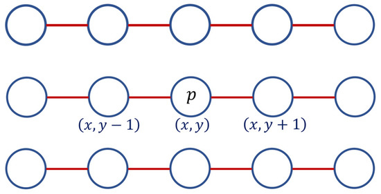
Figure 1.
A pixel located at p and its two horizontal neighbors, denoted as .
The aggregated matching cost in this step is constrained only in the horizontal direction, being independent in the vertical direction. We assume the objective function can be decomposed into M independent objective functions of the rows:
where
In minimizing each of the objective function , we may take partial derivative of it with respect to :
This results in the following N equations for different y:
If we define
Equation (11) can be written in a matrix form as
Besides, with (12) we observe that:
Taking the whole image into consideration, (13) becomes
The matrix is tridiagonal, symmetric, and sparse. This N-by-N matrix is invertible for positive [29]. From (15), we may obtain the proposed aggregated matching cost, , by inverting :
This procedure has the advantage that the matching cost can be calculated using a simple linear combination with constant weights while the resultant matching cost has a small difference with the horizontal neighborhoods, and only a smooth transition in this direction is possible.
2.2.2. The Second Step: Vertical Aggregation
Similar to the first step, we can create an objective function, denoted as , for an aggregated matching cost, The function applies constraints in the vertical direction while enforces its least squared difference from the matching cost aggregated in the first step, :
We assume the objective function is composed of sub-functions , which are mutually independent in the horizontal direction. can be solved by taking a partial derivative of with respect to in each column. By accumulating the results through the whole image, we have
where
Again, the matrix is an M-by-M invertible tridiagonal sparse matrix for positive [29]. Combining (18) and (16), and considering that is symmetric, we have
From (20), we know that the aggregation of the primary matching cost can be simplified as a series of matrix multiplication. The horizontal aggregation weight, , and the vertical aggregation weight, , are constant tridiagonal matrices of the parameter . Their inverses can be calculated beforehand once the image sizes, M and N, are known. Under this condition, the computational complexity of the proposed algorithm is much simpler than most aggregation approaches.
Taking M = 480, N = 720, and as an example, Figure 2 and Figure 3 show visualized representations of in two and three dimensions. It can be seen from these figures that the values of the matrix are mostly concentrated near the diagonal. It can be clearly seen that the values of the points on both sides of the diagonal gradually decrease as the distance from the diagonal increases. The behavior of is similar to that of .
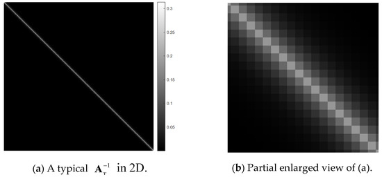
Figure 2.
Two-dimensional visualization of a typical (M = 480, N = 720, and ), where lighter colors represent higher values. (a) is the entire matrix and (b) is a partial view of (a) with the length enlarged by a factor of 16.
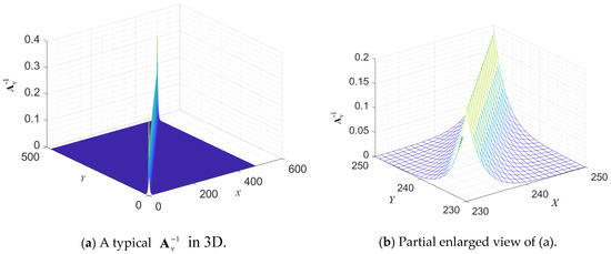
Figure 3.
Three-dimensional visualization of a typical (M = 480, N = 720, and ). Component values are expressed as heights.
As is symmetric and sparse, its element values in the row and column directions follow the same pattern. For a fixed image size, is completely defined by the only parameter . Figure 4 demonstrates the element values of as a function of . The image size is also 480-by-720, and only elements on row 240 are depicted.
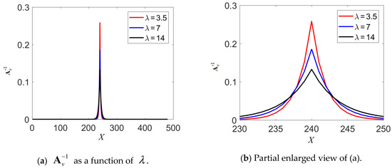
Figure 4.
as a function of . The image size is 480-by-720. The plots show the element values of on row 240. (a) The value of for different values. (b) Partial enlargement of (a).
Also, as observed in Figure 4, the distribution of the sparse matrix becomes smoother when is larger, which implies a larger effective range of the aggregation. When is smaller, the distribution of the sparse matrix is sharper, and the effective range of the matching cost aggregation is smaller. This observation is consistent with (7) and (17) that, when the value of is larger, the objective functions, and , have stronger constraints on the aggregated matching costs, and .
From the above analysis, we have gathered that the effective range of and is similar to the size of the aggregation window or the length of an aggregation path in the local and non-local algorithms. For images with larger resolutions, a larger value of is required to effectively aggregate the matching cost in a broader range. For images with smaller resolutions, a smaller value of is more adequate.
2.2.3. The Proposed Scheme: Integration of the Texture-Independent Scheme with a Cross-Scale Cost Aggregation Algorithm
To enhance the matching accuracy of the cost aggregation algorithm derived in the last section, we present its integration with a cross-scale scheme of [20,30] in this section. This hybrid approach is recommended since higher matching accuracy can be achieved with only a slight increase in computation. Similarly, other algorithms can be integrated with the proposed scheme.
The cross-scale scheme of [20,30], denoted as CS, considers the primary matching costs of various scales. The scheme begins with down-sampling an image pair into K pairs. For each image pair, a matching cost is calculated according to (20). We denote the matching cost of the k-th pair as , , where K is the highest pair with the lowest resolution. The framework is derived by introducing an objective function for the cross-scale scheme of [20,30]:
where is a constant constraining factor and is the aggregation window centered at p. For K = 2 and = 1.5, minimizing (21) with respect to results in a simple representation that the aggregated matching cost of the zero-layer is
where is the number of pixels within the aggregation window . As can be observed in the original scheme [20,30], the larger the value of K, the more multi-scale features the aggregated matching cost contains. The larger the value of , the larger the proportion of down-sampled information in the aggregation matching cost, and vice versa.
A primary disparity map can be obtained using the winner-take-all principle:
To reduce the noise effects on , we create an updated cost volume based on the primary disparity map of (23):
where is the erroneous region detected via the left-right consistency examination. Implementation details of (21), (22), and (24) can be found in [20]. Finally, we aggregate the updated cost volume using the algorithm of (20):
This is the final aggregated matching cost. We can then obtain the final disparity map by applying the winner-take-all computational principle to once again.
3. Results
To investigate the matching performance of the proposed scheme, performance comparisons have been made between eight representative stereo matching schemes and the proposed scheme:
- End-to-end real-time stereo matching network proposed in [25], denoted as RTSMNet.
- Matching algorithm based on a combination of the adaptive support weight with iterative guided filter and the sum of gradient matching [15], denoted as ISM.
- Sparse representation over a learned discriminative dictionary for stereo matching [4], denoted as DDL.
- Stereo matching algorithm based on two-phase adaptive optimization of ad-census and gradient fusion [8], denoted as TPAO.
- Stereo matching algorithm based on per pixel difference adjustment, iterative guided filter, and graph segmentation [14], denoted as IGF.
- Local stereo matching using adaptive cross-region-based guided image filtering with orthogonal weights [16], denoted as ACR-GIF-OW.
- Hierarchical guided-image-filtering for stereo matching [20], denoted as HGIF.
- Stereo matching with fusing adaptive support weights [21], denoted as FASW.
- The proposed scheme, which is an integration with a cross-scale cost aggregation algorithm as described in the last section.
We selected several stereo image pairs from the Middlebury version 3 [31] and the KITTI Vision Benchmark Suite [32] datasets for demonstration. The “trainingQ” of the Middlebury version 3 [31] dataset is composed of 15 groups of pictures from “Adirondack” to “Vintage”. As summarized in Table 1, resolutions of the images are around 480-by-720.

Table 1.
Resolution of the images for stereo matching.
According to the previous section’s discussion, the design parameter is positively related to the image resolution under matching. In the following demonstrations, the values of are simply assigned as
Figure 5 shows the disparity maps obtained by these stereo matching algorithms on four of the image sets. Table 2 and Table 3 present the error rates and weighted error rates of the algorithms using the complete “trainingQ” of the Middlebury version 3 [31] dataset. In the tables, the experimental results of the four algorithms for comparison are obtained from the original literature. For ease of viewing, the graphical representations of Table 2 and Table 3 are shown in Figure 6 and Figure 7.
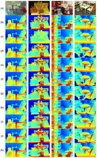
Figure 5.
Visual comparison of disparity maps obtained by different algorithms. (a) The left scene images selected from the Middlebury version 3 [31] dataset (from left to right): Adirondack, Jadeplant, Playroom, and Playtable. (b) Ground-truth disparity maps, (c) Disparity maps generated by RTSMNET [25]. (d) Disparity maps generated by ISM [15]. (e) Disparity maps generated by DDL [4]. (f) Disparity maps generated by TPAO [8]. (g) Disparity maps generated by IGF [14]. (h) Disparity maps generated by ACR-GIF-OW [16]. (i) Disparity maps generated by HGIF [20]. (j) Disparity maps generated by FASW [21]. (k)Disparity maps generated by an integration of the proposed scheme.
Table 2.
Comparison of the error rates in the non-occluded region without refinements using different matching algorithms (%). In calculating the error rates, the error threshold = 1.0.
Table 3.
Comparison of the error rates in the all-region without refinement (%). In calculating the error rates, the error threshold = 1.0. The best score for each image set is highlighted in bold.
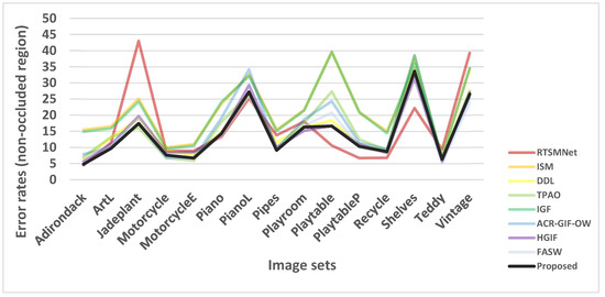
Figure 6.
Comparison of the error rates in the non-occluded region. This diagram is a graphical representation of Table 2.
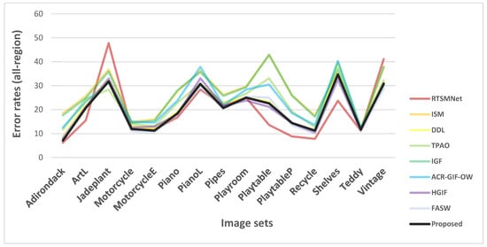
Figure 7.
Comparison of the error rates in the all-region. This diagram is a graphical representation of Table 3.
The performance of FASW [21] and the proposed algorithm are more prominent for stereo matching on the dataset. Specifically, in the non-occluded region, the proposed algorithm has the lowest mismatch rate, followed by FASW [21] and the HGIF [20] algorithm. In the all-region, the RTSMNet [25] algorithm has the lowest mismatch rate, followed by FASW [21] and the proposed algorithm.
However, we can observe a significant performance deterioration in using RTSMNet [25] to predict the disparity maps of the “Jadeplant” and “Vintage” image sets. RTSMNet [25] is a deep learning-based method, its generalization ability depends on the quality and richness of the training dataset. Similar scenes may be rare in its training set. This behavior is not observed in traditional algorithms because their performance is less sensitive to scene type.
The time required for the matching of a rectified stereo image pair for each algorithm is summarized in Table 4. These computations were executed in MATLAB 2017b using an Intel Core I5 8300 H and 16 GB RAM. Notably, the proposed algorithm takes the least computational time. If we consider both matching accuracy and algorithmic complexity, the proposed algorithm is close to the best accuracy while requiring the least amount of computation.
Table 4.
Comparison of the running time of each algorithm for a pair of rectified images (s). These computations were executed in MATLAB 2017b using an Intel Core I5 8300H and 16 GB RAM.
To verify the stereo matching performance of the proposed algorithm in real scenes, the autonomous driving training dataset of KITTI Vision Benchmark Suite [32] is used for further demonstration. The dataset contains 194 image pairs with corresponding ground truth disparity maps. Performance comparisons to be presented are between the following stereo matching schemes:
- Stereo matching based on adaptive guided filtering [13], denoted as AGF.
- Adaptive stereo matching using tree filtering [17], denoted as MST.
- The ISM algorithm [15].
- The HGIF algorithm [20].
- The FASW algorithm [21].
- The proposed scheme.
Figure 8 shows the disparity maps generated by these algorithms on the KITTI suite [32]. Each algorithm performs stereo matching on 194 sets of stereo image pairs. Due to space constraints, we only select three stereo-image pairs for visual comparison. Table 5 shows the quantitative matching performance of these algorithms. Four scores are compared: the percentage of erroneous pixels in non-occluded areas, denoted as Non-Occ (%); the percentage of erroneous pixels in all regions, denoted as All (%); the average disparity error in terms of pixel numbers in non-occluded areas, denoted as Non-Occ (pixels); and the average disparity error in terms of pixel numbers in all regions, denoted as All (pixels). The scores used for comparison are quoted from [21].
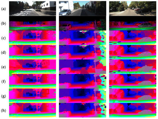
Figure 8.
Visual comparison of disparity maps obtained by different algorithms using the KITTI Vision Benchmark Suite [32]. (a) Three of the left scene images selected from the dataset. (b) Ground-truth disparity maps. (c) Disparity maps generated by ISM [15]. (d) Disparity maps generated by AGF [13]. (e) Disparity maps generated by MST [17]. (f) Disparity maps generated by HGIF [20]. (g) Disparity maps generated by FASW [21]. (h) Disparity maps generated by the proposed scheme.
Table 5.
Comparison of the effects of each algorithm using the KITTI image dataset.
As seen from Figure 8 and Table 5, compared with the five representative aggregation methods, the proposed algorithm outperforms other algorithms in items Non-Occ (%), All (%), and Non-Occ (pixels), with scores of 6.30%, 7.48%, and 1.3 pixels, respectively. Its performance is only slightly inferior to [21] on All (pixels), with a score of 1.58, which is higher than [21]’s 1.45.
Figure 9 shows three disparity maps generated by the proposed algorithm using three sets of multi-view remote sensing images (pictures from https://github.com/whuwuteng/benchmark_ISPRS2021, accessed on 15 February 2019). These additional disparity maps demonstrate the effectiveness of the proposed approach.
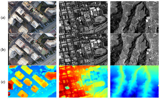
Figure 9.
Disparity maps of remote sensing images. (a) Left image of the scene (b) Right image of the scene (c) Disparity maps obtained by the proposed algorithm.
4. Discussion
Traditional local and non-local stereo matching algorithms require an efficient aggregation procedure, which is the most critical stage for generating accurate dense disparity maps. The aggregation weights in most stereo matching algorithms in the literature, unfortunately, are scenario specific.
We re-examined the procedure of cost aggregation from the perspective of matrix operations and treated the aggregation as constraining the degree of difference between adjacent costs. By decoupling the aggregation procedure in the horizontal and vertical directions, we propose a new aggregation algorithm to effectively calculate a cost volume for stereo matching. This process is equivalent to multiplying the initial cost by two constant matrices.
The aggregation algorithm requires two constant weight matrices that are only related to the image resolution and can be calculated beforehand. These matrices are mathematically proven to be independent of image texture and thus can be applied to different scene images of the same resolution. This algorithm can be used for integration with other schemes to provide both computational efficiency and stereo matching accuracy. We demonstrate its integration with the cross-scale scheme of [20,30].
Through numerical experiments using indoor and outdoor benchmark stereo image datasets, we demonstrate that the integrated scheme is not only computationally efficient but also provides disparity maps that are highly comparable to the most accurate algorithms in the literature.
In the future, we will focus on real-time implementation of the proposed algorithm by using, for instance, GPU-based systems. Preprocessing techniques, such as the algorithm proposed in [33] for detecting and removing shadows, can be employed to further improve the accuracy of dense disparity maps.
Author Contributions
Conceptualization, Y.-Z.C. and C.Z.; methodology, C.Z. and Y.-Z.C.; software, C.Z.; validation, Y.-Z.C. and C.Z.; formal analysis, C.Z.; investigation, Y.-Z.C.; resources, Y.-Z.C. and C.Z.; data curation, C.Z.; writing—original draft preparation, C.Z.; writing—review and editing, Y.-Z.C.; visualization, C.Z.; supervision, Y.-Z.C.; project administration, Y.-Z.C.; funding acquisition, Y.-Z.C. All authors have read and agreed to the published version of the manuscript.
Funding
This research was funded by National Science and Technology Council, Taiwan, grant number 110-2221-E-182-034 and 111-2221-E-182-057; and Chang Gung Memorial Hospital, grant number CORPD2J0041 and CORPD2J0042.
Institutional Review Board Statement
Not applicable.
Informed Consent Statement
Not applicable.
Data Availability Statement
Data sharing not applicable. The Middlebury version 3 datasets are available at https://vision.middlebury.edu/stereo/data/scenes2014/. The KITTI Vision Benchmark Suite datasets are available at https://www.cvlibs.net/datasets/kitti/. The multi-view remote sensing images are available at https://github.com/whuwuteng/benchmark_ISPRS2021. These datasets were accessed on 15 February 2019.
Conflicts of Interest
The authors declare no conflict of interest.
Nomenclature
| a constant matrix used in deriving the proposed aggregation cost of the first step consisting of the parameter λ. | |
| a constant matrix used in deriving the proposed aggregation cost of the second step consisting of the parameter λ. | |
| B | a matrix consisting of elements of . |
| the general form of an aggregated matching cost. | |
| an updated disparity cost volume to reduce the noise effects in images. | |
| the final aggregated matching cost that integrates the proposed algorithm with a cross-scale cost aggregation scheme described in [20,30]. | |
| the primary matching cost used in this paper. | |
| the proposed aggregation cost defined in the first step. | |
| the proposed aggregation cost defined in the second step. | |
| a matching cost calculated by the Hamming distance of the census transform. | |
| the matching cost of the k-th scale layer, each aggregated by the proposed scheme. | |
| the estimated matching cost of the k-th scale layer, each aggregated by an integrated scheme consisting of the proposed scheme and a cross-scale cost aggregation algorithm described in [20,30]. | |
| a matching cost calculated by the truncated absolute difference of the gradient. | |
| D | a matrix consisting of elements of . |
| d | the estimated disparity of a pixel. |
| the disparity map based on an image pair. | |
| a function to calculate the Hamming Distance. | |
| an independent objective function of image rows. | |
| , | the left and right images, respectively. |
| an objective function for the cross-scale scheme proposed in [20,30]. | |
| , | objective functions representing the least squared difference between the proposed aggregation cost and the primary matching cost in the horizontal and vertical directions, respectively. |
| K | the number of pairs in the cross-scale cost aggregation. Each image pair is down-sampled from the original pair. |
| L | a path determined by the minimum spanning tree technique [17]. |
| M | the vertical resolution of . |
| min | a function to calculate the minimum value between several amounts. |
| N | the horizontal resolution of . |
| a set of 2 horizontal neighbors. | |
| p, q | the location of a pixel. The symbols are interchangeably used as parameters. |
| the Census transformation. | |
| an independent objective function of image columns. | |
| the general form of aggregation weights. | |
| the aggregation weight of the weighted guided image filter. | |
| the aggregation weight based on the minimum spanning tree technique [17]. | |
| Greek symbols | |
| α | a weighting constant. |
| β | a shaping parameter. |
| γ | a constraining factor. |
| ε | a small constant introduced to avoid division by zero. |
| λ | a normalization factor. |
| μ | the mean value function. |
| the variance function. | |
| Ω | the supporting region centered at a pixel. |
| Mathematical Operator | |
| , | the gradients of intensity in the horizontal and vertical directions, respectively. |
References
- Scharstein, D.; Szeliski, R. A taxonomy and evaluation of dense two-frame stereo correspondence algorithms. Int. J. Comput. Vis. 2002, 47, 7–42. [Google Scholar] [CrossRef]
- Boykov, Y.; Veksler, O.; Zabih, R. Fast approximate energy minimization via graph cuts. IEEE Trans. Pattern Anal. Mach. Intell. 2001, 23, 1222–1239. [Google Scholar] [CrossRef]
- Hirschmuller, H. Stereo processing by semiglobal matching and mutual information. IEEE Trans. Pattern Anal. Mach. Intell. 2008, 30, 328–341. [Google Scholar] [CrossRef]
- Yin, J.; Zhu, H.; Yuan, D.; Xue, T. Sparse representation over discriminative dictionary for stereo matching. Pattern Recognit. 2017, 71, 278–289. [Google Scholar] [CrossRef]
- Hallek, M.; Boukamcha, H.; Mtibaa, A.; Atri, M. Dynamic programming with adaptive and self-adjusting penalty for real-time accurate stereo matching. J. Real-Time Image Proc. 2022, 19, 233–245. [Google Scholar] [CrossRef]
- Lu, Z.; Wang, J.; Li, Z.; Chen, S.; Wu, F. A Resource-Efficient Pipelined Architecture for Real-Time Semi-Global Stereo Matching. IEEE Trans. Circuits Syst. Video Technol. 2022, 32, 660–673. [Google Scholar] [CrossRef]
- Yoon, K.J.; Kweon, I.S. Adaptive support-weight approach for correspondence search. IEEE Trans. Pattern Anal. Mach. Intell. 2006, 28, 650–656. [Google Scholar] [CrossRef]
- Liu, H.; Zhang, H.; Nie, X.; He, W.; Luo, D.; Jiao, G.; Chen, W. Stereo matching algorithm based on two-phase adaptive optimization of AD-Census and gradient fusion. In Proceedings of the Conference on Real-time Computing and Robotics, Xining, China, 15–19 July 2021; pp. 726–731. [Google Scholar]
- He, K.; Sun, J.; Tang, X. Guided image filtering. IEEE Trans. Pattern Anal. Mach. Intell. 2013, 35, 1397–1409. [Google Scholar] [CrossRef]
- Hosni, A.; Rhemann, C.; Bleyer, M.; Rother, C. Fast cost-volume filtering for visual correspondence and beyond correspondence search. IEEE Trans. Pattern Anal. Mach. Intell. 2013, 35, 504–511. [Google Scholar] [CrossRef]
- Li, Z.; Zheng, J.; Zhu, Z.; Yao, W.; Wu, S. Weighted guided image filtering. IEEE Trans. Image Process. 2014, 24, 120–129. [Google Scholar]
- Hong, G.S.; Kim, B.G. A local stereo matching algorithm based on weighted guided image filtering for improving the generation of depth range images. Displays 2017, 49, 80–87. [Google Scholar] [CrossRef]
- Yang, Q.; Ji, P.; Li, D.; Yao, S.; Zhang, M. Fast stereo matching using adaptive guided filtering. Image Vis. Comput. 2014, 32, 202–211. [Google Scholar] [CrossRef]
- Hamzah, R.A.; Ibrahim, H.; Hassan, A.H.A. Stereo matching algorithm based on per pixel difference adjustment, iterative guided filter and graph segmentation. J. Vis. Commun. Image Represent. 2017, 42, 145–160. [Google Scholar] [CrossRef]
- Hamzah, R.A.; Kadmin, A.F.; Hamid, M.S.; Ghani, S.F.A.; Ibrahim, H. Improvement of stereo matching algorithm for 3D surface reconstruction. Signal Process. Image Commun. 2018, 65, 165–172. [Google Scholar] [CrossRef]
- Kong, L.; Zhu, J.; Ying, S. Local stereo matching using adaptive cross-region-based guided image filtering with orthogonal weights. Math. Probl. Eng. 2021, 2021, 1–20. [Google Scholar] [CrossRef]
- Yang, Q. Stereo matching using tree filtering. IEEE Trans. Pattern Anal. Mach. Intell. 2015, 37, 834–846. [Google Scholar] [CrossRef]
- Çı˘gla, C.; Alatan, A.A. An efficient recursive edge-aware filter. Signal Process. Image Commun. 2014, 29, 998–1014. [Google Scholar] [CrossRef]
- Zhu, C.; Chang, Y.Z. Efficient stereo matching based on pervasive guided image filtering. Math. Probl. Eng. 2019, 2019, 3128172. [Google Scholar] [CrossRef]
- Zhu, C.; Chang, Y.Z. Hierarchical guided-image-filtering for efficient stereo matching. Appl. Sci. 2019, 9, 3122. [Google Scholar] [CrossRef]
- [Wu, W.; Zhu, H.; Yu, S.; Shi, J. Stereo matching with fusing adaptive support weights. IEEE Access 2019, 7, 61960–61974. [Google Scholar]
- Nguyen, V.D.; Nguyen, H.V.; Jeon, J.W. Robust stereo data cost with a learning strategy. IEEE Trans. Intell. Transp. Syst. 2017, 18, 248–258. [Google Scholar] [CrossRef]
- Godard, C.; Aodha, O.M.; Brostow, G.J. Unsupervised monocular depth estimation with left-right consistency. In Proceedings of the Conference on Computer Vision and Pattern Recognition (CVPR), Honolulu, HI, USA, 21–26 July 2017; pp. 6602–6611. [Google Scholar]
- Chen, S.; Zhang, J.; Jin, M. A simplified ICA-based local similarity stereo matching. Vis. Comput. 2021, 37, 411–419. [Google Scholar] [CrossRef]
- Chang, J.R.; Chen, Y.S. Pyramid stereo matching network. In Proceedings of the Conference on Computer Vision and Pattern Recognition (CVPR), Salt Lake City, UT, USA, 19–21 June 2018; pp. 5410–5418. [Google Scholar]
- Xie, Y.; Zheng, S.; Li, W. Feature-guided spatial attention upsampling for real-time stereo matching network. IEEE MultiMedia. 2021, 28, 38–47. [Google Scholar] [CrossRef]
- Tian, M.; Yang, B.; Chen, C.; Huang, R.; Huo, L. HPM-TDP: An efficient hierarchical PatchMatch depth estimation approach using tree dynamic programming. ISPRS 2019, 155, 37–57. [Google Scholar] [CrossRef]
- Zabih, R.; Woodfill, J. Non-parametric local transforms for computing visual correspondence. In Proceedings of the Third European Conference on Computer Vision, Stockholm, Sweden, 2–6 May 1994; pp. 151–158. [Google Scholar]
- Venetis, I.E.; Kouris, A.; Sobczyk, A.; Gallopoulos, E.; Sameh, A. A direct tridiagonal solver based on Givens rotations for GPU architectures. Parallel Comput. 2015, 49, 101–116. [Google Scholar] [CrossRef]
- Zhang, K.; Fang, Y.; Min, D.; Sun, L.; Yang, S.; Yan, S.; Tian, Q. Cross-scale cost aggregation for stereo matching. In Proceedings of the IEEE Conference on Computer Vision and Pattern Recognition, Columbus, OH, USA, 23-28 June 2014; pp. 1590–1597. [Google Scholar]
- Scharstein, D.; Hirschmüller, H.; Kitajima, Y.; Krathwohl, G.; Nesic, N.; Wang, X.; Westling, P. High-resolution stereo datasets with subpixel-accurate ground truth. In Proceedings of the German Conference on Pattern Recognition (GCPR 2014), Münster, Germany, 12–15 September 2014; pp. 1–12. [Google Scholar]
- Moritz, M.; Geiger, A. Object Scene Flow for Autonomous Vehicles. In Proceedings of the Conference on Computer Vision and Pattern Recognition (CVPR), Boston, MA, USA, 8–10 June 2015; pp. 1–10. [Google Scholar]
- Rani, E.F.I.; Pushparaj, T.L.; Raj, E.F.I. Escalating the resolution of an urban aerial image via novel shadow amputation algorithm. Earth Sci. Inform. 2022, 15, 905–913. [Google Scholar] [CrossRef]


Disclaimer/Publisher’s Note: The statements, opinions and data contained in all publications are solely those of the individual author(s) and contributor(s) and not of MDPI and/or the editor(s). MDPI and/or the editor(s) disclaim responsibility for any injury to people or property resulting from any ideas, methods, instructions or products referred to in the content. |
© 2023 by the authors. Licensee MDPI, Basel, Switzerland. This article is an open access article distributed under the terms and conditions of the Creative Commons Attribution (CC BY) license (https://creativecommons.org/licenses/by/4.0/).