Abstract
The Cedaya-S340 Holgutu Highway Construction Project is located in the Mongolian Autonomous Prefecture of Bayingolin in the Xinjiang Uygur Autonomous Region. It is an important traffic channel that connects Luntai County and Hejing County at the southern foot of Tianshan Mountains. As the major component of the highway project, the Huola Mountain Tunnel has a sharp topographic relief, and, therefore, commonly used land geophysical detection instruments cannot work on it. Therefore, we conducted a qualitative survey on the ground-to-air and airborne electromagnetic detection methods used at the Huola Mountain Tunnel site to provide basic data for the design of highway tunnels. The geophysical survey summarized the ground–airborne frequency-domain electromagnetic method (GAFEM) and the helicopter-borne time-domain electromagnetic method (HTEM) developed by Jilin University, and measured 15 measuring lines. Apparent resistivity imaging was performed for each section, and the results were consistent. This study comprehensively analyzed the apparent resistivity profile and geological mapping data. Then, the study inferred the major stratigraphic boundaries, fault fracture zones, rock fragmentation, weakness, karst development, and water content in accordance with background value, low-resistivity anomaly shape, low-resistivity anomaly value, and gradient value in the apparent resistivity profile. Finally, the study identified the scope of two main low-resistivity anomalies, located at the tunnel entrance and exit, respectively, which are basically consistent with the known fault location. The results of this study show that on the basis of the apparent resistivity maps of GAFEM and HTEM, the overall distribution law is basically consistent with site landform, hydrogeology, tectonic geology, and aerial image data. The results provide guidance for the construction of the Huola Mountain Tunnel and ensure the construction safety and progress of the tunnel.
1. Introduction
Airborne and ground–airborne electromagnetic methods are geophysical exploration techniques that use aircraft as the carrier. They exhibit high speed, good accessibility, and high efficiency; additionally, they are particularly suitable for conducting geological survey on complex terrain conditions (e.g., mountains, deserts, forest covers, lakes, and swamps) [,].
Compared with the fixed-wing time-domain electromagnetic system, the helicopter-borne time-domain electromagnetic method (HTEM) demonstrates strong maneuverability and high resolution [,]. Therefore, most airborne electromagnetic surveys use HTEM systems. For the helicopter time-domain aviation system, we fixed the transmitting and receiving coils on the pod. The Earth was excited to generate a secondary induction field through the large transmitting magnetic moment generated by the transmitting coils on the pod, and the coil sensor received the secondary field signal. The conductivity information of the subsurface structure was obtained by analyzing and interpreting the secondary field-induced voltage signal []. At present, many types of helicopter pod time-domain airborne electromagnetic detection systems have been developed internationally, some of which are mature, such as the VTEM system by Geotech [], the AeroTEM system by Aeroquest [], the HeliGEOTEM system by Fugro [], the HoistEM system by GPX, the SkyTEM system by Hoes University in Denmark [,,], and the CHTEM system by Jilin University of China and the Center for Aerogeophysical Remote Sensing of Land and Resources [,]. These systems have been successfully applied to the exploration of mineral deposits in most parts of the world, with exploration depth reaching 300–500 m [,].
The ground–airborne electromagnetic method uses ground transmission and air reception [,]. Given the separate transceiver system, this method exhibits the advantages of rapid noncontact measurement by the airborne electromagnetic method, high-power transmission by the ground electromagnetic method, and deep detection; it has developed rapidly in recent years [,]. At present, internationally mature ground–airborne electromagnetic detection systems include the Terra Air system in Canada, the FLAIRTEM system in Australia, the GREATEM system in Japan [], the DESMEX system in Germany [], and the GAFEM system in China [,]. The Terra Air and FLAIRTEM systems use large-loop magnetic sources for transmission. This feature exhibits the disadvantages of a small magnetic moment and a limited detection depth range. To solve these problems, the GREATEM, DESMEX, and GAFEM systems use grounding wire (electrical source) as their emission source. Scientists have used the GREATEM system to investigate the geoelectric structure of the Bandai volcanic area in northeastern Japan. The maximum detection depth of the system can reach 800 m []. Lin et al. (2019) [] obtained the electrical structure within a depth of 2.5 km below the surface of Leshan Town, Changchun by using the GAFEM system; however, the result suffered from the problem of low resolution in the shallow area. At present, there are many resistivity imaging methods, such as apparent resistivity imaging [,,] and layered resistivity inversion [,], but there is no research on joint resistivity imaging using HTEM and GAFEM airborne electromagnetic detection data.
The Huola Mountain Tunnel is located near Cedaya Township, Luntai County, the Mongolian Autonomous Prefecture of Bayingolin. The total length of this tunnel is 8520 m; hence, it is a very long tunnel with a maximum buried depth of 1291.2 m. The tunnel site is located on a medium to high mountain landform, with steep mountains on both sides of the entrance and exit. At present, the tunnel site area does not experience traffic conditions. Therefore, we conducted helicopter-borne and ground–airborne electromagnetic survey in the Huola Mountain Tunnel section to solve the problems of difficult access for ground personnel and large tunnel burial depth. The construction of the tunnel has not yet started. This is a preconstruction assessment, and the objective is to realize fast, deep, and detailed exploration of the tunnels, obtain subsurface geological structures along the exploration line, and provide basic data for highway tunnel design.
2. Overview of the Survey Area
The Cedaya-S340 Holgutu Highway Construction Project is located in the Mongolian Autonomous Prefecture of Bayingolin, Xinjiang Uygur Autonomous Region (Figure 1). It is an important traffic channel that connects Luntai County and Hejing County at the southern foot of Tianshan Mountains in Bayingolin. It is also an important tourism highway in the Xinjiang Uygur Autonomous Region. The Cedaya-S340 Holgutu Highway directly or indirectly connects the G3012 Expressway, S340, G314, G218, and other trunk highways. The construction of this highway will further improve the regional road network, particularly its traffic conditions and transport efficiency. Simultaneously, the Cedaya-S340 Holgutu Highway opens the southward corridor of the famous scenic spot Bayanbulak Grassland, considerably shortening driving distance from Bayanbulak to Korla and Luntai and playing an important role in promoting the development of the tourism industry in Bayingolin [,]. The Huola Mountain Tunnel, as the major control of the highway project (black box area in Figure 1), is located near Cedaya Township, Luntai County, Bayingolin.
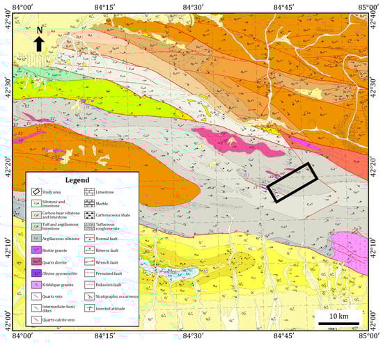
Figure 1.
Location map and geological background of Huola Mountain.
The tunnel passes through Huola Mountain as a whole. Huola Mountain is located in the middle of the Xinjiang Uygur Autonomous Region, at the junction of south Tianshan Mountains and the northeast edge of Tarim Basin, close to Bosten Lake, the largest inland freshwater lake in China. Huola Mountain is connected to the Great Youerdus Basin in the north, Kuqa Fold Belt in the west, and Yanqi Basin in the northeast. Korla, the second largest city in Xinjiang, is located in front of the southeast mountain. The mountain is NW–SE trending, with a total length of about 245 km and a north–south width of about 30–60 km. It gradually narrows from west to east, similar to a wedge-shaped distribution. The terrain is high in the west and low in the east. Elevation gradually decreases from nearly 4200 m in the northwest to about 1100 m in the southeast [].
The regional strata mainly consist of Paleoproterozoic (Pt1Ar), Devonian (D), Carboniferous (C), Neogene (N), and Quaternary (Q) materialsin the Huola Mountain Tunnel area. According to previous regional geological data, Huola Mountain Tunnel is crosscut by five faults (numbered F1 to F5, respectively) []. The four E–W-trending faults are nearly parallel. The F4 and F5 faults are crosscut by the F3 NW–SE trending strike-slip fault with about 300 m strike-slip distance. The F1 fault mainly occurs in the contact zone between the Carboniferous and the Quaternary strata. The F2 fault is present within the Carboniferous strata. The F3–F5 faults are present in the contact zone between the Carboniferous, Devonian, and Precambrian strata. The core Early Carboniferous strata is a uniform shallow marine carbonate sedimentary formation [].
The tunnel site is predominantly in a medium–high mountain area. The tunnel entrance is located at K44+970 along the line. On the southern slope of the mountain, the terrain gradient is 40°–55° and the terrain is steep. The tunnel entrance trend intersects with the slope nearly vertically. The tunnel exit is located at the line K53+490. On the north slope of the mountain, the terrain gradient is about 35°, terrain is steep, and slope vegetation is not developed. The tunnel exit trend intersects with the slope nearly vertically. The thickness of the overburden in the tunnel site is unevenly distributed. The overburden at the tunnel entrance and exit is thin. The bedrock in the tunnel is exposed. The lithology of the bedrock in the tunnel site is mostly calcareous sandstone and a small amount of limestone [,]. The entrance of the tunnel site is located in Keyilike Ditch, Cedaya Township, Luntai; its exit is located in the Malgaiti Ditch, Bayanbulak, Hejing County. The mountains on both sides of the entrance and exit are steep, and, thus, the area has no conditions of traffic. Therefore, we used ground–airborne and airborne electromagnetic methods to examine the area.
3. Tunnel Detection Method
The primary purpose of this survey was to determine the apparent resistivity profile and geological mapping of the Huola Mountain Tunnel site area, and infer the major stratigraphic boundaries, fault fracture zones, rock fragmentation, weakness, karst development, and water content, so as to provide some geotechnical risk references for the safe construction of tunnels. We conducted aerial and airborne and ground–airborne electromagnetic surveys in the Huola Mountain Tunnel section. The helicopter-borne time-domain electromagnetic method can obtain high-resolution apparent resistivity imaging results of shallow sections (0–300 m), while the apparent resistivity profiles of deep sections (200–2200 m) can be obtained by the ground–airborne frequency-domain electromagnetic method [].
3.1. Layout of the Survey Lines
We set up 15 survey lines (Figure 2) to ensure the integrity of the detection data, adequate resolution, and adequate signal-to-noise ratio in the measurement area, and to guarantee that the design is convenient, economic, and reasonable for actual flight. In total, 11 parallel survey lines, numbered L01–L11 from north to south, were set along the tunnel direction on both sides of the tunnel central line L06. In actual flight, L06 was set as a repeated flight line. Each measuring line was 9.9 km long, extending 700 m at the entrance and exit of the tunnel. Among the 11 survey lines, the interval of adjacent lines was set to 30 m for L4–L8, and 50 m for L1–L4 and L8–L11. Simultaneously, to identify the abnormal area better, four vertical survey lines were arranged in the location above the tunnel where the terrain fluctuated violently, the surface water system was developed, and tunnel burial depth was large. The corresponding number from the exit to the entrance was T1–T4.
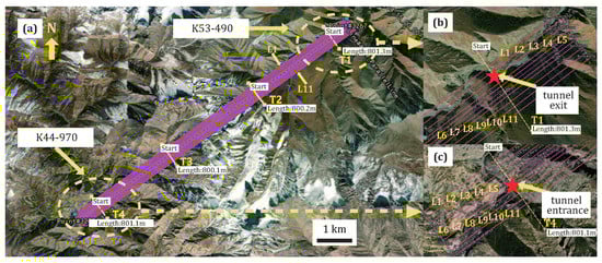
Figure 2.
Flight line map over a satellite image. (a) General survey line layout. (b) Tunnel exit survey line layout. (c) Tunnel entrance survey line layout.
3.2. HTEM System and Data Acquisition
The HTEM system is primarily composed of internal instruments and external pod devices in the engine room. The basic composition of the equipment is shown in Figure 3. The instruments in the aircraft cabin include a power supply, a transmitter, a receiver, and auxiliary instruments. The pod device carries the transmitting coil, compensating coil, and receiving sensor. It is attached to the bottom of the helicopter by a loose rope. The instrument in the cabin and the one on the pod device transmit signals through a long transmission cable tied to a sling rope. In the experiment, the diameter of the pod was 18.1 m. The emission current was a bipolar triangular wave with a pulse width of 2.4 ms and a peak current of 470 A. The turn-off time of the triangular wave was 1.16 ms, and current linearity was good during the turn-off period. The transmitting magnetic moment was 47.8 × 10⁴ A2. The sampling frequency of the receiving system was 192 kHz.
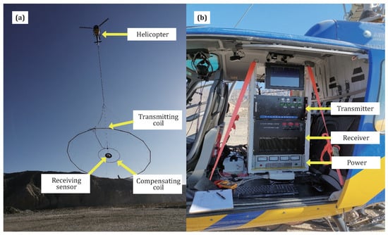
Figure 3.
HTEM system on survey. (a) External system of helicopter cabin. (b) Internal system of helicopter cabin.
3.3. GAFEM System and Data Acquisition
The basic composition of the GAFEM system is shown in Figure 4. The system is composed of three parts: an airborne magnetic field recording system, a ground high-power transmission system, and a ground reference base station. The airborne magnetic field recording system is composed of a cabin receiver, a radar altimeter, a global positioning system, and other auxiliary equipment, such as a z-component hollow magnetic induction sensor outside the cabin and an x–y-component magnetic induction sensor that is used to collect the magnetic field information of the system under the 3D coordinates of the survey area. The ground high-power transmission system includes three-phase alternating current generated by the generator. The high-power multifrequency pseudorandom wave transmitter forms an electrical source transmission system through two electrodes and the Earth. The ground reference station is composed of a receiver and a three-component magnetic induction sensor that is responsible for recording the changes in the magnetic field of the surrounding space. In contrast with the HTEM system, the ground artificial excitation field source is deployed 3.8 km southwest of the survey line entrance for the ground–airborne GAFEM detection method.
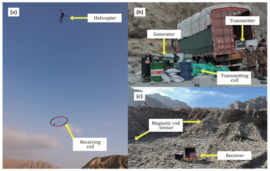
Figure 4.
GAFEM system on survey. (a) Airborne magnetic recording system. (b) Ground high-power transmitting system. (c) Ground electromagnetic reference station.
The ground high-power transmission system takes the Earth as the load and uses a superpowered electrical source with an electrical dipole moment of 3 km for detection. The transmitting current is a bipolar pseudorandom wave with a fundamental frequency of 16 Hz, the peak current is 18 A, the grounding resistance is 68 Ω, and the working voltage is 1200 V. One flight can simultaneously acquire the signals of 27 frequencies. The sampling frequency of the airborne magnetic field recording system is 192 kHz, and the diameter of the receiving coil is 8 m. The data collected by the receiving system are electrical signals, and the magnetic field is obtained through data preprocessing.
4. Data Processing and Imaging Results
4.1. Data Processing of the HTEM System
First, the background field data were interpolated two times (before and after the flight of the survey line) to obtain the background field correction value of the system during the flight of the survey line, and the background field correction of the HTEM data was completed. Second, the clipping and wavelet filtering methods were used to eliminate natural background electricity noise and motion noise generated by helicopter and coil movement, respectively. We used the attitude information measured by the navigator to calibrate the data [,]. Finally, the data that were collected within 1 s were stacked to extract traces with an equal logarithmic interval (total of 21 gates). The data of L5 and L7 are shown in Figure 5.
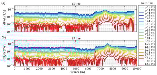
Figure 5.
Field measured data by the HTEM system. (a) L5 line. (b) L7 line.
4.2. Data Processing of the GAFEM System
For the navigation data collected by the GAFEM system, we first converted the coordinate data of the navigation system into geodetic coordinates. A fast Fourier transform (FFT) was performed on the transmission current data to obtain the effective value of the current that corresponded to each transmission frequency. Second, for the data obtained from the receiving coil sensor, the wavelet and full-period superposition methods were used to correct the motion baseline and suppress random noise, respectively. Then, FFT was used to obtain the effective signal value of each frequency. Finally, we determined the magnetic field amplitude through magnetic field calibration and current normalization. The magnetic field data of measuring lines L3 and L4 are presented in Figure 6.
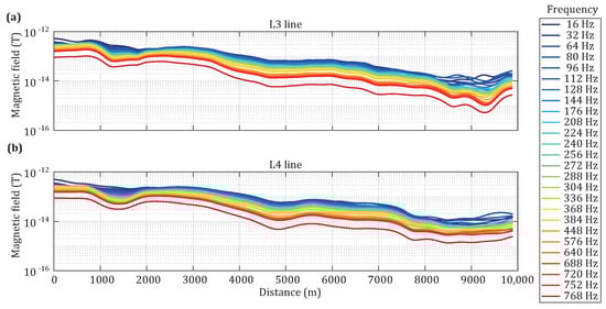
Figure 6.
Field measured data of the GAFEM system. (a) L3 line. (b) L4 line.
4.3. Apparent Resistivity Imaging Results
For each measuring line, we calculated the apparent resistivity and apparent depth of HTEM using the measured electromagnetic induction data (some lines are shown in Figure 5) and obtained the imaging results within the range of 0–300 m []. Simultaneously, we calculated the apparent resistivity and apparent depth of GAFEM using the measured electromagnetic field data (some lines are shown in Figure 6) and obtained resistivity results of 200–2200 m [,]. For the steep terrain of Mount Hora, we used known terrain parameters, flight height, coil attitude angle, etc., when modeling HTEM and GAFDEM. Therefore, the apparent resistivity imaging results calculated using electromagnetic response data only include the influence of geological structure anomalies. Finally, we used the Kriging interpolation method to fuse the apparent resistivity results obtained by HTEM and GAFEM, and obtained the apparent resistivity imaging results in the entire survey area. The apparent resistivity imaging results of survey lines L2, L4, L6, and L8 are presented in Figure 7. The 3D slices T1–T4 of the horizontal apparent resistivity are shown in Figure 8, where the L serial number represents the survey line and the T serial number represents the horizontal resistivity slice.
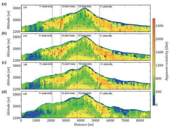
Figure 7.
Apparent resistivity result of the survey line. (a) L2 line. (b) L4 line. (c) L6 line. (d) L8 line.
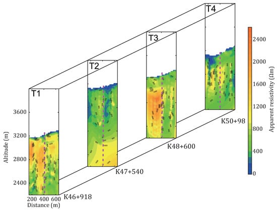
Figure 8.
A 3D slice of the apparent resistivity.
Figure 7 and Figure 8 illustrate that the apparent resistivity of K46+040–K51+000 is high, with the lowest resistivity of about 400 Ωm and the highest resistivity of about 1600 Ωm. Resistivity exhibits evident stratification. Yellow indicates relatively high resistance from top to bottom, while green indicates relatively low resistance. At K50+640–K51+200, the tunnel body’s crossing resistivity is high. However, an evident low-resistance anomaly of equivalent coil closure is notable directly above the tunnel’s main body in this area. The two low-resistance values are significantly characterized by downward extension, and their center positions have low resistance, with a resistivity of about 200 Ωm. At K52+080–K53+490, the apparent resistivity distribution map shows that the shallow low resistivity is characterized by a downward extension. Combined with the aerial images, the low-lying areas are characterized by a downward extension of low-resistivity anomalies. At K53+120–K53+300 and K53+400–K53+490, the tunnel body passes through the low-resistivity abnormal area.
In accordance with the overall apparent resistivity imaging results presented in Figure 7 and Figure 8, we obtained the resistivity distribution of the tunnel body’s survey line, as shown in Figure 9. The resistivity distribution map of the tunnel trunk’s survey line consists of three parts: the entrance turning, the tunnel trunk, and the exit turning. The turning point at the entrance (K44+970-K45+120, total of 150 m) was obtained by processing the data of the survey lines adjacent to L6. The main body of the tunnel was obtained from processing the data of the L6 survey line. The turning point at the exit (K52+970-K53+470, total of 500 m) was obtained by processing the survey lines adjacent to L6.
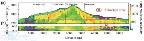
Figure 9.
Apparent resistivity results: (a) apparent resistivity slices of the tunnel; (b) apparent resistivity map at the depth of the tunnel.
Figure 9b shows a tile map of apparent resistivity at the depth wherein the tunnel body is located. The colors ranging from purple to red represent the resistivity value from low to high. Analyzing the image can obtain information, such as apparent resistivity morphology and characteristics. As shown in the image, the background value of resistivity of the rock mass in this section is above 80 Ωm. The shallow part of the mountain surface generally exhibits low resistivity. Another two low-resistivity anomalies are D1 and D2, respectively, with resistivity values less than 300 Ωm, which can be interpreted by highly jointed and saturated sandstone deposits.
The lowest resistivity of the D1 low-resistivity anomaly is about 158 Ωm, and the highest is about 250 Ωm. It is an anomaly of the vertical long strip trap, and resistivity is low at the center. The outcrop sandstone stratum experienced strong weathering. The rocks developed large amounts of fractures and joints, which resulted in large quantities of water occurring in the rock-breaking cracks. Based on the above field characteristics, we speculate that the D1 low-resistivity anomaly is caused by fragmented rocks with plenty of water filling them. The D1 low-resistivity anomaly is close to the F2 fault shown in Figure 1. Therefore, the broken rocks may be affected by the fault, proving the accuracy of the resistivity imaging results. The tunnel body passes through this anomaly, and, thus, considerable attention should be given to this anomaly.
The lowest value of the D2 low-resistivity anomaly is about 125 Ωm, while the highest value is about 200 Ωm. In accordance with the aerial photography data, the area is low-lying, with two water-rich ditches above the tunnel body. The rocks at K51+000–K52+080 experienced strong erosion by mountain top drainage for a long time, which resulted in a lot of water in the shallow part of the area. The outcrop sandstone stratum experienced strong weathering, which resulted in the breaking rocks developed plenty of cracks. Due to the relatively low altitude, a great deal of water collects in the D2 anomaly area. Therefore, the D2 anomaly was caused by fragmented rocks and water. The D2 low-resistivity anomaly is close to the F3 fault in Figure 1. Therefore, the broken rocks may be affected by the fault, proving the accuracy of the resistivity imaging results. The tunnel body passes through or is directly above the tunnel body, and considerable attention should be given to this anomaly.
In order to meet the needs of disaster prevention and rescue in the tunnel, a parallel pilot tunnel is set up 35 m to the right side of the tunnel. The apparent resistivity results of the parallel pilot tunnel are shown in Figure 10. The overall apparent resistivity characteristics of the parallel pilot tunnel and the tunnel body are basically consistent, and the apparent resistivity profile shows that the background resistivity value of the rock in this section is above 80 Ωm. According to the shape and characteristics of apparent resistivity, two low-resistivity anomalies are delineated as D1 and D2, and resistivity is less than 300 Ωm.
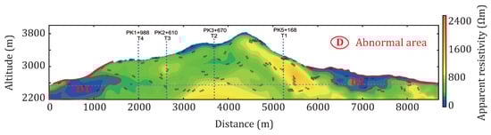
Figure 10.
Apparent resistivity imaging result of the parallel pilot tunnel, which is located 35 m southeast of the tunnel.
The apparent resistivity between D1 and D2 low-resistivity anomalies is relatively high, with a minimum resistivity of about 400 Ωm and a maximum resistivity of about 1600 Ωm. It is similar to the resistivity distribution characteristics of the tunnel body, with apparent sandstone resistivity layering. In the field observation, the sandstone stratum shows the characteristic of stratification with different grain size. Furthermore, the study area experienced a strong fold deformation event, which resulted in different-grain sandstones showing different features of apparent resistivity. Therefore, we speculate the stratification characteristics of apparent resistivity caused by the rocks with different degrees of crushing strength. Similarly, in accordance with the resistivity profile of this section and the resistivity distribution of the T2 line profile, rocks in the middle of this section may have developed plenty of joints and cracks. Simultaneously, due to the deep burial depth in this section, local small-scale faults and folds cannot be precluded. Therefore, attention should be given to the area of relatively low apparent resistivity, and protection work should be implemented well.
5. Conclusions
To determine the water content in the Huola Mountain Tunnel site and ensure construction safety, we conducted HTEM and GAFEM electromagnetic surveys in the Huola Mountain Tunnel site where ground personnel experience difficult access and the tunnel is deeply buried. In this HTEM and GAFEM geophysical exploration, 15 survey lines were surveyed, and we conducted apparent resistivity imaging for each line. The apparent resistivity results of each profile obtained by the fusion of two kinds of electromagnetic detection data were consistent, proving the reliability of the results. We determined that the overall distribution of apparent resistance was basically consistent with the site’s landform, hydrogeology, and tectonic geology. In accordance with relevant geological data, topographic conditions in the survey area, and aerial image data, we speculated that the surrounding rock in some deep sections of the tunnel is complete. However, there are two low-resistance abnormal areas at the entrance and exit of the tunnel, which are consistent with the positions of two known faults. It is inferred that the shallow surrounding rock in the tunnel site was seriously weathered and rock fissures had developed, especially in low-lying areas, where the rocks have been eroded by the drainage of the mountaintop for a long time. When construction reaches the area with large water content, roof fall, block fall, and water or mud gushing may occur. Making geological predictions and implementing drainage and other relevant measures in advance, such as tunnel seismic prediction, ground penetrating radar, and bore-tunneling electrical monitoring, are recommended to ensure construction safety.
Author Contributions
Conceptualization, T.Z. and Y.W.; data curation, H.Z., S.W. and G.L.; formal analysis, C.Z. and D.L.; funding acquisition, Y.W.; investigation, H.Z., S.W. and F.Z.; methodology, H.Z., S.W. and C.J.; resources, G.L. and F.Z.; validation, H.L.; writing—original draft preparation, T.Z., C.Z., D.L. and C.J.; writing—review and editing, H.L. All authors have read and agreed to the published version of the manuscript.
Funding
This research was funded by the National Natural Science Foundation of China, grant number 42004059, and National Key R&D Program of China, grant number 2017YFC0601802.
Institutional Review Board Statement
Not applicable.
Informed Consent Statement
Not applicable.
Data Availability Statement
The data that support the findings of this study are available on request from the corresponding author.
Conflicts of Interest
The authors declare no conflict of interest. The funders had no role in the design of the study; in the collection, analyses, or interpretation of data; in the writing of the manuscript; or in the decision to publish the results.
References
- Fountain, D. Airborne electromagnetic systems-50 years of development. Explor. Geophys. 1998, 29, 1–11. [Google Scholar] [CrossRef]
- Kaiguang, Z.; Yidi, P.; Xiaoshuang, Z.; Zeli, Q.; Cong, P. Time-frequency characteristic analysis of electromagnetic detection of motion noise. J. Jilin Univ. (Eng. Technol. Ed.) 2019, 49, 319–324. [Google Scholar]
- Gao, L.; Yu, S.; Zhou, H.; Liu, C.; Chen, N.; Huang, Y. Depth-focused waveform based on SHEPWM method for ground-airborne frequency-domain electromagnetic survey. IEEE J. Sel. Top. Appl. Earth Obs. Remote Sens. 2019, 12, 1981–1990. [Google Scholar] [CrossRef]
- Smith, R.S.; Annan, A.P.; McGowan, P.D. A comparison of data from airborne, semi-airborne, and ground electromagnetic systems. Geophysics 2001, 66, 1379–1385. [Google Scholar] [CrossRef]
- Liang, S.; Zhang, L.; Cao, X.; Liu, Q. Research progress of the time-domain airborne electromagnetic method. Geol. Explor. 2014, 50, 0735–0740. [Google Scholar]
- Lin, J.; Kang, L.; Liu, C.; Ren, T.; Zhou, H.; Yao, Y.; Yu, S.; Liu, T.; Liu, P.; Zhang, M. The frequency-domain airborne electromagnetic method with a grounded electrical source. Geophysics 2019, 84, E269–E280. [Google Scholar] [CrossRef]
- Di, Q.; Xue, G.; Yin, C.; Li, X. New methods of controlled-source electromagnetic detection in China. Sci. China Earth Sci. 2020, 63, 1268–1277. [Google Scholar] [CrossRef]
- Dazhi, T.; Liu, Y.; Wang, Y.; Yuewen, Y.; Weilin, Z.; Jinfu, L.; Na, A. A Height-Correction Method for Airborne Transient Electromagnetic Measurement of the Triangle-Wave Field Source. Geol. Explor. 2022, 400, 129–137. [Google Scholar]
- Boyko, W.; Paterson, N.; Kwan, K. AeroTEM characteristics and field results. Lead. Edge 2001, 20, 1130–1138. [Google Scholar] [CrossRef]
- Smith, R.S.; Hodges, G.; Lemieux, J. Case histories illustrating the characteristics of the HeliGEOTEM system. Explor. Geophys. 2009, 40, 246–256. [Google Scholar] [CrossRef]
- Goebel, M.; Knight, R.; Halkjær, M. Mapping saltwater intrusion with an airborne electromagnetic method in the offshore coastal environment, Monterey Bay, California. J. Hydrol. Reg. Stud. 2019, 23, 100602. [Google Scholar] [CrossRef]
- Shengbao, Y.; Changyu, S.; Jian, J.; Jun, L.; Xuefeng, C.; Jean, L.; Greg, H. Research on CHTEM-I Helicopter Time-Domain Aeronautical Electromagnetic Launch System. J. Cent. South Univ. 2019, 48, 1552–1559. [Google Scholar]
- Huaiyuan, L.; Jingxun, Z.; Minzhong, J.; Yan, L.; Donghua, S. The application effect analysis of the VTEMplus system. Geophys. Geoochem. Explor. 2016, 40, 360–364. [Google Scholar]
- Zhou, H.; Lin, J.; Liu, C.; Kang, L.; Li, G.; Zeng, X. Interaction between two adjacent grounded sources in frequency domain semi-airborne electromagnetic survey. Rev. Sci. Instrum. 2016, 87, 034503. [Google Scholar] [CrossRef] [PubMed]
- Sørense, K.; Auken, E. SkyTEM? A new high-resolution helicopter transient electromagnetic system. Explor. Geophys. 2004, 35, 194–202. [Google Scholar] [CrossRef]
- Ito, H.; Kaieda, H.; Mogi, T.; Jomori, A.; Yuuki, Y. Grounded electrical-source airborne transient electromagnetics (GREATEM) survey of Aso Volcano, Japan. Explor. Geophys. 2014, 45, 43–48. [Google Scholar] [CrossRef]
- Auken, E.; Christiansen, A.V.; Westergaard, J.H.; Kirkegaard, C.; Foged, N.; Viezzoli, A. An integrated processing scheme for high-resolution airborne electromagnetic surveys, the SkyTEM system. Explor. Geophys. 2009, 40, 184–192. [Google Scholar] [CrossRef]
- Høyer, A.S.; Lykke-Andersen, H.; Jørgensen, F.; Auken, E. Combined interpretation of SkyTEM and high-resolution seismic data. Phys. Chem. Earth, Parts A/B/C 2011, 36, 1386–1397. [Google Scholar] [CrossRef]
- Ji, Y.; Wang, Y.; Xu, J.; Zhou, F.; Li, S.; Zhao, Y.; Lin, J. Development and application of the grounded long wire source airborne electromagnetic exploration system based on an unmanned airship. Chin. J. Geophys. 2013, 56, 3640–3650. [Google Scholar]
- Cong, Y.; Lifeng, M.; Xinxin, M.; Cheng, W.; Ming, G. Study on the Semi-Aerospace Transient Electromagnetic Adaptive Regularization-Damped Least Squares Algorithm. Geol. Explor. 2020, 56, 137–146. [Google Scholar]
- Zhang, M.; Liu, C.; Farquharson, C.G. 2.5-D forward modeling of the frequency-domain ground-airborne electromagnetic response in areas with topographic relief. Chin. J. Geophys. 2021, 64, 327–342. [Google Scholar]
- Bin, C.; Lifeng, M.; Guangding, L. Estimation of detection depth of CHTEM-I system with diffusion electric field method. Acta Geophys. Sin. 2014, 57, 303–309. [Google Scholar]
- Zhu, K.G.; Lin, J.; Han, Y.H.; Li, N. Research on conductivity depth imaging of time domain helicopter-borne electromagnetic data based on neural network. Chin. J. Geophys. 2010, 53, 743–750. [Google Scholar]
- Zhou, H.; Yao, Y.; Liu, C.; Lin, J.; Kang, L.; Li, G.; Zeng, X. Feasibility of signal enhancement with multiple grounded-wire sources for a frequency-domain electromagnetic survey. Geophys. Prospect. 2018, 66, 818–832. [Google Scholar] [CrossRef]
- Zhang, Y.Y.; Li, X.; Yao, W.H.; Zhi, Q.Q.; Li, J. Multi-component full field apparent resistivity definition of multi-source ground-airborne transient electromagnetic method with galvanic sources. Chin. J. Geophys. 2015, 58, 2745–2758. [Google Scholar]
- Yuan, Y.; Jianbo, C.; Shuai, L.; Heping, S.; Jiangli, X. Late-Quaternary activity characteristics of Akeaiken segment of Beiluntai fault belt at south of Tianshan, in Xinjiang. Quat. Sci. 2017, 37, 645–653. [Google Scholar]
- Yang, X.; Li, A.; Hunag, W. Uplift differential of active fold zones during the late Quaternary, northern piedmonts of the Tianshan Mountains, China. Sci. China Earth Sci. 2013, 56, 794–805. [Google Scholar] [CrossRef]
- Huang, W.; Yang, X.; Jobe, J.A.T.; Li, S.; Yang, H.; Zhang, L. Alluvial plains formation in response to 100-ka glacial–interglacial cycles since the Middle Pleistocene in the southern Tian Shan, NW China. Geomorphology 2019, 341, 86–101. [Google Scholar] [CrossRef]
- Lin, J.; Xue, G.; Li, X. Technological innovation of semi-airborne electromagnetic detection method. Chin. J. Geophys. 2021, 64, 2995–3004. [Google Scholar]
- Becken, M.; Nittinger, C.G.; Smirnova, M.; Steuer, A.; Martin, T.; Petersen, H.; Meyer, U.; Mörbe, W.; Yogeshwar, P.; Tezkan, B.; et al. DESMEX: A novel system development for semi-airborne electromagnetic exploration. Geophysics 2020, 85, E253–E267. [Google Scholar] [CrossRef]
- Ito, H.; Mogi, T.; Jomori, A.; Yuuki, Y.; Kiho, K.; Kaieda, H.; Suzuki, K.; Tsukuda, K.; Allah, S.A. Further investigations of underground resistivity structures in coastal areas using grounded-source airborne electromagnetics. Earth, Planets Space 2011, 63, e9–e12. [Google Scholar] [CrossRef]
Disclaimer/Publisher’s Note: The statements, opinions and data contained in all publications are solely those of the individual author(s) and contributor(s) and not of MDPI and/or the editor(s). MDPI and/or the editor(s) disclaim responsibility for any injury to people or property resulting from any ideas, methods, instructions or products referred to in the content. |
© 2023 by the authors. Licensee MDPI, Basel, Switzerland. This article is an open access article distributed under the terms and conditions of the Creative Commons Attribution (CC BY) license (https://creativecommons.org/licenses/by/4.0/).