Abstract
Smart surfaces are becoming more and more popular in the field of intralogistics, as they combine great flexibility with easy reprogrammability. Pursuing this trend, the following article proposes a modular surface to perform handling tasks, such as sorting, stopping, or slowing down material flows. Differently from the current technology, the surface used is under-actuated, thus, it exploits the speed, already possessed by the object, or the gravity to perform, with a simplified hardware, for the aforementioned tasks. In practice, these handling actions are completed using an array of rotors, of which only the direction of the rotation axis is controlled. Moreover, the axis can only assume certain discrete orientations in the plane, further simplifying the design. Thus, what is created is a controllable and under-actuated friction field, which, in contrast with similar existing systems, does not require active driving forces to manipulate the material flow. In the article, the analytic model of the surface is described, and a software simulation environment is introduced to demonstrate its functioning. In addition, examples of sorting, slowing down, and stopping operations and a validation of the simulation itself are presented.
1. Introduction
The material transport inside factories and warehouses is a very studied topic. However, companies are always searching for new, cheaper solutions while keeping an eye on efficiency and flexibility [1,2,3,4]. Starting with the most basic conveyors, many alternative systems [5,6,7,8,9,10,11,12] have been developed in order to move, sort, orient, and handle the material flow. More recently, the focus of investigation has shifted towards modular devices and surfaces that allow high handling capability, adaptability, and reconfigurability [3,4,13]. This happens because the market increasingly demands a flexible industry, and this is reflected in all production levels, even the internal transportation. These devices are often called smart surfaces because they are controllable and reprogrammable with computers. Thanks to these characteristics, these new systems permit achieving their goals without structural changes [4,13]. In addition, the new devices are capable of identifying a part with sensors and acting in diverse ways, according to their programming. As a result, supervision by an operator is no longer required for the decision process and the system becomes autonomous, promising to reduce errors and costs [14].
The most relevant solutions among the smart surfaces, according to the current state of the art and classified by the operating principle, are: micro electro-mechanical systems, vibrating surfaces, ciliary motion, variable morphology surfaces, pneumatic surfaces, surfaces with rotors, and mobile platforms. Micro electro-mechanical systems (MEMS) [6,15,16] are an array of microscopic cantilevers or tilting planes, actuated electrically, that generate forces to transport the object in contact. The second category of the list are vibrating surfaces. These consist of vibrating plates on which a sequence of supply frequencies is applied to generate a two-dimensional force field for the handling tasks [5,17]. In [12,18,19,20], ciliary motion is proposed to move and manipulate objects, taking advantage of an array of controllable cilia for contact conveyance. Another class are variable morphology surfaces [9,21,22,23]. For these devices, gravity together with inclined planes and vertical actuators at different altitudes are used to create a preferential path for the movement and rotation of an object. Additionally, pneumatic surfaces [7,24,25,26,27,28,29,30] were introduced to handle materials without direct contact. The working principle for the latter is to have modules with nozzles to move parts by directing the air flow below them. On the other hand, surfaces with rotors take advantage of contact forces made by actively driven wheels to manipulate the material flow [3,11,13,14,31,32,33,34,35]. Finally, mobile platforms [8,36,37,38,39] consist of mobile pallets, not connected to fixed axes and free to move on a plane, transporting objects on top. Despite the categorization, not all of these are practically used for macroscopic intralogistics purposes (object size and displacement > cm). In fact, as summarized in Figure 1, some of them, such as MEMS, together with some mobile platforms [8,37,38,39] and ciliary devices [12,18,19], are more suitable for microscopic transport (object size and displacement < mm). In contrast, pneumatic systems, vibrating surfaces, surfaces with rotors, variable morphology surfaces, some mobile platforms [36], and even tilted brushes (Cilia) [20] can be used to move macroscopic and mesoscopic (object size and displacement > mm, <cm) objects.
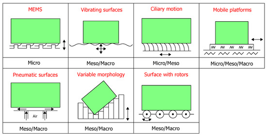
Figure 1.
Smart surfaces classification and field of application.
Referring to the previous classification, the system proposed in this paper can be included in the surfaces with rotors category. The literature review conducted on this category identified two main types of modular smart surfaces: systems where each module has only one degree of freedom [3,11,13,35] and systems where each module has two [14,34]. The former, which are the most recent in the literature, exploit multiple omnidirectional and motorized wheels called “omniwheels” positioned in the module with their axes fixed. The layout and number of wheels is not the same in every study, however; as a reference, three or more wheels are usually employed and their spinning axes are positioned out of alignment to create controllable forces in both directions of the plane. As first example of modules with more than three wheels, study [13] alternates units with seven wheels—one large in the center and six small on the sides, to units with five—two large on the sides and three small in the center. For both layouts, the axes of the large wheels are perpendicular to the axes of the small ones to ensure driving forces in the plane. In contrast, in [3,11,35], each module of the device studied, called “Celluveyor”, contains three omnidirectional wheels with axes arranged at 120° to one another. Each wheel can rotate at different speeds to control the magnitude of the force exchanged with the transported object, and all three forces together are used to handle the body motion. On the other hand, the second group of systems, i.e., those with modules with two degrees of freedom, consist of units composed of one or more motorized and swiveling wheels. In this case, therefore, as presented in [14,34], the basic element of the module is a simple wheel driven by a motor mounted on its axis of rotation. This wheel, however, unlike the one degree of freedom systems, is also mounted on a vertical axis, which is itself motorized and therefore swiveling. Summarizing, these devices just described are fully implemented and contain several motors per module, specifically, three or more for the first class and at least two for the second. They can actively drive, sort, and manipulate the material flow, creating a totally actuated surface with significant handling skills. However, the use of several motors and their control necessarily involves a greater effort in the management of the system, as well as increasing costs and complexity. According to the current state of the art, a simpler under-actuated device without motors is missing for the same intralogistic tasks. For that reason, seeking cost reduction and simplification of both control and design, without losing the flexibility of this class of systems, in this paper the authors propose an under-actuated surface composed of modules. Unlike existing concepts, each module contains an idle rotor instead of a motorized wheel. The axis of rotation of the mentioned rotor is not driven continuously by a motor but can be oriented in a limited number of directions in the plane of the surface, creating a directionable friction force for object handling. In order to compensate for the under-actuation, the material is moved by exploiting gravity or an initial velocity of the object provided by another system (e.g., a previous conveyor belt). Therefore, compared to the existing systems [3,11,13,14,31,32,33,34,35], the novelty that distinguishes this active surface from the literature technology lies in its simplicity. In fact, the two main characteristics of the system proposed by the authors, compared to those in the same category, are the under-actuation and the limited directions of the rotor axis, both of which are reductions to a minimal form of concept technology, but which save components and make the most of sources already present in the application environment, such as gravity and the speed of the objects in the transport line. Against potential assumptions of performance losses, the authors proved through simulations that the same goals and efficiency [3,4,35] of sorting and handling can be achieved with a minimal design architecture, consisting of few components, while decreasing costs and saving energy.
The focus of this article lies on the study of the surface, the description of the working principle, and its simulation with the purpose of providing an initial proof of concept for possible applications and future developments. Furthermore, the simulation environment allowed numerical results to be obtained for typical intralogistics tasks, giving the opportunity for an initial comparison with the corresponding current technology. The simulations presented in this article are carried out with a customized code developed by the authors using the software MATLAB (Version R2022a). In addition, a validation of the simulation results was obtained with the well-known program for multi-body dynamic simulations Hexagon D&E Adams MSC (Version 2022.1). The authors decided to develop their own simulation environment because of its significant lower computing time. Thus, their software is eligible to control the actual physical system in real time in the future.
The remainder of this paper is organized as follows: Section 2 describes the concept of the surface. Section 3 explains the analytic model used to describe the working principle. Section 4 describes the simulations of the system for different tasks. Finally, Section 5 reports the results, Section 6 consists in the validation of the latter, and Section 7 describes the conclusions.
2. Concept Description
This section provides a qualitative description of the functioning of the surface and the modules of which it is composed. The operating principle of the surface is based on an array of modules with an idle rolling element and an orientable axis of rotation. These axes are used to generate directionable friction forces on the body in contact with the surface. The origin of the friction forces lies in the very working principle of a rotor. In fact, these are constructed and used (e.g., conveyor rollers) to facilitate motion in one direction (perpendicular to their axis of rotation). This leads to a difference in the friction forces exchanged with an overlying object.
In practice, there will be a smaller component, perpendicular to the axis, caused mainly by rotational friction, and a larger one, parallel to the axis, due to linear friction ( and , respectively, in Figure 2c). Therefore, the main friction component will be predominantly along the axis, so by orienting the latter, the main force will also be directed. The choices of the axis directions are limited to a fixed number. For example, the simplest configuration is with two orientations (, ), whereas more complex designs are with four (0, , 45, 90) (Figure 2b) or more. In Figure 2b, the four orientations are shown, with the rotors displayed like cylinders (the projection is a rectangle) and the axes like dashed lines. For applications such as slowing or stopping the material flow, two orientations may be enough, whereas for sorting, four orientations should be taken into account. Therefore, modules with four directions will be considered in the following pages. For its intended applications, the module must be used together with others to create the surface (Figure 2a), so the sum of the forces exerted by every unit will control the objects for sorting and feeding purposes. In Figure 2a, the surface setup is summarized, showing the grid of modules with the object on top, and the arrows inside each cell represent directions of motion promoted by them. As noted in the introduction section, the system is under-actuated, so the surface can only slow down the object while it completes its task of sorting or feeding. If, for example, a body is simply placed on the surface without external actuation, it will not move. To overcome this situation, the surface plane can be tilted to use the gravity effect as the missing actuation, or an initial velocity can be given to the part before crossing the surface. Depending on the application and the task of the system, one solution may be preferred over the other, or a combination of both may be chosen. For instance, if the extension of the surface is big, because the objective is to orient a body, the tilted solution could be better, whereas, if the goal is to sort parts in a conveying line, the initial velocity of the object, given by the conveyors before the sorting area, is enough.
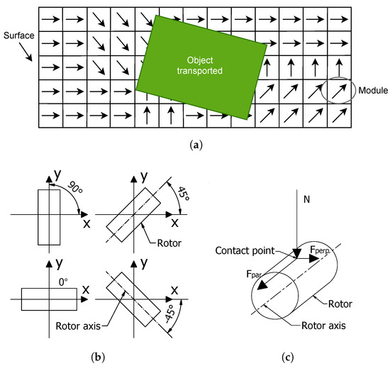
Figure 2.
Illustration of: (a) the modular active surface, (b) the four possible orientations of the rotors, and (c) the three contact forces between the object and the rotor.
In addition, similar to other active surfaces that use rotors for intralogistic purposes, the application is limited to parts with at least one planar surface, in order to have simultaneous contact with three or more rotors. Another limit will be the maximum load per module, but this is related to the resistance of the device, which is not studied in this article. However, the study conducted is done considering the dimensions of the modules and their resistance comparable with the similar actuated existing systems. To provide a reference, the base of a transported object has the minimum dimensions of cm cm], and the weight bearable by a single module is 20 kg.
3. Analytical Model
Continuing with the description of the functioning of the surface, this section reports the hypothesis, the forces involved to move the objects, and the model applied to determine these, respectively, in the subsections Assumptions, Friction Forces Model, and Equilibrium Equations. As stated in Section 2, the working principle of the module is based on the contact forces exchanged between the rotor and the transported object. With this in mind, the analysis starts from the actions on a single module and then expands to the whole surface and to the equations describing the motion of an object.
Figure 3 introduces the notation used in the next pages. In particular, are the coordinates of the object’s center of mass, G, according to the reference frame , and is the projection of G on the object base along the Z axis (Figure 3a).
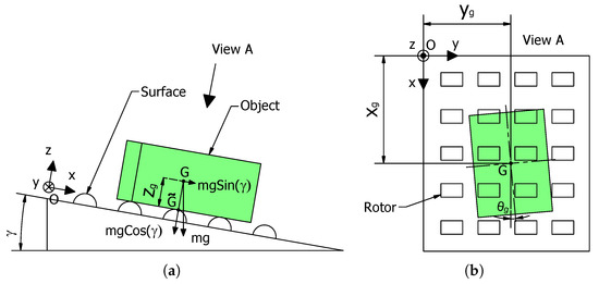
Figure 3.
Schematic illustration of the object on the surface: (a) lateral view, (b) upper view.
3.1. Assumptions
Listed here are the fundamental assumptions that allowed the definition of the analytical model describing the motion of an object on the surface.
- The first assumption states that there are only the three forces for each interaction rotor-object: two components in the plane of the device and one normal to this (Figure 2c). Considering that the contact area of the module below the object is small compared to the object itself, the previous assertion is plausible and it is translated into the possibility of neglecting the exchanged torques.
- The second assumption is about the normal component N. In fact, considering that the contact in most of the cases is on more than three rotors, the constraint is hyperstatic and the equilibrium equations of the body are not enough to determine the normal reactions. In particular, for determining the distribution of the forces , an optimization algorithm described in Equation (1) is used.where the first vector equation represents the equilibrium in the vertical direction and around the two axes of rotation in the plane, and the second vector equation states the boundary conditions. The function to be minimized is the Euclidean norm of the array. The single terms are:where n is the number of rotors under the object, m is the mass of the object, g is the gravity acceleration, and is the inclination of the surface compared to the ground (Figure 3a). In addition, and are the x and y components of the vector that connect to the ith contact point .
- The third assumption asserts that the inertia of the rotors is negligible, as they are small and made of lightweight material. Instead, the rotational friction given by the spinning of the rotor around its axis is included in the calculation of contact forces.
- The fourth assumption states that, for an object in motion on the rotors, the friction conditions at the contact points (rotors–object) are as follows: dynamic friction (sliding) in the direction of the axis of the rotors and pure rolling in the perpendicular direction. This is plausible, as the center of instantaneous rotation (CIR) of the rigid body (object) is very unlikely to be located at the center of an underlying rotor. This would guarantee a different static friction and force modeling (, ). However, with only a few discrete points as supports, it is unlikely that the CIR is located on these. In practice, for the axis direction, this assumption justifies the choice of a smooth Coulomb friction model, which is computationally stable and reliable, as the sliding condition prevails ([40]). The same model is considered for the friction force, due to the rolling, in the perpendicular direction. This value depends on the rotational friction of the rotor axis (assumption 3), so it can also be expressed using the same Coulomb formulation. More complex rotational friction models have been avoided to reduce complexity and the computational cost (for the simulation) without adding relevant contribution, as this friction component is very small and almost negligible compared to the axis direction component. In conclusion, this assumption, introducing the friction model, results in the boundary condition for the calculation of friction forces.
3.2. Friction Forces Model
In this subsection, considering the previous assumptions regarding sliding and pure rolling and taking into account that the friction forces oppose motion, the directions of the two forces (, ) and their final formulation are determined. Thanks to the third assumption, these directions are related only to the object velocity at the contact point with the rotor, ; an example is shown in Figure 4a.

Figure 4.
Schematic representations of: (a) velocities and forces exchanged in a contact point, (b) the calculation of the velocity in the contact point, (c) the resulting forces from the contacts.
In particular, the velocity can be split into a perpendicular and a parallel component (Figure 4a), and the two forces and are in the opposite directions of these velocities. In Figure 4a, three more angles are introduced: , , and (all angles are defined positive in the anti-clockwise direction from the x axis):
- is the angle between the rotor axis and the x axis;
- is the angle between the velocity of the object’s contact point and the x axis;
- is obtained by the difference between the previous two (), so it is the angle between the velocity of the body’s contact point and the rotor axis.
The velocity of the object’s contact point is determined using the formula of the kinematics of a rigid body: , where and are the linear and angular velocity of the object, and is the vector that connects to the contact point P. The velocity identification is also reported in Figure 4b, where the piece is schematized with the shape of the base, and the rotors with a grid of points. This scheme presented in Figure 4b is also useful in visualizing how the rotor–object contact points are determined. In fact, knowing the values and the mathematical formulation of the base area with respect to these, it is possible to know the set of coordinates of the points inside the base perimeter. More specifically, given a planar reference frame with coordinates , centered in () (Figure 4b) and oriented by , let Q be a set of geometrical parameters that depends on the shape of the object base (e.g., radius for a circle or base and height for a rectangle) and let . Let be a set of indexes. For every , let be functions such that is the perimeter of the object base. The area of the object base, D, is defined as . Therefore, given the coordinate pairs that define the position of the rotors in the array (which are fixed), it is verified whether or not they belong to the set, i.e., if has solution for a pair of , where is the rotation matrix of the reference frame with coordinates and centered in . Now all the elements to describe the two forces in the plane of the surface (, ) have been introduced and the result, according to Figure 4a, is summarized in Equations (2a) and (2b).
where the two friction coefficients are, respectively:
- is the friction coefficient between the object and the rotor;
- is the friction coefficient that represents the rolling resistance of the rotor.
The sgn function models the direction of the forces, according with the orientation of the object velocity in the contact point, whereas tanh and the coefficient k (selection of this parameter explained in Section 6) smooth the discontinuities ([41]). The perpendicular force would be ideally 0, however, it is generally small as inertia forces are neglected and only the rotational friction of the rotor around its axis is considered. The parallel friction force can reach significantly higher values and is opposed (in the axis direction) to the object velocity. Therefore, it is the dominant driver to manipulate the object.
3.3. Equilibrium Equations
This subsection shows how the equations of motion of the object on top of the surface are obtained from the contact force components. In practice, once these components are calculated for each contact point, they can be added together to obtain the total reactions on the part and its equilibrium equations. To achieve this, first, the friction forces in the plane at the various contact points are decomposed along the x and y directions, knowing the arrangements of the rotors ():
The signs introduced for these forces are in accordance with Figure 4a,c. The resulting equilibrium equations are summarized in Equation (4).
where , , and are, respectively, the two linear and the angular accelerations of the object; and are the coordinates of the ith point of contact; and J is the moment of inertia of the object around the axis perpendicular to the surface plane. Considering that also J can be expressed as a function of the mass, it is possible to notice that the inertia affects the system only from a structural point of view. In fact, as it is visible from the Equations (1), (2a), (2b), and (4), m can be simplified.
4. Simulations
In this section, the simulation process carried out with the analytic model implemented in MATLAB is shown. As a first step, this simulation environment permitted verifying in a general way that moving objects with the proposed theory and concept is possible. Second, it allowed several tests to be carried out in order to prove the usability of the system for some common intralogistics applications, such as sorting, orienting, stopping, and slowing down material flows.
The simulation takes advantage of an iterative loop (shown in Figure 5a) that involves the following steps: initialization, rotor identification, stopping criteria, contact forces and equilibrium computation, and two steps of integration. The initialization of the problem is made at the beginning by providing data from the object and the surface (example: object mass, base shape, initial position and velocity, friction coefficients, module pattern, inclination of the surface, rotor orientations, etc.). After that, the iterative loop can start. For each step (e.g., the sth step), the rotors below the object are identified (thus the contact points as well), knowing the position of the object from the previous iteration (th) and the disposition of the modules (as introduced in Section 3). Once the rotors below the object and their orientation are determined, the object velocity from the previous iteration (th) together with the inclination of the surface are evaluated by the stopping criteria: if “ m/s and ”, the object is stopped because of negative velocity and null inclination and the loop ends. This is true assuming, in general, that the initial conditions always provide an input towards positive x (° or ). When the stopping condition is not reached, the loop continues and the forces in the contact points can be computed (still considering the object velocity from the previous iteration (th)). With these forces, the equilibrium of the body and the accelerations are calculated according to Section 3. Finally, in order to obtain the velocity and the position, two integration steps of the acceleration vector are implemented. The derived values are the input of the next iteration (th) of the loop.
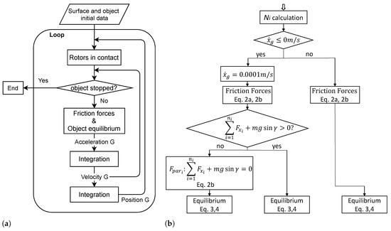
So far, the model seems to represent the operation of the surface adequately when the body velocity is greater than zero in the x direction and for the stopping condition. However, when, as an example, the object is about to start from a standstill with rotors and surface inclined, an undesirable phenomena such as reversal of motion (negative x) can occur. This happens because, in the friction assumptions, the static condition is not initially considered (Equations (2a) and (2b)). However, reverse motion is obviously not possible in reality, then, in practice, when the condition of m/s is achieved (°, otherwise the object is stopped as described before), the process needs to be adjusted. The logic instructions to solve this problem and at the same time implement the analytical model of Section 3 are summarized in the block diagram of Figure 5b, which in practice is executed inside “Friction forces & Object equilibrium” block of Figure 5a. In detail, the process works as follows: first, the terms are calculated as explained in Section 3, then, since the velocity along x is known from the previous iteration, the condition “ m/s” is verified. If it is false and “ m/s”, there is no problem of standstill or stopping and the procedure continues as described in Section 3, thus, friction forces calculation (Equations (2a) and (2b)) and equilibrium ((Equations (3a), (3b) and (4)). In contrast, if the velocity is less or equal to zero (“ m/s” is true), an initial positive speed is assigned to the object m/s, the friction model is applied, and it is verified if the gravity effect is stronger than the friction forces in the x direction (“”). At this point, if gravity wins, the object is moving according to the process defined before (Equations (3a), (3b), and (4)); in contrast, if gravity is not enough, the friction forces in the x direction will be of the same magnitude of the gravity effect (“”), and the displacement will be in the y direction (always according to Equations (3a), (3b), and (4)). To clarify the diagram of Figure 5b, the condition “” permits the calculation of the terms, while is the same as the previous case. For instance, this procedure permits us to obtain the motion of the object when it is placed without an initial velocity on the inclined surface, with the rotors oriented at 45°. In fact, with a sequence of displacement in the y and x directions, the movement is achieved.
The simulations conducted to test the surface are divided into three main categories, according to the application of the system:
- Sorting of material flows on a conveying line;
- Slowing of material flows on a conveying line;
- Stopping of material flows on a conveying line.
The first category of simulations concerns sorting. The objective of the setup and the sorting itself is to divert an object from the transport line. The layout considered for the simulation involves an array of modules, of which the subset performing the task has the rotors with the rotation axes inclined at ° (in Figure 6a inclined at °). The area outside the line, where the objects are directed, is simulated as an array of low-friction () support points, distributed as the sorting modules. In this zone, the friction is totally opposite to the velocity of the object, without considering any rotor inclination. The sorting is assumed achieved when the body moving on the line is deflected in such a way that it is only in contact with the elements outside the line.
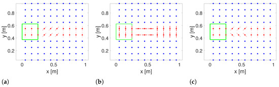
Figure 6.
Examples of simulation layouts for: (a) sorting, (b) slowing or stopping with , and (c) slowing or stopping with .
The second simulated application is the slowing activity. The rotor arrangement consists of a few modules within a line to create a controllable friction on the object to modulate its speed, without pushing it to the sides. The layout in this case can use rotors oriented with their axes in the direction of the flow () (Figure 6b) or inclined at in a row and in the other (Figure 6c).
The last application concerns stopping the motion of an object. This task is the extreme application with respect to the previous application of slowing down. In fact, the modules are still placed with their axes in the flow direction (Figure 6b) or oriented at (Figure 6c), but aim to stop the object.
These three types of simulations do not yet include either real-time control of the rotors or position or trajectory tracking for the object, because, as already indicated, the authors’ objective in this paper is to verify the mechanical functioning of the surface. However, it is possible to imagine that by having sensors that recognize the object arriving at the surface, the modules can pre-arrange the rotors, as shown in Figure 6, depending on the application or sorting direction. This lays the foundation for using the system as a smart surface.
Figure 6 introduces the symbols used in the following sections to display the layouts of the simulations implemented in MATLAB: the red elements correspond to the transport line, the blue dots correspond to the area (array of support points) out of the line, and the green square contour corresponds to the object base. Regarding the transport line, dots represent rotors centers, and lines represent the rotors axes. The red lines before the active area (the green square) are oriented perpendicularly to the flow line and their effect is to reduce in a minimum way the motion of the box in the flow direction, and the inclined lines () simulate the sorting, the slowing, or the stopping surface.
The fixed initial parameters, which are used in all the simulations, are shown in Table 1. In particular, the first four parameters are about the dimension and the inertia of the object, whereas the following three are the friction coefficients. These last values have been chosen by making the following considerations: must be a medium-high friction value (assumed , because is similar to the kinetic friction coefficients between paperboard and the conveyor belt in [42,43]), as it models the sliding of the object on the rotor in the direction of the axis; must be a low value (), as it models the rotational friction of the rotors (assumed , similar to a rolling friction coefficient); and, has to be a low value as well ( is selected), as it models the area outside the line where one can imagine having load-bearing spheres supporting the material (according to the Omnitrack catalog [44], ). Actually, the coefficients described would depend on the materials in contact, which have not yet been defined. However, the exact values are not relevant for the purpose of proving the surface capabilities; the important thing is that is maintained. Finally, the last parameters are the distances in the x and y directions between two rotors centers and the object initial position and acceleration. Exceptions to these starting conditions are indicated with the results for each particular case, together with the missing parameters such as initial velocity of the object and the inclination of the surface .

Table 1.
Initial fixed parameters for the MATLAB simulations.
5. Results
This section presents the simulation results for all three categories: sorting, slowing, and stopping. For each category, the authors illustrate their results for relevant parameter sets and indicate a practical use of the program for the real setup design.
5.1. Sorting
This subsection reports the results of the first of the three categories, sorting. Initially, graphical examples of the function under varying input conditions are shown, then an application for the design of the actual system is presented, and finally a comparison with existing sorting systems is given. Figure 7a,b show the sorting towards the two directions, and , respectively, with an initial object velocity m/s and without surface inclination. Figure 7c, on the other hand, shows the sorting at different tilting angles of the surface and without an initial velocity. Each plot displays the trajectory of G (object’s center of mass) during the sorting and the position and orientation of the object at the end of the simulation time.
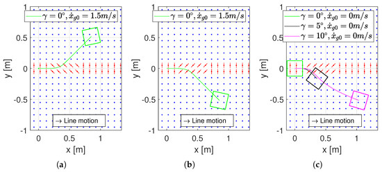
Figure 7.
Illustration of the trajectories and the final position and orientation of the object during: (a) the sorting towards (up) task, (b) the sorting towards (down) task, (c) the sorting towards (down) with different .
In Figure 7a, the green square and its trajectory show that, with rotors inclined at , sorting towards can be achieved, as the object is shifted completely off the line.
The opposite sorting condition was tested as well; the only difference for the initial data was the direction of the rotors (°). The result is shown in Figure 7b and the trajectory is mirrored to the first one. In fact, as expected in reality, the ending displacements of the object are equal in modulus and with opposite sign for the y and displacements (Table 2).
Table 2.
Specific initial data and results for the sorting simulations.
Figure 7a,b show the capability of the surface to deflect the object trajectory for sorting purposes. Furthermore, coherent results were achieved for both sorting directions, for a reasonable initial velocity, and within one second of simulation time. From now on, since the mirroring of the results has been demonstrated for a symmetric rotor arrangement, the outputs are shown only for one sorting direction.
After this first presentation of the sorting capability for the under-actuated system, instead of using an initial object velocity on a horizontal surface, the sorting task was studied with an initially stationary object on an inclined surface with the identical rotor arrangement (Figure 7c).
In Figure 7c, the first case (green) proves that, without any external actuation, the object is not moving in the simulation, as in the real word. In the second case (black square, Figure 7c), with the surface inclination of , the body moves, but for the chosen simulation time ( s) it has not yet completed its sorting. This can be seen from the fact that the black square contour still contains the center of a sorting rotor (red). Finally, the third case (magenta square), where the surface inclination is , reports a completed sorting activity. Summarizing the black and magenta bodies in Figure 7c demonstrate that it is possible to transport and sort parts by inclining the surface. In particular, the more it is tilted, the faster the object moves, and the quicker the sorting is achieved. In Figure 7c, the values of the position and orientation reached at the end of the simulation ( s) for the case (black line) are m m] (Table 2), while those of the magenta line for the same value of m are m m] and the simulation time for which they are obtained is s. Comparing these values, it can be seen that when the surface is more inclined (magenta line), it requires more space in the x direction to perform the sorting , but the time required is less s. In addition, different also produce different final orientations, in this case smaller for larger : .
Table 2 summarizes the results and the initial data about the previous sorting simulations.
A practical use of the simulation is to determine the minimum number of modules necessary for sorting before building the real system. In general, as it was already presented, this result is affected by various initial conditions. However, it can be interesting to know how many columns of rotor units are necessary to successfully complete the different tasks for different object sizes and velocity ranges. In order to derive this relationship, a set of simulations can be performed. Table 3 reports the results of the discussed analysis for two object sizes: m m, called “S-box”, and m m, called “B-box”. “B-box” and “S-box” have the same mass ( kg) and height ( m).
Table 3.
Minimum number of rotor columns required to achieve sorting with °, but changing .
The counting of the number of columns for the sorting is done starting from the first column with the inclined rotors to the last one touched by the object before being out of the line. As is visible from Table 3, the sorting with low initial velocities is not always possible: with less than m/s for “S-box” and less than m/s for “B-box”, the boxes come to a stop within the transport line. Despite this, the speed values considered in the simulations are within the most common operating ranges of conveyors; however, any speed can be implemented in the software. In general, the missed sorting occurs because the deflecting forces also tend to slow the object, which may stop before reaching the target. In addition, the displacement to achieve to be out of the line is related to the dimension of the object, so the bigger it is, the more absolute transversal displacement is required to achieve the sorting. Summarizing, thanks to the simulation described, it is possible to realize such tables depending on the specific application, considering that the results are influenced by the layout of the modules and the initial position. In particular, for Table 3 the “S-box” layout is the same of the sorting simulations of Figure 7b, but with more columns of sorting rotors in order to test a bigger range of velocities. Instead, for the “B-box” there are two more rows of rotors in the sorting line, always with the rotors oriented for sorting towards (), making a total of four instead of two lines.
The data from the simulations carried out to produce Table 3, coupled with further simulations with, as input, only the inclination of the surface, allowed for a comparison of performance with similar existing sorting systems [45]. Figure 8 presents these results. The red dots represent the values of the sorting rate when only the initial velocity is set as input, whereas the blue dots are for when only the inclination of the surface is exploited. Figure 8 shows the most common sorting capacity ranges [45] and, as can be seen, the system proposed by the authors guarantees a medium rate for most input values, with few exceptions in both directions, i.e., high capacity and low capacity. The rate is defined as objects sorted per hour () and can be easily calculated, considering the time needed to perform the sorting and a successful sorting condition. In practice, the condition of successful sorting is when (for the rectangular shape: ), i.e., when the displacement in the direction y is such that, whatever the orientation of the object, the base is no longer in contact with the sorting rotors. The input velocity values presented in Figure 8 are within the common ranges of use for sorting systems. In particular, Ref. [45] for devices similar to the surface proposed by the authors, but fully actuated and called “Torsional discs”, defines input velocities between and m/s. “Torsional discs” have sorting capacities ranging between 1600 and 4500 pcs/h when the size and weight of the transported objects are comparable to those considered in the authors’ simulations (“S-box” and “B-box” characteristics). The system developed in this paper, although it is under-actuated, also allows sorting rates within the same range, providing good performance and in line with the current technology. Obviously, given the under-actuation, there are minimum input speed thresholds, as shown in Table 3, however, they do not seem to limit the application ranges of the device. Tilting the surface and starting from zero initial speed requires longer sorting times and thus provides lower rates than those with velocity as input. However, according to Figure 8, the inclination also provides a predominantly medium sorting capacity, without the need for a prior conveyor. Therefore, the results obtained from the comparison of sorting performances showed that the surface introduced by the authors, with the advantage of the simplicity of the under-actuation, still guarantees sorting capabilities at the same level as current technology, both using initial speed and surface inclination as inputs.
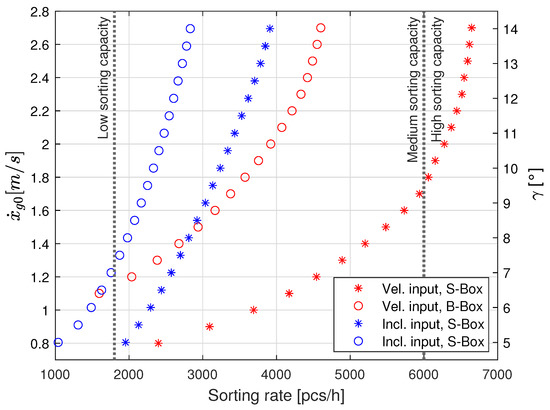
Figure 8.
Sorting rates obtained with MATLAB simulations for the “S-box” and “B-box” objects, with, as input, only initial velocity (red) and only inclination of the surface (blue).
To sum up, the results of this subsection show that the surface is capable of sorting with the two different types of input (Figure 7 and Table 2). In addition, thanks to the developed simulation environment, it was possible to obtain the performance of the system proposed by the authors and compare it with the current technology. This showed that the surface provides a medium sorting capacity (Figure 8), in the same range as existing systems. Finally, for certain objects, the initial input speed was associated with the number of rotors required for sorting (Table 3). This was proposed as a further demonstration of the usefulness of the simulation environment for the design and control of the real system.
5.2. Slowing
The second set of results, here presented, is derived from the slowing simulations. The purpose of these simulations is to simplify and speed up the determination of the number of modules required for the slowing task, which, as with sorting, is linked to the initial parameters. Similar to the sorting results, graphical examples of the functioning and an application for the design of the actual system are given in this subsection.
In order to show the results of the slowing task, in this case the evolution of the object speed over time () is reported. Different from the sorting, here the object is not pushed away from the line, so the trajectory does not represent the course of the activity as simply as speed does. Considering the layout of the system, the only velocity component different from zero is in the x direction, which is the one plotted. Four different setups shown in Figure 9 were simulated to demonstrate the concept’s operation. The graphs in Figure 10a,c show the results of the slowing simulations for the “S-box” and “B-box” cases, respectively.
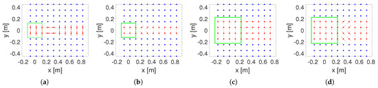
Figure 9.
Layouts of the simulations for the slowing and the stopping tasks with: (a) “S-box” °, (b) “S-box” °, (c) “B-box” °, (d) “B-box” °.
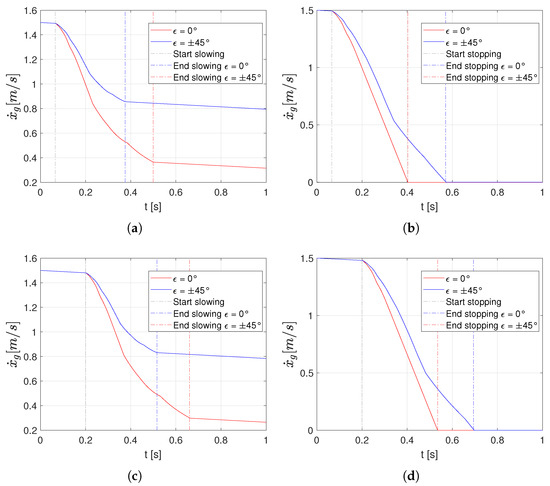
Figure 10.
Velocity trends for “S-box” during (a) the slowing and (b) the stopping, and (c) the “B-box” during the slowing and (d) the stopping with: ° (red), ° (blue).
The initial data for this analysis are the same as in Table 1, with additionally ° and m/s, 0 m/s, 0 rad/s]. As visible from Figure 10a,c, both layouts are capable of reducing the speed of the object, fulfilling the slowing task. However, the speed drop is different with the orientation of the rotors. When the rotors are with °, all the forces in the x direction cause a stronger slowing, whereas with ° layout, where the are inclined like the rotor axes, the slowing is less. For these initial parameters and rotor dispositions, the ratios between the speed before and after the slowing rotors () are: , and , . Additionally, Figure 10 shows the effect of , which is slightly reducing the velocity when the rotors are with °. In fact, the plots in Figure 10a,c show that the lines are a bit inclined before and after the slowing area, which is included between the “Start slowing” and the “End slowing” dotted lines. It represents the contribution of rotational friction to the deceleration.
As for sorting, a parameters study was conducted within the simulation environment to derive the required number of rotor columns to achieve the slow down task of the objects. The results are displayed in Table 4. Additionally in this case, different initial speed and the two different object sizes were tested (“S-box”, “B-box”). The reference layouts for the simulations are the ones in Figure 9. In Table 4, the counting of the columns number begins with the first column with inclination: ° or °, that the object encounters starting from the left. For example, considering Figure 9a and assuming that slowing is verified, the result will be 2 columns (with °). The target condition was set to at least halving the speed of the object while remaining a positive value after the slowing process (). The two configurations (° and °) were possible for the rotor layout, so the configuration with the smallest number of columns was chosen case by case to satisfy the slowing condition. As shown in Table 4 for both layouts and for all speeds analyzed, the number of rotors was identified. The introduction of the ° configuration was necessary, as for some speeds the variant with ° generated a total stop of the conveyed object (e.g., for the first two values in Table 4). The ° positioning also seems promising for the self-alignment of the conveyed material in the center of the transport line. In conclusion, in this subsection, the operation of the surface for slowing tasks was demonstrated (Figure 10). Additionally, as with sorting, certain input speed values of the object were associated with the number of rotors required for the task (Table 4). This provides data for the realization of the physical system and proves the usefulness of simulations for this objective as well.
Table 4.
Minimum number of rotor columns and orientations of their axes () required to achieve slowing () with °, but changing .
5.3. Stopping
The last results, as before, consist of graphical examples of the function and an application for the design of the actual system; however, in this subsection, they are related to the simulations of the stopping condition. In this case, the initial parameters and layouts implemented in the software are the same as before (Figure 9), and only the number of columns of the working rotors changes. Starting from the slowing modules from Table 4 and adding to the right an extra column of rotors with °, the motion of the object can be stopped. The addition of a column proved to be an effective method for simulated speed values; it is not certain that for different values one column is sufficient. Therefore, considering this, Table 4 can also be used for the stopping layout planning. Similar to the slowing, an example (Figure 10b,c) is presented, and only the of the object is reported. However, in this case, the deceleration produced by the rotors of the slowing, plus the extra column, is capable of stopping the object even if the initial velocity simulated is the same as for slowing ( m/s, 0 m/s, 0 rad/s]). In general, according to Table 4 and Figure 10, the size of the object for the slowing and the stopping tasks has less influence than for the sorting (Table 3). This can be seen from the fact that, compared to Table 3, in Table 4, the numbers of columns to slow (then also to stop) the “S-box” and the “B-box” are only different in one case ( m/s). In the end, also for this subsection, the functioning of the surface for the stopping task was demonstrated (Figure 10b,c) and the table with input speeds and number of rotors was explained. Therefore, as final consideration for the whole section, the simulations enable the determination of the layout of the surface, including the module arrangement and the surface inclination for specific applications, while taking the initial conditions of the object into account and which tasks have to be performed. The same MATLAB environment allowed us to obtain the results here presented, proving graphically and numerically the capabilities of the system proposed in this paper.
6. Validation
In order to validate the previous results, this section presents a comparison between the MATLAB environment realized by the authors and a commercial multi-body dynamics software. In the first part of the section, the problem and details on how the validation was carried out are explained, and the second part reports the results.
6.1. Introduction to the Validation
Focusing on the setup of the validation, this subsection is devoted to presenting the objectives, the data, and the ideas behind the comparison. As previously introduced, the sorting system was also modeled in a commercial software for multi-body dynamic simulations: Hexagon D&E Adams MSC. The multi-body dynamic model, called hereinafter Adams for brevity, has two main objectives:
- Providing further demonstration of the functioning of the under-actuated system introduced in this paper;
- Comparing the results with the ones from MATLAB and SIMULINK to have a first validation of the analytical model and the self-developed simulation environment.
Simulations with the Adams software require longer computational time compared to the MATLAB simulations ( s, s, with a HP ProDesk 400 G7). For this reason, Adams was only used for the validation part and not as a standard simulation environment. In fact, using a software as a planning and control tool within the physical system in real time requires very short calculation times, of which the authors’ software is capable.
Figure 11a shows one surface configuration that was previously used in the MATLAB environment for sorting. The identical surface configuration was replicated in Adams, shown in Figure 11b. As it is visible in Figure 11b, the sorting setup was designed in Adams using three different types of bodies: a box (orange wire frame) for the object, cylinders (colorful cylinders) for the rotors, and spheres (pink spheres) for the area out of the line. The chosen inertial and dimensional parameters are shown in Table 5. It should be noted that, for the validation, the values of some inertial parameters are different from previous simulations because the mass properties in Adams were introduced by assigning the material of the bodies. The constraints used for the model are: a fixed joint for the spheres and rotational joints for the cylinders, and the box has contact constraints with the other bodies. The parameters of the contact and the joints are illustrated in Table 6. In particular, for the first five values of this table, the selection was done according to the suggestion of [46,47]: St and Pd are the default values for the contact, whereas kg/s instead of 10 kg/s, Stv and Ftv are smaller than the default (respectively, 100 mm/s and 1000 mm/s) to better simulate the stiction at low speeds. On the same line, the MATLAB parameter, k, of the smooth Coulomb model, is set to to have a similar friction curve. The friction coefficients are the same values implemented in MATLAB, whereas the joint friction parameters are selected to simulate the rotational friction of the joint, similar to the analytic model. To conclude the description, in Adams, the inclination of the surface is simulated changing the gravity vector direction, and the initial velocity is assigned as an intrinsic input condition to the object. Finally, the simulation time considered was s and the step size in the range .
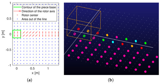
Figure 11.
Model of under-actuated active surface configured for sorting in: (a) MATLAB, (b) Adams.
Table 5.
Inertial and geometrical parameters implemented in Adams for the simulation.
Table 6.
Contact and friction parameters implemented in Adams for the simulation.
The MATLAB setup (Figure 11a) corresponds to the previous sorting setup in Section 5, Figure 7, but in this case it uses the same geometric and inertial data as Adams to simulate the same sorting process. In this way, the results from the two software differ only because of their intrinsic analytic modeling.
After this brief introduction to the Adams model, the simulations performed to meet the two objectives are now described. The configuration with a tilted surface and no initial object velocity was simulated for different angles of inclination ranging from to with an increment of . Additionally, the horizontal configuration () has been simulated with an initial velocity m/s.
6.2. Results of the Validation
This section reports the results of the validation, which are distinguished according to the two objectives of the Adams model. Concerning the first objective, i.e., the proof of functioning of the under-actuated system, Figure 12 graphically reports the results of some Adams simulations. Considering initially only Figure 12a,b, in Figure 12a, sorting is simulated given an initial velocity of zero ( m/s) and an inclination of ; in Figure 12b, the initial velocity is m/s and the inclination is zero (). In Figure 12a,b, it is possible to see the trajectory taken by the G of the object and its final position and orientation given the simulation time of s. The object at the end of the simulation is for both images (Figure 12a,b) outside the sorting zone (zone with cylinders), so the activity is considered completed.
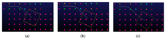
Figure 12.
Object trajectories from Adams with: (a) , m/s, and s of simulation, (b) , m/s, and s of simulation, and (c) , m/s, and s of simulation.
In addition to the case illustrated in Figure 12a, among all the thirty-seven simulations made by varying the inclination of the surface, the ones with (Figure 13a,b) complete the task. For the rest, the target is not really missed, but, because of the limited simulation time ( s), it is not achieved yet. This time was selected because it represents a normal operating condition, for example: there is 1 m of space available in the line for sorting and the conveyor has a speed of 1 m/s. However, as a general rule, when the surface is inclined and with the rotors as in Figure 12, the motion does not self-stop, if . As proof of this, Figure 12c displays the trajectory of the object with ° but s of simulation time, instead of s, and the sorting is clearly obtained. Therefore, the sorting is achievable with this under-actuated system, but it takes time and space. Instead, if the surface is not inclined and there is just the initial speed, the time could be not the only cause of the missed sorting. In this case, the object velocity is inevitably reduced by the friction until the part is stopped, because the gravity is not helping the motion. The same result was highlighted before in the MATLAB environment, which confirms that the simulation environment can be used to predict these conditions.
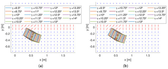
Figure 13.
Final position with in: (a) Adams MSC, (b) MATLAB.
Figure 13 plots the final positions when the sorting is considered achieved for the two software packages (Figure 13a Adams, Figure 13b MATLAB). Having completed the verification of the first objective of the Adams model, it is possible to move on to the second one. Summarizing briefly, objective number two is to exploit the Adams model to show the proximity with the MATLAB results, considering that the same initial data are provided. Figure 14 shows a graphical comparison between the two models referring to the two trajectories of Figure 12a,b. In this case, the trajectories are transposed into a graph (Figure 14) with the corresponding result from MATLAB.
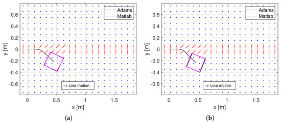
Figure 14.
Comparison of the trajectories with: (a) , m/s, (b) , m/s.
As is visible from Figure 14a,b, the two objects follow very close trajectories and end up almost in the same position and with the same orientation. The absolute and the relative percentage errors obtained for these two simulations are: m, m, °], when the input is °, m/s and m, m, °], when the input is , m/s. The errors are calculated as shown in Equations (5a) and (5b).
The two examples graphically visualize the similarities and the differences between the models. However, to show and summarize all the results for the thirty-seven setups (°°), the final displacements of the Adams and MATLAB simulations together with the errors between them are reported, respectively, in Figure 15 and Figure 16. Considering the x and y results (Figure 15 and Figure 16), the two models (Adams, MATLAB) are not so different, and the relative percentage errors are below and . The trends of the percentage errors seem to have a slight tendency to decrease, and the higher error values occur for small . In contrast, for high values, both coordinates have minimum errors, and . This is because small inclinations generate reduced displacements, especially along y, and the sorting is not completed in the fixed simulation time ( s). This implies that, in the calculation of the percentage error, there are initially very small denominators, and then they become an order of magnitude larger. On the other hand, the absolute errors along values keep oscillating, with a bigger frequency for x and smaller for y.
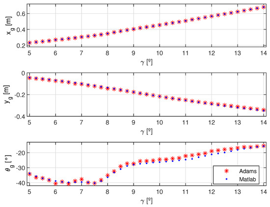
Figure 15.
Final displacements obtained with the two software packages: Adams (red) and MATLAB (blue).
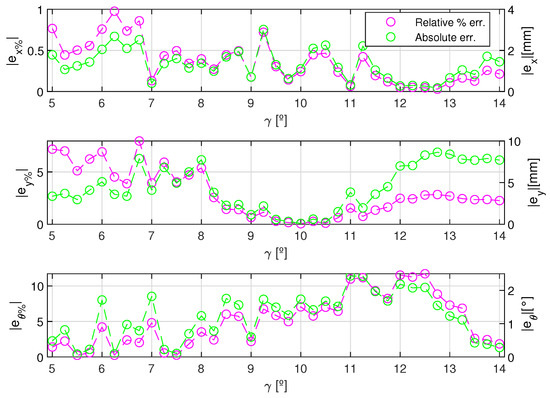
Figure 16.
Absolute (green) and relative percentage (magenta) errors between the final displacements resulting from the two software packages.
For the orientation, higher values are reached () compared to those of x and y. In this case, the phenomenon of the larger percentage error for smaller rotations is not noticed, as in a single simulation there can be counter-rotations, particularly when is big enough to reach the completed sorting area. Thus, the final orientation represents the sum of clockwise and counterclockwise rotations, and its value has not undergone monotonic growth like for the x and y displacements. In general, larger errors of rotations can be explained by comparing how the calculation of normal forces occurs between the two simulations. Adams uses a penetration model to calculate the contact forces, whereas the optimization algorithm (Equation (1)) is implemented in MATLAB. The distribution of normal forces (and therefore also of friction) mainly affects the calculation of the moment, as the position with respect to the pole is important. Whereas, for the x and y displacements, the over mentioned distribution does not have influence, as the resultant force does not change. In addition, an explanation for others slight deviations in trends is the use of different step sizes in some Adams simulations. This was necessary because in a few cases the specific step size chosen was creating a numerical problem, preventing the completion of the simulation. In conclusion, however, the errors are limited and the two models behave in a similar way, thus giving value to the results provided by MATLAB.
To quantify how different MATLAB and Adams values are, the mean values and standard deviations (SD) of the two types of error are listed in Table 7 for the different displacements.
Table 7.
Mean and standard deviation of the relative percentage and absolute errors obtained from the difference between Adams and MATLAB simulations.
As results from Table 7 show, the errors of x and y displacements are very limited. This guarantees that the placing made by the real system can be foreseen in advance with an accuracy appropriated to the applications, so when the sorting line is designed, the simulation can be used to define the layout. For the rotation, the errors are bigger, but, despite this, for a simple sorting operation the final orientation is not interesting, so the MATLAB model can be considered reliable. Furthermore, if in a hypothetical application, the errors allowed are the in the range of those shown in Table 7, the model provides usable results. Concerning that, in many cases it is simply important that the object is not rotated by 180 or 90 with respect to the desired condition.
7. Conclusions
In this paper, the authors present a new modular surface for several intra-logistical tasks. In contrast to similar existing systems, their surface is under-actuated, in particular, composed of idle instead of actuated rotors, whose axes can be fixed in defined, discrete positions within the surface plane. The surface can be used in a horizontal orientation by exploiting an object’s initial velocity, in a tilted orientation by exploiting the gravitational force on the object, or with a combination of both. The authors derived an analytic model and implemented a programmable simulation environment with the software MATLAB for this modular surface. As result, the functioning of the surface concept for the sorting, stopping, and slowing activities was demonstrated, together with the capabilities of the simulation environment. In particular, the MATLAB code showed its potential for predicting, with very short calculation times (≈ or s), the number of modules required for the three handling tasks and how the transported object will behave by simply changing the initial conditions. The same code also made it possible to obtain numerical results of sorting performance and thus have a comparison with current technology, showing that the system proposed by the authors guarantees a medium sorting capacity. These results and examples highlight the usefulness of this environment for real system planning and design. In addition, a validation of the concept and of the simulation environment was conducted with the software Adams. As Adams is a highly sophisticated and well accepted commercial software for dynamic simulations frequently used by engineers to simulate and predict the physical interaction of different components adequately, it is a reasonable tool to be considered as a first reference for the comparison.
In conclusion, the simplifications introduced in the surface, such as the under-actuation and the discrete number of orientations for the rotors, are not limiting the handling capabilities and the performances, but rather they are minimizing the number of constructive components requested and, thus, the costs. In fact, the same goals can be achieved with a reduced design and using in a convenient manner the external actuation, for example, gravity or previous conveyors, already in the line. Additionally, the validation with Adams also showed the accuracy of the main simulation. The differences between the two models are limited and the errors acceptable for many intra-logistics applications. This may open the way to other possible tasks for the surface integrated with the MATLAB environment, such as position and trajectory tracking. In these cases, each time the external environment requires a new position or trajectory of the object, the software calculates the orientation to be given to the rotors. The physical system must be integrated with sensors to adjust in real-time the rotors and achieve the tracking objectives. The implementation of sensors and control strategies for trajectory and position tracking greatly increases the adaptability and flexibility of the system.
No reference is made in the article to construction details in order to keep the validity of the work presented as general as possible. At this point, in order to provide some practical elements and above all to highlight the feasibility of the concept, some schematic solutions are proposed in Figure 17.

Figure 17.
Schematic concepts for the under-actuated module: (a) idle wheel concept, (b) spherical concept.
Figure 17a shows an idle wheel mounted on a vertical axis of rotation. The operating principle is similar to the functioning of a stepper motor, which could be used for this purpose. In contrast, the concept in Figure 17b depicts a spherical rotor whose axis of rotation is locked using mechanically or electro-mechanically driven pins. New tracking objectives, an accurate design, and the control law for the modules are ongoing research topics.
Author Contributions
Conceptualization, E.B., O.J.J., and G.F.; methodology, E.B.; software, E.B.; validation, E.B.; formal analysis, E.B.; investigation, E.B.; writing—original draft preparation, E.B.; writing—review and editing, E.B., O.J.J., G.F., F.J.B.D., and J.A.Y.-F.; visualization, E.B.; supervision, O.J.J., G.F., F.J.B.D., and J.A.Y.-F.; project administration, F.J.B.D. and J.A.Y.-F. All authors have read and agreed to the published version of the manuscript.
Funding
This research received no external funding.
Institutional Review Board Statement
Not applicable.
Informed Consent Statement
Not applicable.
Data Availability Statement
Not applicable.
Acknowledgments
This research work was undertaken in the context of DIGIMAN4.0 project (“Digital Manufacturing Technologies for Zero-defect”, https://www.digiman4-0.mek.dtu.dk/, accessed on 30 January 2023). DIGIMAN4.0 is a European Training Network supported by Horizon 2020, the EU Framework Pro-gramme for Research and Innovation (Project ID: 814225).
Conflicts of Interest
The authors declare no conflict of interest.
Nomenclature
The following nomenclature and abbreviations are used in this manuscript:
| CIR | Center of instantaneous rotation |
| SD | Standard deviation |
| MEMS | Micro electro-mechanical system |
| B-Box | Big box |
| S-Box | Small box |
| Absolute reference frame | |
| Mobile planar reference frame | |
| Absolute reference frame versors | |
| g | Acceleration of gravity |
| m | Object mass, [kg] |
| J | Object moment of inertia, [kg × m] |
| Object base width and length, [m, m] | |
| G | Object center of mass |
| Object center of mass projection on the base | |
| P | Generic contact point between the object and the surface |
| G vertical coordinate, [m] | |
| Vector connecting to P | |
| n | Number of contact points |
| i | Sub-index to indicate the ith contact point |
| t | Time, [s] |
| s | sth step of the loop |
| G coordinates and object orientation, [m, m, rad] | |
| Object velocity components, [m/s, m/s, rad/s] | |
| Object acceleration components, [m/s, m/s, rad/s] | |
| G initial ( s) coordinates and object orientation, [m, m, rad] | |
| Object initial ( s) velocity components, [m/s, m/s, rad/s] | |
| Object initial ( s) acceleration components, [m/s, m/s, rad/s] | |
| Object velocity in P, [m/s, m/s] | |
| Object velocity in P along the axis direction, [m/s] | |
| Object velocity in P along the direction perpendicular to the axis, [m/s] | |
| , | Components of , [m/s, m/s] |
| Object velocity along x after the slowing rotors | |
| r | Speed ratio between the velocities after and before the slowing area |
| F | Force, [N] |
| Friction coefficient | |
| N | Vertical component of the contact force between the object and a rotor, [N] |
| Angle between the x axis and the rotor axis, [] | |
| Angle between the x axis and , [] | |
| Difference between and , [] |
| Friction force components of the object-rotor contact, [N, N] | |
| Friction coefficient in the directions parallel and perpendicular to the axis | |
| , | Friction force components of the object–rotor contact in the |
| frame directions, [N, N] | |
| Friction coefficient outside the sorting area | |
| Array of variables | |
| Function to be minimized | |
| Linear equality matrix | |
| Linear equality vector | |
| Lower bounds vector | |
| Upper bounds vector | |
| Absolute error components, [mm, mm, °] | |
| Relative percentage error components | |
| Set of indexes and a one of its generic elements | |
| Set of geometrical parameters and one of its generic elements | |
| th function that is used to define a perimeter of the objet base | |
| Sets of coordinates that represents the perimeter and the area | |
| of the object base |
References
- Fantoni, G.; Santochi, M.; Dini, G.; Tracht, K.; Scholz-Reiter, B.; Fleischer, J.; Kristoffer Lien, T.; Seliger, G.; Reinhart, G.; Franke, J.; et al. Grasping devices and methods in automated production processes. CIRP Ann. 2014, 63, 679–701. [Google Scholar] [CrossRef]
- Kamagaew, A.; Stenzel, J.; Nettsträter, A.; ten Hompel, M. Concept of Cellular Transport Systems in facility logistics. In Proceedings of the 5th International Conference on Automation, Robotics and Applications, Wellington, New Zealand, 6–8 December 2011; pp. 40–45. [Google Scholar] [CrossRef]
- Rizescu, C.I.; Pleşea, A.I.; Rizescu, D. Modular Transport and Sorting System with Omnidirectional Wheels. In Proceedings of the 10th International Conference on Manufacturing Science and Education—MSE 2021, Sibiu, Romania, 2–4 June 2021. [Google Scholar] [CrossRef]
- Uriarte, C.; Asphandiar, A.; Thamer, H.; Thamer, H.; Benggolo, A.Y.; Freitag, M. Control strategies for small-scaled conveyor modules enabling highly flexible material flow systems. In Proceedings of the ScienceDirect, Procedia CIRP Conference on Intelligent Computation in Manufacturing Engineering, Gulf of Naples, Italy, 18–20 July 2018. [Google Scholar] [CrossRef]
- Böhringer, K.F.; Bhatt, V.; Donald, B.R.; Goldberg, K. Algorithms for Sensorless Manipulation Using a Vibrating Surface. Algorithmica 2000, 26, 389–429. [Google Scholar] [CrossRef]
- Böhringer, K.F. Programmable Force Fields for Distributed Manipulation, and Their Implementation Using Micro-Fabricated Actuator Arrays. Ph.D. Thesis, Cornell University, Ithaca, NY, USA, 1997. [Google Scholar]
- Konishi, S.; Fujita, H. A conveyance system using air flow based on the concept of distributed micro motion systems. J. Microelectromechan. Syst. 1994, 3, 54–58. [Google Scholar] [CrossRef]
- Kritikou, G.; Aspragathos, N. Activation Algorithms for the Micro-Manipulation & Assembly of Hexagonal Microparts on a Programmable Platform. In Advances in Service and Industrial Robotics: Proceedings of the 27th International Conference on Robotics in Alpe-Adria Danube Region (RAAD 2018), Patras, Greece, 6–8 June 2018; Springer International Publishing: Berlin/Heidelberg, Germany, 2018. [Google Scholar] [CrossRef]
- Oyobe, H.; Hori, Y. Object Conveyance System ” Magic Carpet” Consisting of 64 Linear Actuators—Object Position Feedback Control with Object Position Estimation. In Proceedings of the 2001 IEEE/ASME international Conference on Advanced Intelligent Mechatronics Proceedings, Como, Italy, 8–12 July 2001. [Google Scholar] [CrossRef]
- Piatkowski, T. Analysis of translational positioning of unit loads by directionally-oriented friction force fields. Mech. Mach. Theory 2011, 46, 201–217. [Google Scholar] [CrossRef]
- Tao, S.; Youpan, Z.; Hui, Z.; Pei, W.; Yongguo, Z.; Guangliang, L. Three-wheel Driven Omnidirectional Reconfigurable Conveyor Belt Design. In Proceedings of the 2019 Chinese Automation Congress (CAC), Hangzhou, China, 22–24 November 2019; pp. 101–105. [Google Scholar] [CrossRef]
- Whiting, J.; Mayne, R.; Melhuish, C.; Adamatzky, A. A Cilia-inspired Closed-loop Sensor-actuator Array. J. Bionic Eng. 2018, 15, 526–532. [Google Scholar] [CrossRef]
- Keek, J.S.; Loh, S.L.; Chong, S.H. Design and Control System Setup of an E-Pattern OmniwheeledCellular Conveyor. Machines 2021, 9, 43. [Google Scholar] [CrossRef]
- Krühn, T.; Falkenberg, S.; Overmeyer, L. Decentralized control for small-scaled conveyor modules with cellular automata. In Proceedings of the 2010 IEEE International Conference on Automation and Logistics, Hong Kong, China, 16–20 August 2010; pp. 237–242. [Google Scholar] [CrossRef]
- Böhringer, K.F.; Donald, B.R.; MacDonald, N.C. Programmable Force Fields for Distributed Manipulation, with Applications to MEMS Actuator Arrays and Vibratory Parts Feeders. Int. J. Robot. Res. 1999, 18, 168–200. [Google Scholar] [CrossRef]
- Will, P.; Liu, W. ISI/RR-94-391; Parts Manipulation on a MEMS Intelligent Motion Surface. University of Southern California Marina Del Rey Information Sciences Inst: Los Angeles, CA, USA, 1994.
- Frei, P.U.; Wiesendanger, M.; Büchi, R.; Ruf, L. Simultaneous Planar Transport of Multiple Objects on Individual Trajectories Using Friction Forces; Kluwer Academic Publishers: Amsterdam, The Netherlands, 2000. [Google Scholar] [CrossRef]
- Ataka, M.; Legrand, B.; Buchaillot, L.; Collard, D.; Fujita, H. Design, Fabrication, and Operation of Two-Dimensional Conveyance System With Ciliary Actuator Arrays. IEEE/ASME Trans. Mechatron. 2009, 14, 119–125. [Google Scholar] [CrossRef]
- Becker, K.P.; Chen, Y.; Wood, R.J. Mechanically Programmable Dip Molding of High Aspect Ratio Soft Actuator Arrays. Adv. Funct. Mater. 2020, 30, 1908919. [Google Scholar] [CrossRef]
- Fantoni, G.; Santochi, M. Development and testing of a brush feeder. CIRP Ann. 2010, 59, 17–20. [Google Scholar] [CrossRef]
- Chen, Z.; Deng, Z.; Dhupia, J.S.; Stommel, M.; Xu, W. Motion Modeling and Trajectory Tracking Control for a Soft Robotic Table. IEEE/ASME Trans. Mechatron. 2021, 27, 2667–2677. [Google Scholar] [CrossRef]
- Raptis, I.A.; Hansen, C.; Sinclair, M.A. Design, modeling, and constraint-compliant control of an autonomous morphing surface for omnidirectional object conveyance. Robotica 2022, 40, 213–233. [Google Scholar] [CrossRef]
- Robertson, M.A.; Murakami, M.; Felt, W.; Paik, J. A Compact Modular Soft Surface With Reconfigurable Shape and Stiffness. IEEE/ASME Trans. Mechatron. 2019, 24, 16–24. [Google Scholar] [CrossRef]
- Boutoustous, K.; Laurent, G.J.; Dedu, E.; Matignon, L.; Bourgeois, J.; Le-Fort-Piat, N. Distributed control architecture for smart surfaces. In Proceedings of the The 2010 IEEE/RSJ International Conference on Intelligent Robots and Systems, Taipei, Taiwan, 18–22 October 2010. [Google Scholar] [CrossRef]
- Chen, X.; Zhong, W.; Li, C.; Fang, J.; Liu, F. Development of a Contactless Air Conveyor System for Transporting and Positioning Planar Objects. Micromachines 2018, 9, 487. [Google Scholar] [CrossRef]
- Ku, P.J.; Winther, K.; Stephanou, H.; Safaric, R. Distributed control system for an active surface device. In Proceedings of the Proceedings 2001 ICRA. IEEE International Conference on Robotics and Automation (Cat. No.01CH37164), Seoul, Republic of Korea, 21–26 May 2001; Volume 4, pp. 3417–3422. [Google Scholar] [CrossRef]
- Mita, Y.; Arai, M.; Tixier, A.; Fujita, H. Bulk Micromachined Durable Air-Flow Microactuator Array for Robust Conveyance Systems. In Proceedings of the Transducers ’01 Eurosensors XV; Obermeier, E., Ed.; Springer: Berlin/Heidelberg, Germany, 2001; pp. 718–721. [Google Scholar] [CrossRef]
- Mobes, S.; Laurent, G.J.; Clevy, C.; Fort-Piat, N.L.; Piranda, B.; Bourgeois, J. Toward a 2D Modular and Self-Reconfigurable Robot for Conveying Microparts. In Proceedings of the 2012 Second Workshop on Design, Control and Software Implementation for Distributed MEMS, Besancon, France, 2–3 April 2012; pp. 7–13. [Google Scholar] [CrossRef]
- Turitto, M.; Ratchev, S.; Xue, X.; Hughes, M.; Bailey, C. Pneumatic contactless microfeeder design refinement through CFDsimulation. In Proceedings of the Proceedings of 4M 2007, the Third International Conference on Multi-Material Micro Manufacture, Borovets, Bulgaria, 3–5 October 2007. [Google Scholar]
- Zeggari, R.; Yahiaoui, R.; Malapert, J.; Manceau, J.F. Design and fabrication of a new two-dimensional pneumatic micro-conveyor. Sensors Actuators A-Phys. 2010, 164, 125–130. [Google Scholar] [CrossRef]
- Costanzo, M.; Myers, D.H. Diverting Conveyor with Bidirectional Assist Roller. U.S. Patent 9,156,629, 13 October 2015. [Google Scholar]
- Mayer, S.H. Development of a Completely Decentralized Control System for Modular Continuous Conveyors; KIT Scientific Publishing: Karlsruhe, Germany, 2009; Volume 73. [Google Scholar]
- Kleczewski, L. Weighing and Sorting Roller Belt Conveyor and Associated Method. U.S. Patent App. 16/640,445, 18 June 2020. [Google Scholar]
- Overmeyer, L.; Ventz, K.; Tobias Krühn, S.F. Interfaced multidirectional small-scaled modules for intralogistics operations. Logist. Res. 2010, 2, 123–133. [Google Scholar] [CrossRef]
- Sanghai, R.A.; Saundalkar, P.P.; Mallick, J.A.; Shah, B. Sort X Consignment Sorter using an Omnidirectional Wheel Array for the Logistics Industry. In Proceedings of the 2020 International Conference on Convergence to Digital World—Quo Vadis (ICCDW), Mumbai, India, 18–20 February 2020. [Google Scholar] [CrossRef]
- Bhattacharjee, A.; Lu, Y.; Becker, A.T.; Kim, M. Magnetically Controlled Modular Cubes With Reconfigurable Self-Assembly and Disassembly. IEEE Trans. Robot. 2021, 38, 1793–1805. [Google Scholar] [CrossRef]
- Dang, T.A.T.; Bosch-Mauchand, M.; Arora, N.; Prelle, C.; Daaboul, J. Electromagnetic modular Smart Surface architecture and control in a microfactory context. Comput. Ind. 2016, 81, 152–170. [Google Scholar] [CrossRef]
- Huayu, W.; Shunsuke, Y.; Shuji, T. Fabrication of Multi-Axis Moving Coil Type Electromagnetic Micro-Actuator Using Parylene Beams for Pure In-Plane Motion. In Proceedings of the 2021 21st International Conference on Solid-State Sensors, Actuators and Microsystems (Transducers), Online, 20–25 June 2021; pp. 667–670. [Google Scholar] [CrossRef]
- Tisnés, S.D.; Petit, L.; Prelle, C.; Lamarque, F. Modeling and Experimental Validation of a Planar Microconveyor Based on a 2 × 2 Array of Digital Electromagnetic Actuators. IEEE/ASME Trans. Mechatron. 2021, 26, 1422–1432. [Google Scholar] [CrossRef]
- Pennestrì, E.; Rossi, V.; Salvini, P.; Valentini, P.P. Review and comparison of dry friction force models. Nonlinear Dyn. 2016, 83, 1785–1801. [Google Scholar] [CrossRef]
- Green, P.; Worden, K.; Sims, N. On the identification and modelling of friction in a randomly excited energy harvester. J. Sound Vib. 2013, 332, 4696–4708. [Google Scholar] [CrossRef]
- Piatkowski, T.; Wolski, M.; Dylag, K. Angular positioning of the objects by the system of two oblique friction force fields. Mech. Mach. Theory 2019, 140, 668–685. [Google Scholar] [CrossRef]
- Piatkowski, T.; Wolski, M. Model of positioning objects by the system of oblique friction force fields on horizontal and vertically offset planes. Mech. Mach. Theory 2021, 156, 104155. [Google Scholar] [CrossRef]
- Omnitrack. Omnitrack Catalogue. Technical Report. 2022. Available online: https://www.omnitrack.com/wp-content/uploads/2022/11/Catalogue-UK.pdf (accessed on 30 January 2023).
- Piątkowski, T.; Szempruch, J. Ranges of application of sorting manipulators. J. Pol. CIMAC 2011, 6, 235–244. [Google Scholar]
- Verheul, C. ADAMS Methodology Contact Modeling. Benelux ADAMS User Meet. 2012. Available online: https://www.insumma.nl/wp-content/uploads/SayField_Verheul_ADAMS_Contacts.pdf (accessed on 30 January 2023).
- Giesbers, J. Contact Mechanics in MSC Adams a Technical Evaluation of the Contact Models in Multibody Dynamics Software MSC Adams. Bachelor’s Thesis, Faculty of Engineering Technology Applied Mechanics, London, UK, 2012. [Google Scholar]
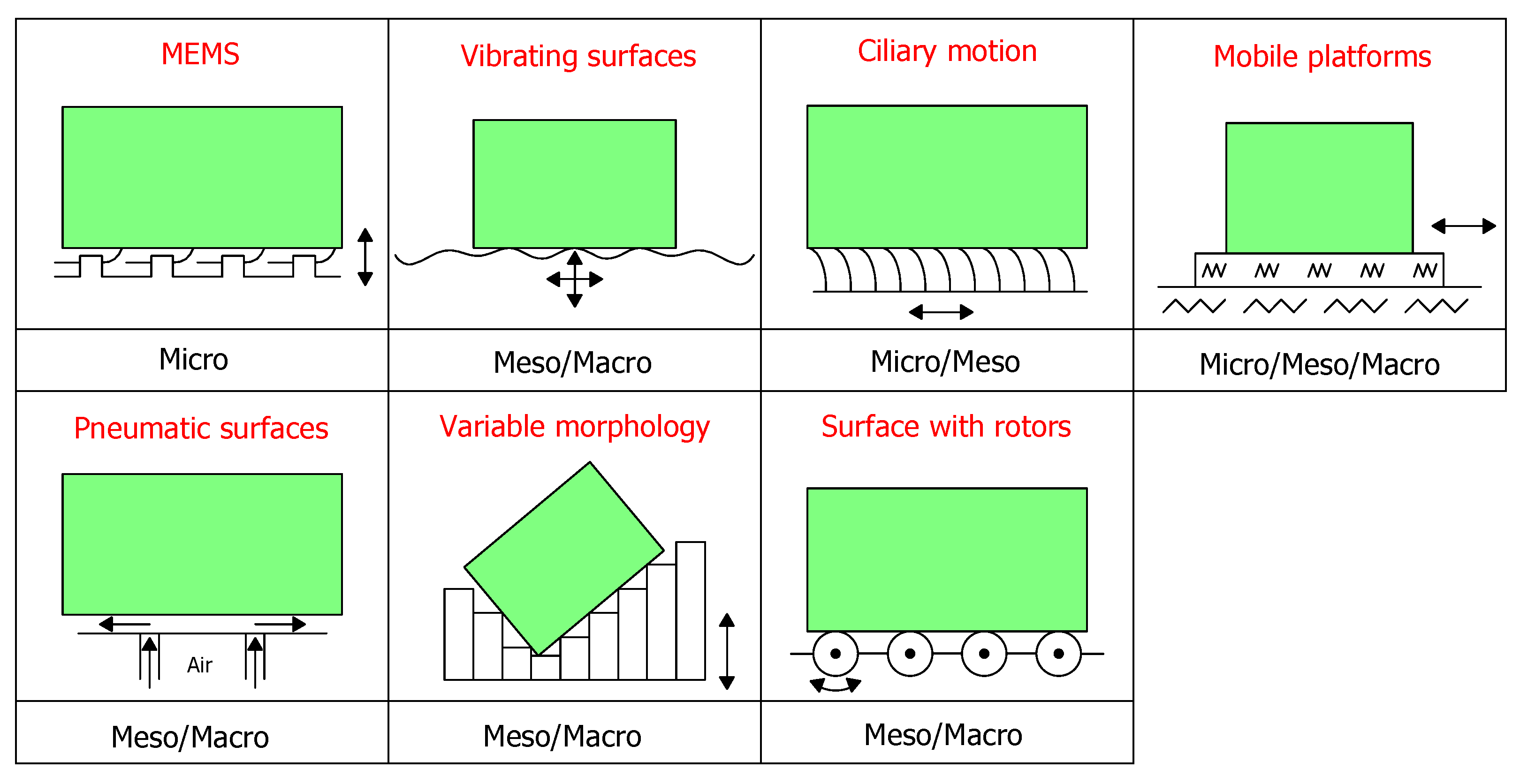
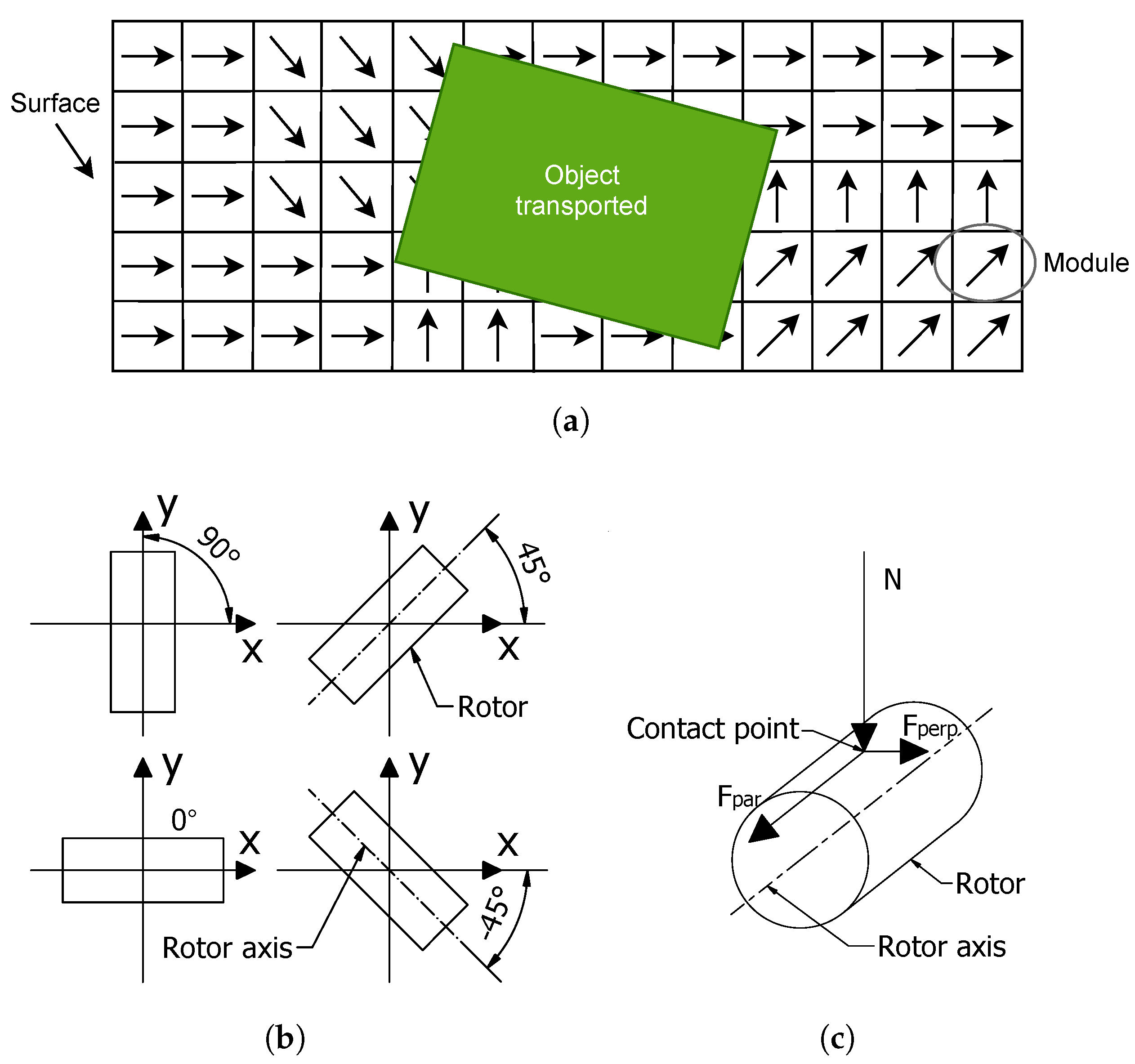

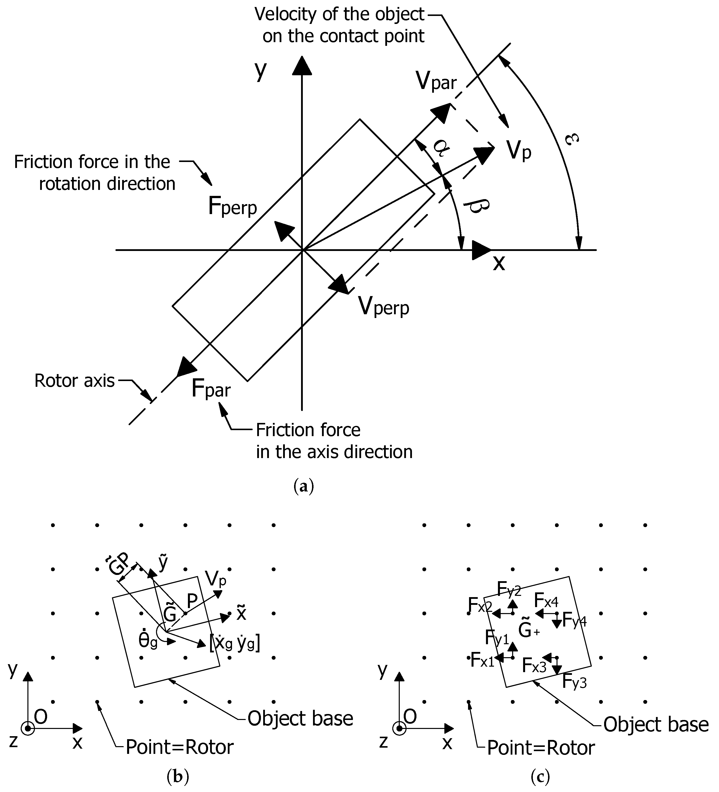
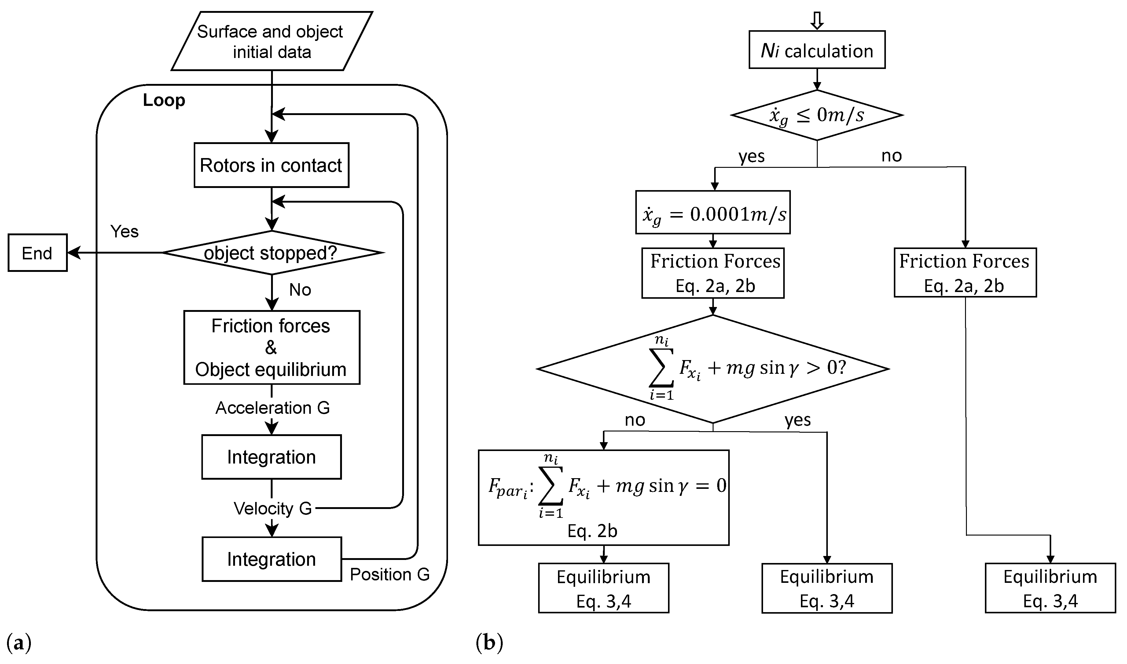
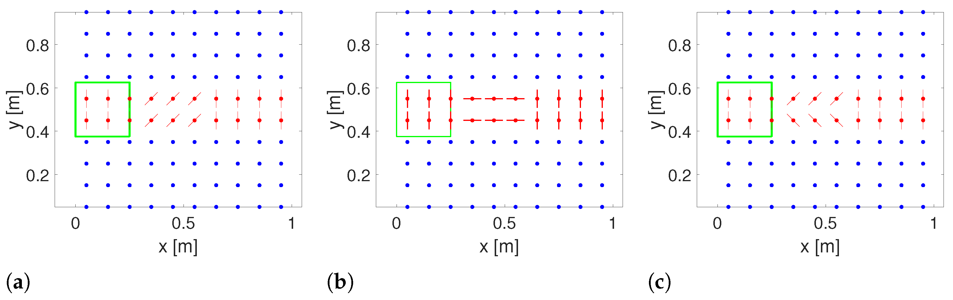
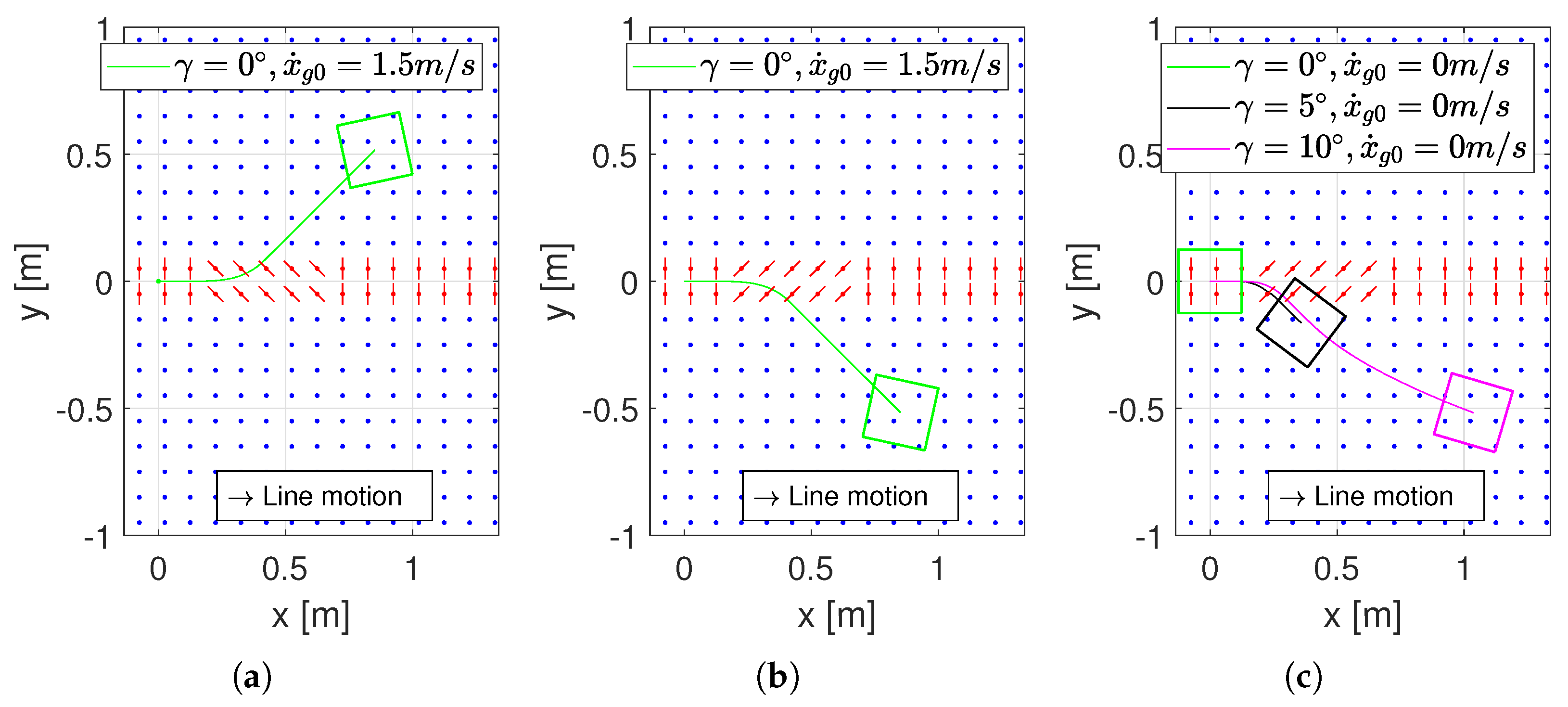
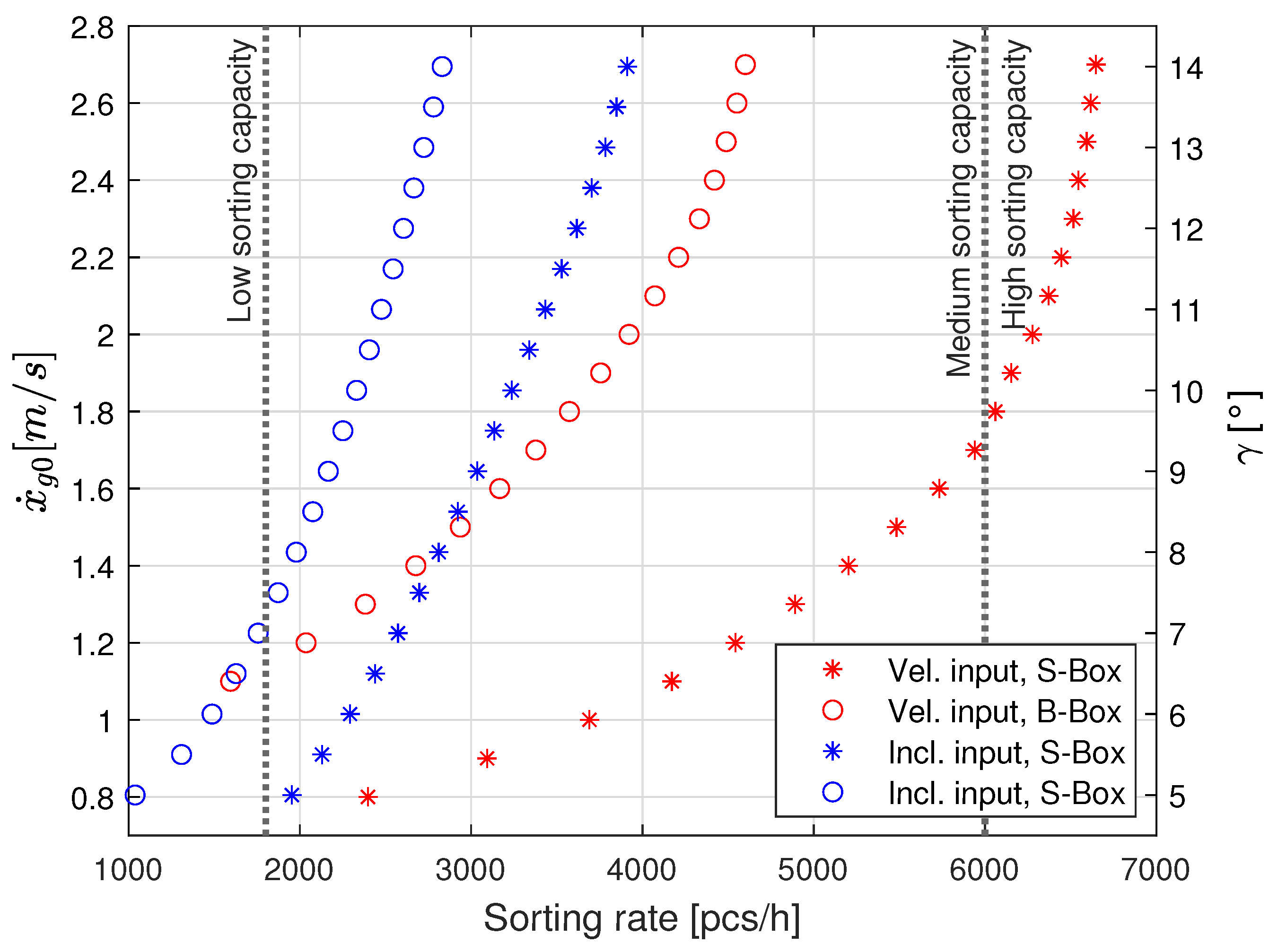
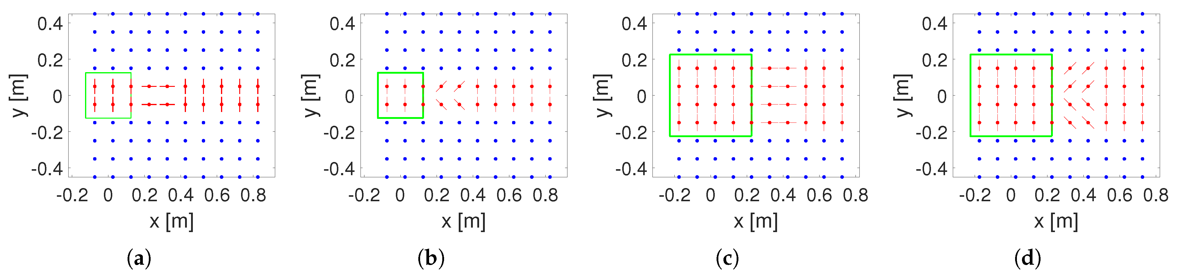
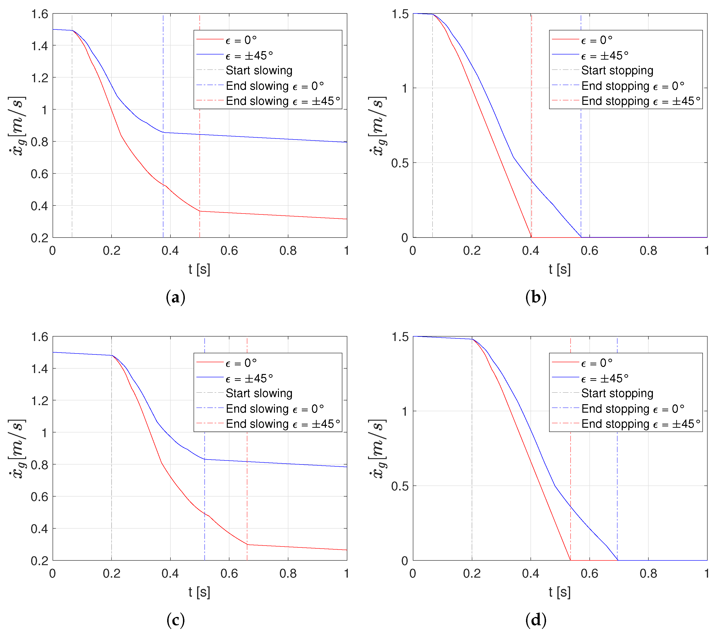
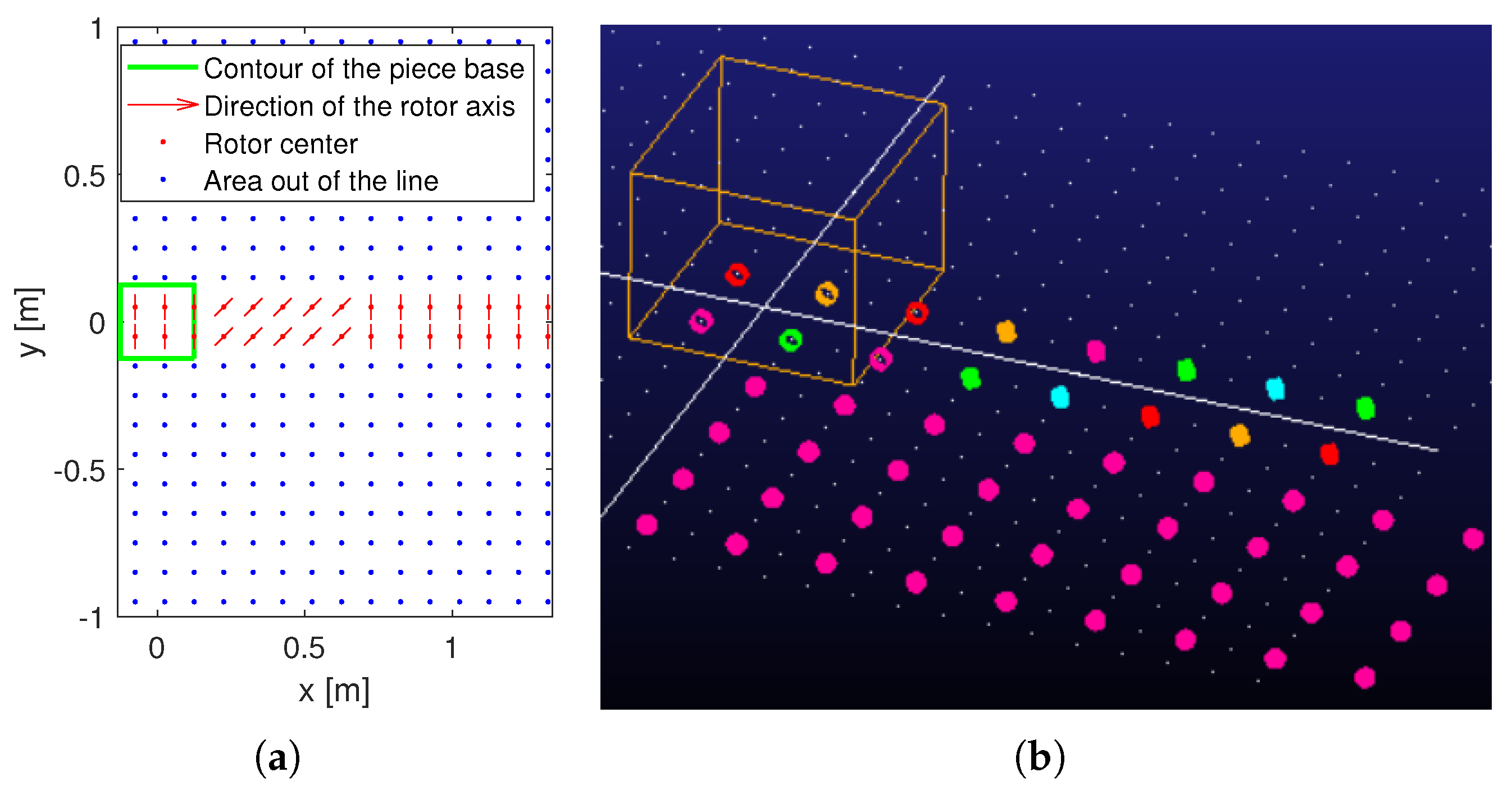
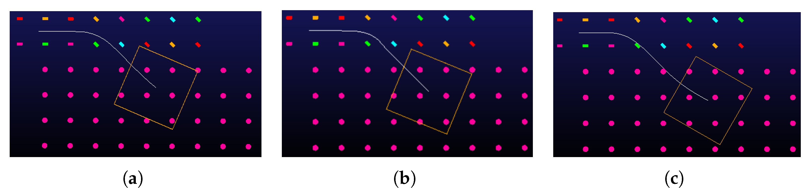
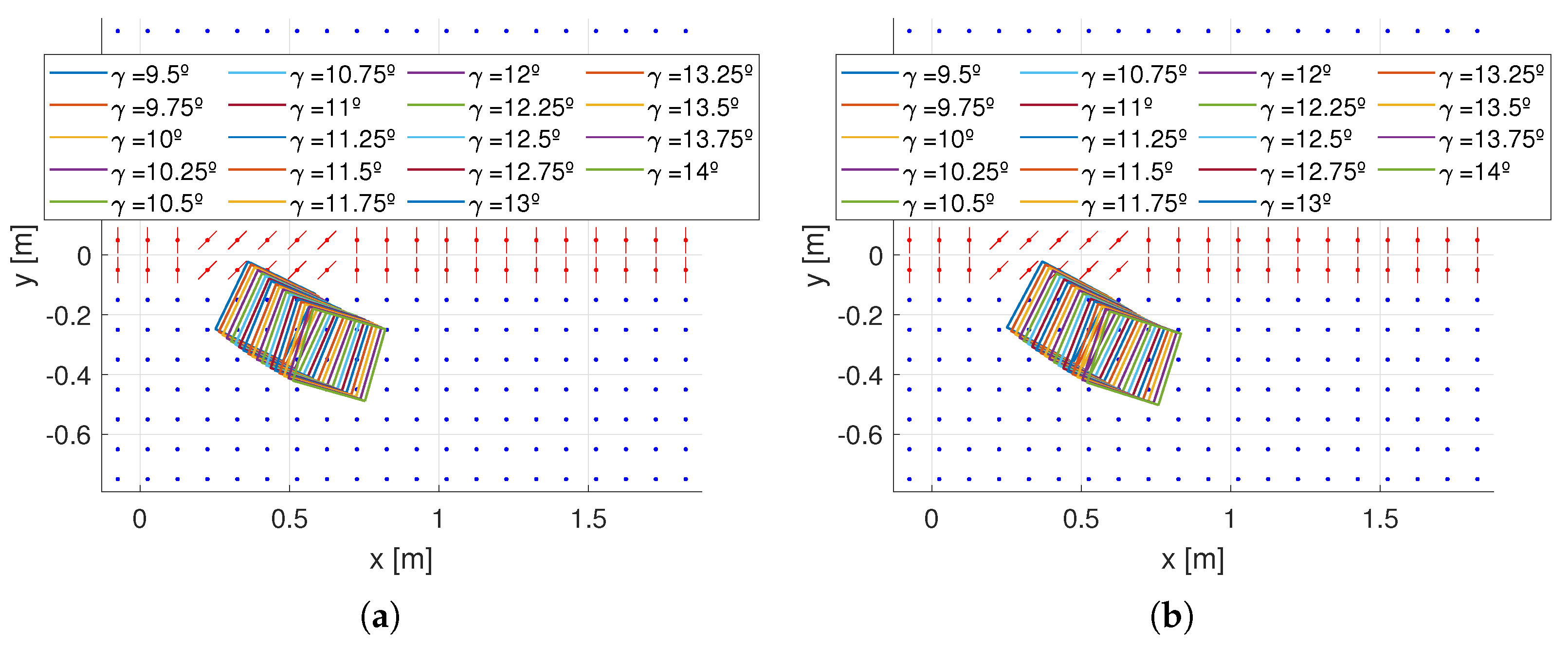
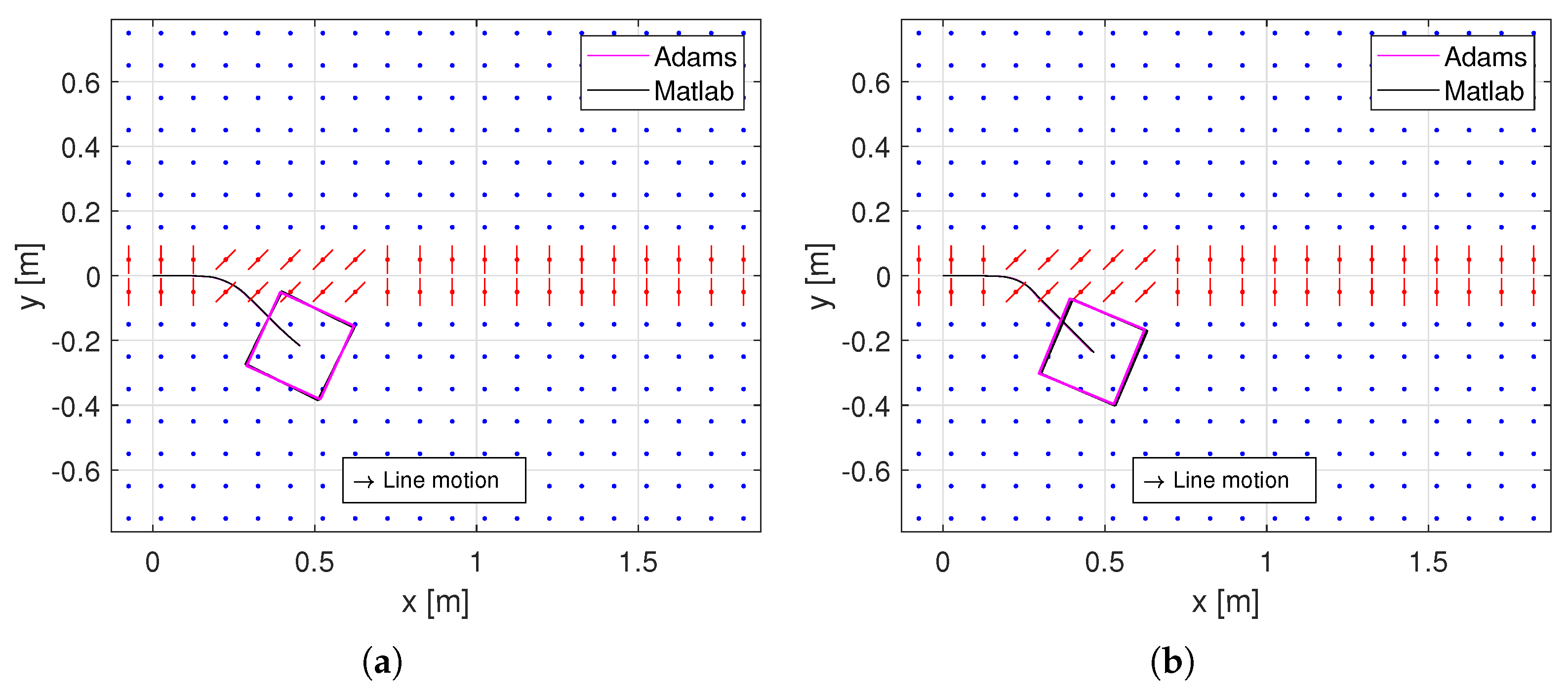
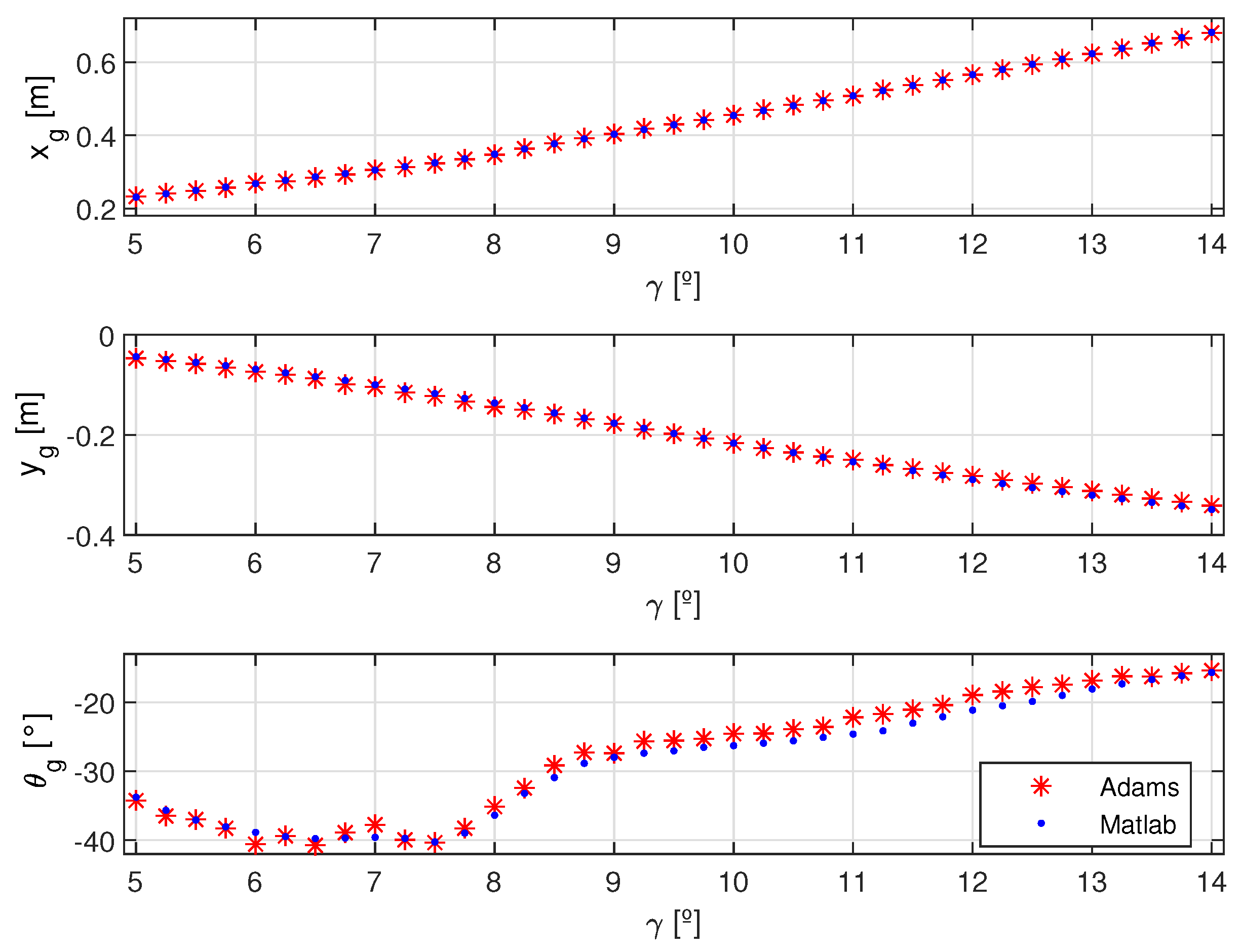
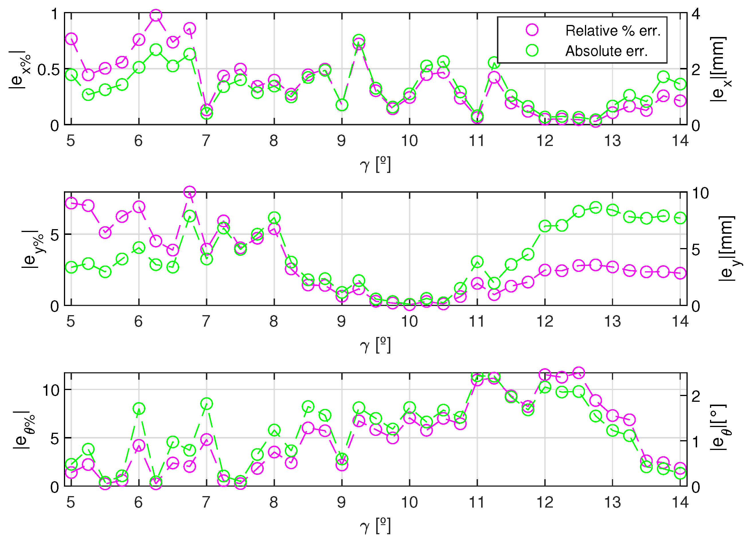
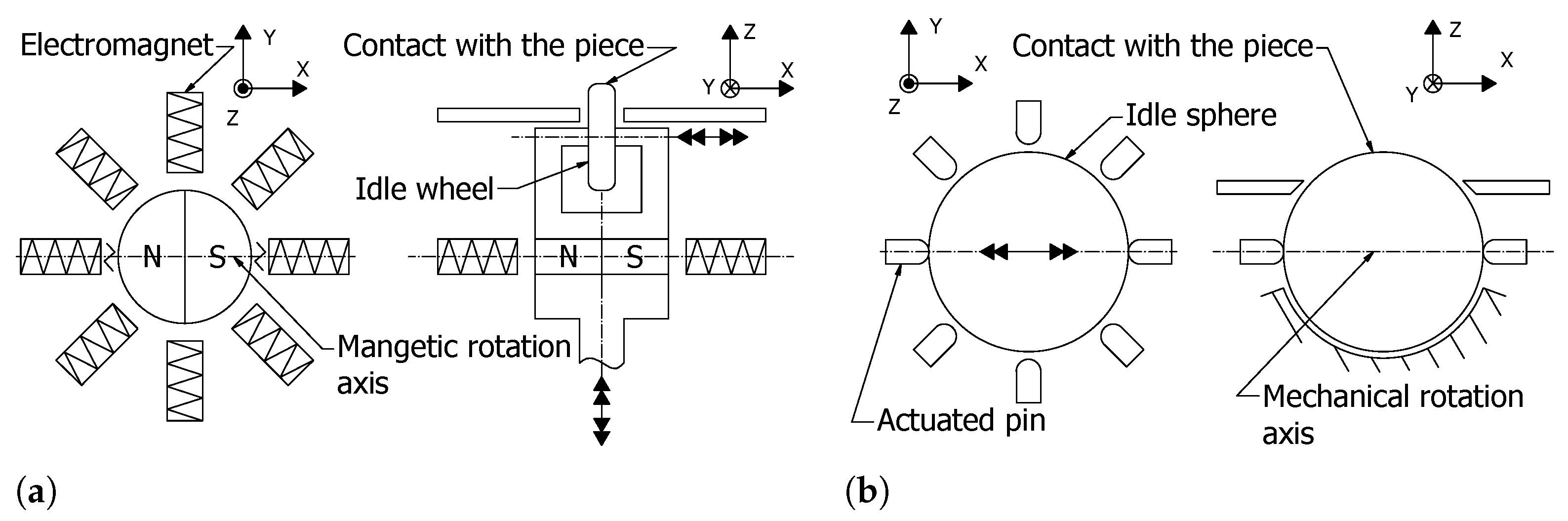
Disclaimer/Publisher’s Note: The statements, opinions and data contained in all publications are solely those of the individual author(s) and contributor(s) and not of MDPI and/or the editor(s). MDPI and/or the editor(s) disclaim responsibility for any injury to people or property resulting from any ideas, methods, instructions or products referred to in the content. |
© 2023 by the authors. Licensee MDPI, Basel, Switzerland. This article is an open access article distributed under the terms and conditions of the Creative Commons Attribution (CC BY) license (https://creativecommons.org/licenses/by/4.0/).