Featured Application
Telepresence robot is useful for remote applications, healthcare and remote sensing.
Abstract
Background: The development of telepresence robots is getting much attention in various areas of human–robot interaction, healthcare systems and military applications because of multiple advantages such as safety improvement, lower energy and fuel consumption, exploitation of road networks, reduced traffic congestion and greater mobility. Methods: In the critical decision-making process during the motion of a robot, intelligent motion planning takes an important and challenging role. It includes obstacle avoidance, searching for the safest path to follow, generating appropriate behavior and comfortable trajectory generation by optimization while keeping road boundaries and traffic rules as important concerns. Results: This paper presents a state machine algorithm for avoiding obstacles and speed control design to a cognitive architecture named auto-MERLIN. This research empirically tested the proposed solutions by providing implementation details and diagrams for establishing the path planning and obstacle tests. Conclusions: The results validate the usability of our approach and show auto-MERLIN as a ready robot for short- and long-term tasks, showing better results than using a default system, particularly when deployed in highly interactive scenarios. The stable speed control of the auto-MERLIN in case of detecting any obstacle was shown.
1. Introduction
The development of telepresence robots is getting much attention in various areas of human–robot interaction, healthcare systems and military applications. The evolution of 6G and 5G also supports these systems and makes them easy to implement. Operating such systems remotely is easy and can be employed in healthcare surgery, and stopping wild forest fires. Many rescue operations use the latest communication technology devices [1]. The prominent areas include healthcare, elderly assistance, autism therapy, guidance and office meetings [1,2,3,4,5,6,7]. The word telepresence [8] means thinking of oneself as being controlled remotely in another environment. The telepresence robots connect through a remote location and receive commands of moving and actuating in that remote location.
Different studies address user-adaptive [2,8] and environment-adaptive systems [9] for human–robot interaction. However, these studies lack many deficiencies in obstacle avoidance and precise self-localization. In the present research work, we further explore the telepresence robots, emphasizing the design of speed control with an additional feature of avoiding obstacles. The mobile experimental robot for locomotion and intelligent navigation (MERLIN) is based on a 40 cm long lightweight chassis and a suspension system, enabling it to drive up to 40 km/h outdoors. Due to its initial purpose, it can be easily equipped with different sensor configurations to characterize the working environment.
In the recent era, telepresence mobile robotics has been expanding rapidly, with a wide range of commercial systems availability and research support [9,10,11,12]. The published work varies from navigation and immersion systems to corporate office and healthcare systems assessments. However, a comprehensive systems design with precision target control is lacking. The main purpose of this paper is to provide a design and analysis of the control systems, their experimental setup, and self-localization with future research directions.
MERLIN is a robotic system based on serious plays for upper limb telerehabilitation in patients with a stroke [13]. It is presented as an affordable and easy-to-use solution to allow the patient to complete intensive rehabilitation at home, with continuous remote monitoring and communication with the therapist [12,13,14]. The system comprises an upper-limb rehabilitation robot and a software platform that guides and measures the patient’s movements and allows physicians to customize the therapeutic plan and monitor the patient’s evolution [15,16].
The purpose of this manuscript is to present the usability validation of the MERLIN system. In this study, we evaluate the ease of use, consistency and acceptance of the system. These systems aim to capture the environment appropriately and to maneuver based on acquired knowledge [17,18,19,20,21]. The main contribution of this paper is to analyze the speed and position controller and stabilize the non-linear behavior by designing an optimized control system. This paper presents and illustrates some ideas that would contribute to the genetic basis of architecture, allowing us to take into account as far as possible the previous requirements. The challenge may be understood as the feasibility of designing an autonomous robot with the capacity to plan its actions to accomplish specified tasks. For that purpose, we emphasize design aspects: speed and control analysis. Furthermore, verification aspects will be made possible almost from implementation up to high-level mission specification when models based on state transition systems are employed.
In the presented research work, a mobile robot based on a chassis of a vehicle model was developed. In particular, a microcontroller-based control was developed, which controls the robot’s behavior depending on user preferences and environmental influences and controls. In addition to the pure control, actuators and sensors, the chassis may be modified or upgraded [22]. This includes small mechanical structures that are necessary. To control the robot’s trajectory, a control program will be developed to evaluate the measured values of various sensors and then spend appropriate control variables on the actuators. In addition, the controller is equipped with a communications interface that allows it to cooperate with a superior level of control. This contains the user program, with which the user can parameterize the robot. The computer also has a wireless interface to operate the robot wirelessly. The basic framework is necessary for the user program, which executes the mini-computer.
Subsequently, the robot’s behavior was examined theoretically. Our findings show that the robot’s safest trajectory settings are determined to apply. Finally, some test scenarios were run with the robot to determine its real behavior for a given trajectory. The desired behavior should be roughly similar [15].
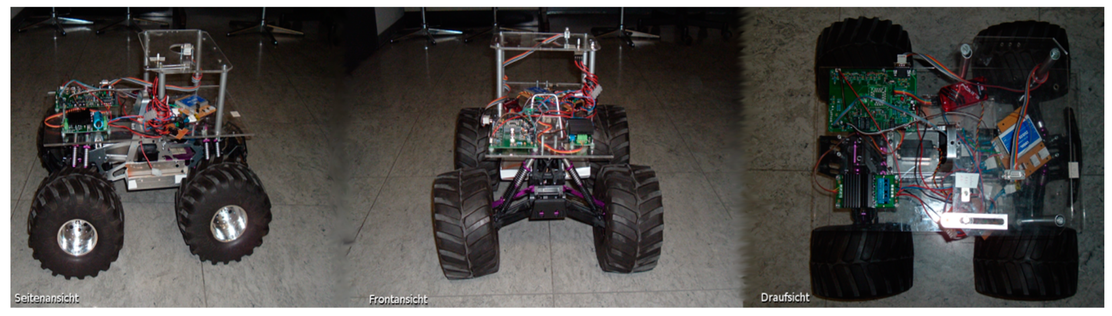
As already mentioned, for this paper, a chassis of a vehicle model type hobby products international (HPI) Savage 2.1 was developed [16]. As shown in Figure 1, a two-track vehicle was equipped with Ackermann steering. It means that the vehicle can drive with only the two front wheels. In addition, the vehicle has four-wheel drive. The force can be transmitted to all four wheels in the same direction. Thus, similar conditions prevail here as in a conventional automobile with four-wheel drive. Turning on the spot is not possible. It follows that the position and orientation of the vehicle are coupled.
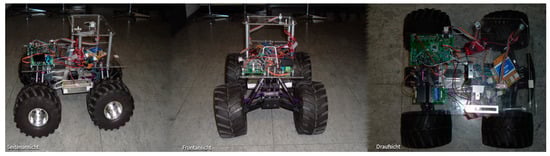
Figure 1.
Monster Truck HPI Savage 2.1 with robot attachment.
The aim should be for the mobile robot to equip MERLIN so that it leaves prescribed paths, navigate, detect obstacles, and avoid them. This required entirely new control electronics to be developed because the old control system did not meet expectations. MERLIN already uses the powerful direct current (DC) motor TruckPuller3 7.2V for the drive and the powerful model-equipped servo motor HiTec HS-5745MG for steering [17]. The drive motor is also equipped with an optical position encoder of the type of the company M101B MEGATRON Elektronik AG and Co, Germany. [18], which the speed and direction can determine.
In Section 2, the background of the study is reviewed, and in Section 3 of this paper, the remote control aspects are addressed in particular, and the modeling and design of the trajectory-controlling algorithm are developed. This is, in particular, used in assembly/disassembly tasks over a given trajectory, where objects are to be pushed by the vehicle toward target locations. Hardware assembling is developed in Section 4. Section 5 presents the results and discussion of the designed control: left/right turn and self-localization.
2. Background
One must choose a technology whose deployment is easy and is quickly understandable by the third-party user. If the user is familiar with the technology and getting acquainted, then no operational manual is required to perform a complex task. This is usually demanded in many fields, including plays, mobile applications, computer programs and robotics. In teleoperating devices such as telepresence robots, the communication interface plays a vital role in controlling the robots [19]. In the healthcare system field, master–slave robots (as a slave) work under the command of an expert (master). The additional usability feature could be an important feature by which many experts from various fields can operate the robots as per their demands or requirement efficiently and flexibly [20,21,22,23,24,25]. The following examples are where experts in many applications can employ these robots.
Medicine is one of the important areas that took advantage of teleoperated systems. The crucial objective is to enhance the performance using the teleoperated robots with good precision and accuracy. These teleoperated robots are becoming more common in microsurgery and minimally invasive surgery [26,27]. Another application area is virtual reality (VR) [27], used for training purposes [28] and simulations [29], which provides more sophisticated knowledge. The military is another area where these teleoperated systems are deployed. The major objective of using robots in this area is to protect human beings from being harmed in high-risk and dangerous situations. To perform such tasks is even crucial, and it is vital to spend less time obtaining the knowledge of the situation [30]. Other similar applications, such as retrieving casualties in battle [10,11,21] or detecting chemicals, gas or radiation [30,31], are also found. Many such systems are employed for many useful purposes, e.g., rescuing people from hazardous situations (fire or collapsed buildings) [32].
Understanding and evaluating the implementation of healthcare interventions in practice is an important problem for healthcare managers and policy-makers [20], and increasingly for patients and others who must operationalize them beyond formal clinical settings [21,22]. Robots are often the only way to explore and manipulate objects in hostile and remote areas. Traditional application areas are space exploration and processing plants for radioactive materials [10]. The advanced concepts for remote control approaches have been realized and are based on combinations of information processing methods with control approaches [23,24]. The increasing capabilities of telematics (telecommunication + informatics) infrastructure, in particular services provided via the Internet, enable nowadays a broad spectrum of commercially interesting applications of these techniques, including telemaintenance of equipment in industrial production or tele-education based on remote experimental facilities [25]. Telematics technologies enable the provision of a continuously growing spectrum of services at remote locations. Major applications are industrial automation, telerobotics for hazardous environments, spacecraft telemetry and telecommand, traffic control, smart homes, tele-education and telemedicine [13,15].
It is known that the necessity of designing truly autonomous robots comes from highly demanding applications (e.g., undersea intervention, planetary exploration, working in nuclear plants, and the coronavirus disease of 2019 (COVID-19)) [12,27,27]. Since when working in such application fields, any repairing intervention is excluded, the need for total technological autonomy is obvious. Furthermore, the dialogue with the end user is reduced to mission specification and, when possible, very few high-level communications. This means almost total operational autonomy is also required, especially in perception, decision and control. This search for functional independence raises major questions in control theory, knowledge-based and reasoning systems, and architecture. However, the specificity of the application domain generates particular constraints, which may sometimes be antagonistic according to the concerned scientific discipline. Historically, many approaches have been developed for performing robot behaviors [3,26,28].
A general hierarchical scheme of autonomous vehicles (AVs) can be found in [29,30]. An AV or robot consists of both software and hardware architectures. Some hardware elements, such as sensors, provide imperative information for the software module [8,12,31]. Furthermore, the software module of AVs generates control commands according to the safety and comfort of the trajectory to the actuator. The actuator controls the hardware activities of AVs, such as steering, acceleration, deceleration, etc. Much research work focuses on identifying and stabilizing the AV and developing a micro-controller-based architecture [10,12,32]. The core responsibility of the design is to control the driving behavior and avoid an obstacle at each instant [8,33,34]. Another important module is the driving behavior planner, which is a decision-making module that provides reasonable obstacle avoidance and safe driving actions [35,36]. Another word, “maneuver,” is also used in the literature for this purpose, but for more clarity and consistency, the term “behavior” will be used to describe it throughout this paper. According to the actions generated by the behavior decision-making module, other independent attributes such as position, trajectory, orientation, and speed are considered [23,37,38]. A popular trajectory definition is a sequence of free-space spatiotemporal states feasible for vehicle dynamics [7,12]. The trajectory control in the software architecture of AVs was presented by [25,39,40,41] in a dynamic traffic environment.
Many trajectory controllers, such as geometric and kinematic, dynamic, optimal, adaptive, model-based and classical controllers, have been implemented for trajectory tracking control [26,35,38,42]. In the past literature, a trajectory planning survey was presented by [13] for autonomous ground vehicles (AGVs), and [43] proposed a comprehensive discussion of motion prediction models and risk estimators. The authors in [44] investigated the functional architecture for autonomous driving and the reasoning for distributing the principal components across the architecture. An overview of the control design methods to handle uncertain forecasts for semi-autonomous and autonomous vehicles was given by [33,37,45,46,47]. From the survey papers, it is easy to conclude that each article investigates individual components such as motion planning, behavior planning, and trajectory control rather than an integrated system [28,44].
One important area is sensor selection and integration. Researchers are exploring using various sensors, such as cameras, lidar, radar and ultrasonic sensors, to detect obstacles and determine the robot’s location. They are also investigating how to integrate these sensors best to provide a robust and reliable obstacle-detection system [48]. Another area of focus is control algorithms. Researchers are developing advanced algorithms that can accurately predict the robot’s motion and path and quickly respond to environmental changes to avoid obstacles. These algorithms typically involve using sensor data to estimate the robot’s state and then using that information to plan and execute safe trajectories [49]. A third area of focus is human–robot interaction (HRI). Telepresence robots are often operated by humans, who may not have much experience with robotics. Researchers are investigating how to make the control interfaces for telepresence robots more intuitive and easier to use to enable more effective human–robot collaboration [50].
In summary, the proposed work is focused on improving the reliability and robustness of the obstacle detection and avoidance system, developing advanced control algorithms that can quickly and accurately respond to changes in the environment and making the control interfaces user-friendly [51].
3. System Design and Implementation
The focus moves in a linear function of the target position between the robot’s orientation at the start of the trajectory and orientation. The following values given in Table 1 are of particular importance:
where this is an angle that must be in the interval [−π; π]. It is, therefore, possible to use modulo 2π arithmetic.

Table 1.
Important parameters of calculation.
The simulated orientation finally calculates to:
As already mentioned, the simulated position and orientation values serve as setpoints for the position and orientation controller, where represents the target position, which is the integration of the target speed. The position controller is implemented as a proportional-integral-derivative (PID) controller with anti-wind-up feedback. On the other hand, the orientation controller controls based on the distance covered, so a proportional-integral (PI) controller with a variable time base is selected here.
In addition to pure position and orientation control, there is obstacle detection and avoidance. It is superimposed on the two controllers and intervenes in the event of an impending collision with an obstacle. The two controllers are frozen because the robot must correct its course after avoiding an obstacle and stops first.
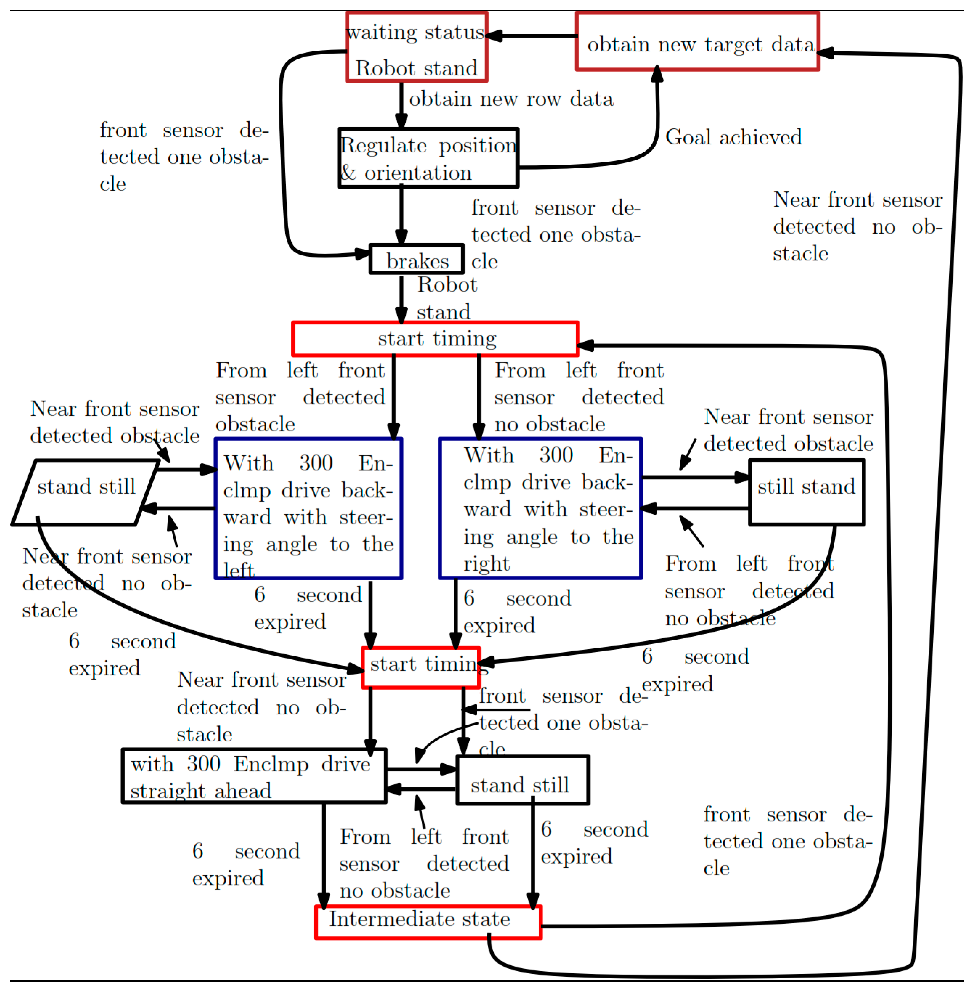
The above-described state machine for avoiding obstacles is shown in Figure 2. If the front sensors detect an obstacle too close, the trajectory run can no longer be continued. Therefore, the robot first stops as fast as the speed controller allows. Then the robot slowly drives backwards for 6 s with the steering turned to the maximum. The steering direction depends on which sensor detected the obstacle. In case the left front sensor detects the obstacle, the wheels are turned to the left; otherwise, the wheels are turned to the right. If one of the rear sensors detects an obstacle, the robot remains standing until the obstacle disappears. For a fixed obstacle, the robot will no longer drive backwards. If an obstacle rushes by, reverse travel is continued after the obstacle has disappeared. It must be remembered that the robot only forgets nearby obstacles after a second. After the time has elapsed, the robot slowly drives straight ahead unless a nearby obstacle is detected by at least one of the front sensors. Otherwise, the robot remains standing, just like when reversing. After 6 s, it is checked whether at least one of the front sensors detects a nearby obstacle. If so, the evasive maneuver described begins again from the beginning. Otherwise, the robot stops and reports to the mini-computer that it has successfully avoided an obstacle. It must then supply new target data, regulation of position and orientation, obstacle detection and avoidance.
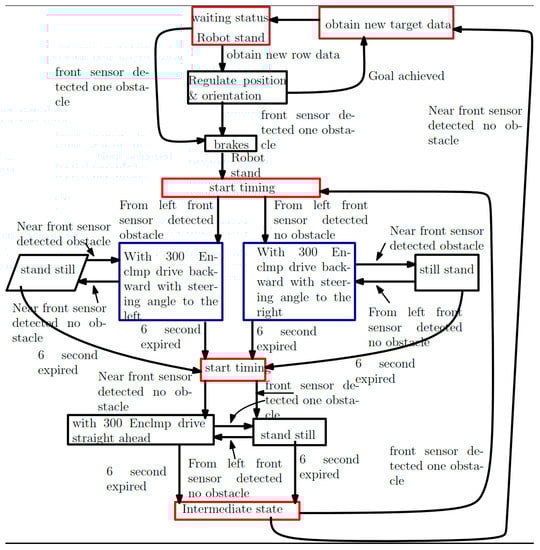
Figure 2.
State machine for avoiding obstacles.
3.1. Speed Control
The speed controller, as shown in Figure 3, controls the speed of the robot’s drive train. The drive consists of two DC motors connected in parallel, transmitting their mechanical power to the drive gear. On the electrical side of the motors, they are fed by the motor controller. The motor controller itself receives the manipulated variable from the controller. The actual value of the drive, i.e., the estimated position of the robot, is recorded by the encoder on the drive gear. This actual position value is differentiated once, smoothed, and finally fed into the control loop. A digital PID controller with anti-wind-up feedback is used as the controller here, but it is only used as a PI controller.
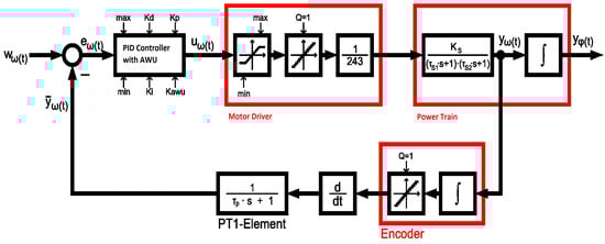
Figure 3.
Speed control loop.
Path planning and self-localization are two important components of telepresence mobile robots. Path planning is determining the best path for the robot to follow to reach its destination while avoiding obstacles and other potential hazards [52]. Path planning algorithms typically use sensor data, such as information from cameras or lidar, to build a map of the robot’s environment and then to plan a safe and efficient path. Some common path-planning algorithms include the A* algorithm, Dijkstra’s algorithm, and rapidly-exploring random trees (RRTs) [53].
Self-localization is the process of determining the robot’s current location within its environment. It is typically done by using sensor data, such as information from cameras or lidar, to compare the robot’s current sensor readings with a pre-built map of the environment [54]. Some common self-localization algorithms include Monte Carlo localization (MCL), extended Kalman filter (EKF), and particle filter [55].
Path planning and self-localization are essential components for telepresence mobile robots, which help it to navigate and operate autonomously. They are typically integrated into a single control system that can make decisions and take actions based on sensor data and the robot’s current location and destination.
It is important to note that both path planning and self-localization are active research areas, and new algorithms and techniques are being developed to improve these systems’ reliability, robustness and efficiency.
The block diagram of the speed control loop is shown in Figure 3, in which we highlight three red boxes. These boxes are replicas of the real technical control of the robot modules. The red box motor driver describes the MD03 motor driver module. The module expects a manipulated variable with values between −243 and 243. The quantizer then quantizes these to integer values. Finally, the output signal is normalized to values between −1 and 1. It is not normalized to the output voltage of the motor driver since it depends on the battery voltage. The battery voltage is considered in the gain of the controlled . The motor driver directly closes the red box on the drive train, whose input variable is the output of the motor driver.
The drive model is approximated as a PT2 element to determine the vehicle speed. This model contains the drive from the battery voltage to the motors and the gearbox to the tires. In particular, this modeling also includes the weight of the robot. A step response experiment determines the parameters , and of the drive train. The integrator following the PT2 element completes the model in that the robot travels a distance. It integrates the speed to a distance.
The red encoder box represents a control-technical simulation of the built-in rotary encoder. The rotary encoder has an integral behavior here since it picks up the speed from the gearing but converts it into a distance during processing. Since the encoder discretely measures the distance covered, it quantizes the distance to whole encoder pulses, i.e., integer values.
The hardware components must be completed with suitable software to form a control loop. First, the encoder position value is differentiated to obtain the robot’s speed. A PT1 element then smooths this value with the time constant to reduce noise. This smoothed value is the actual speed at the setpoint/actual value comparison.
A PID controller with anti-wind-up feedback is used as the controller. The manipulated variable limitation in the controller should correspond to the manipulated variable limitation of the motor driver so that the anti-wind-up feedback can work optimally.
It should be mentioned that angular velocities and angular distances are processed in the controller model. However, these are proportional to the linear speed and distance of the robot. Only the constant of proportionality still has to be determined in an experiment that will be carried out later.
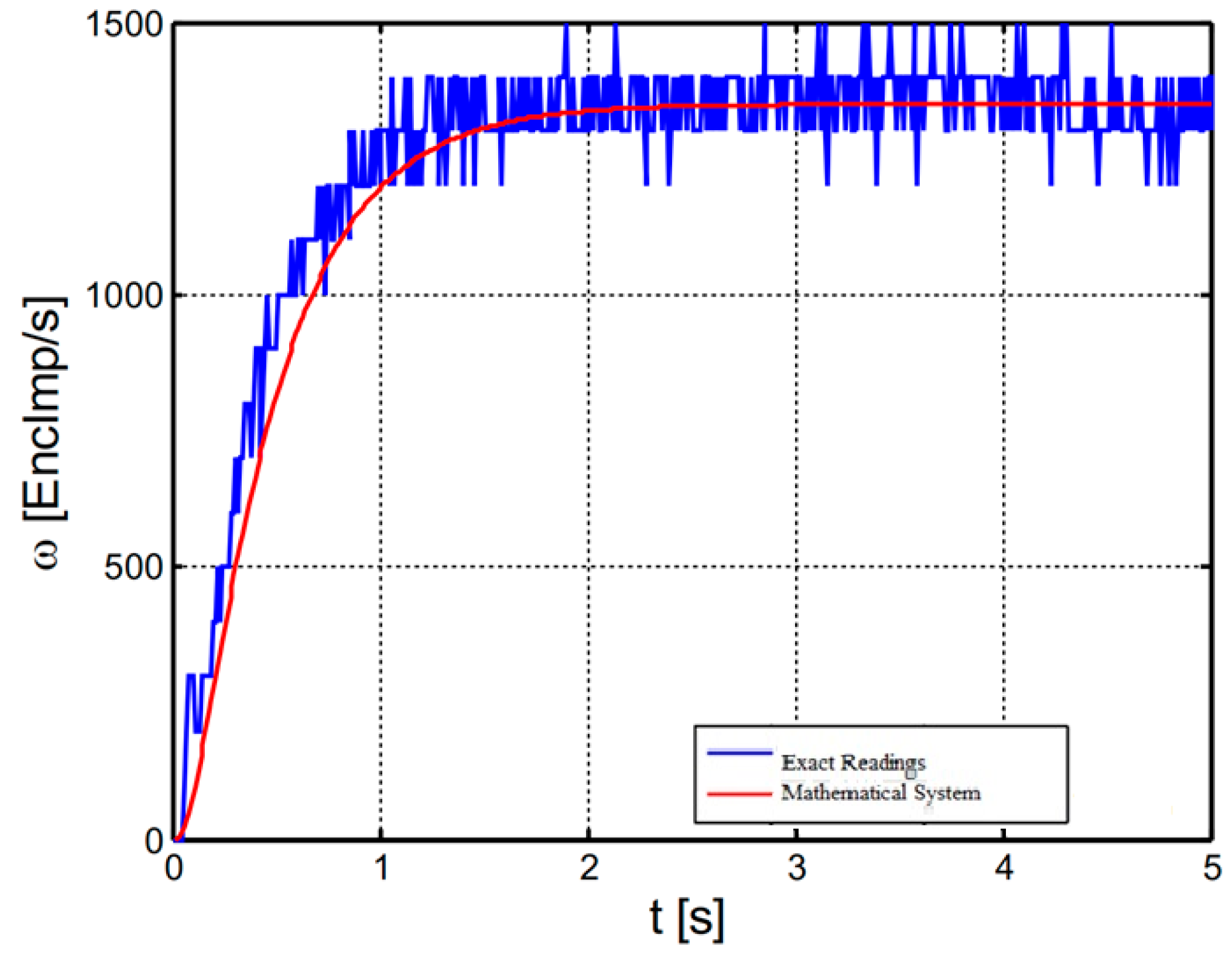
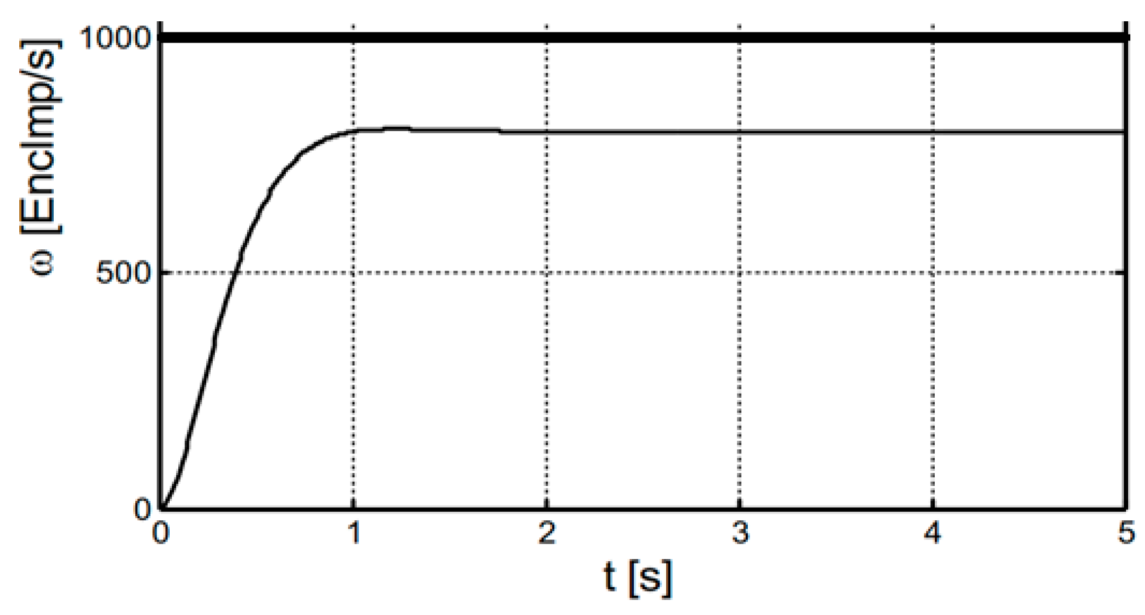
To adjust the control loop, a model of the drive train that is as precise as possible is first required. As already mentioned, the drive is modeled by a PT2 element and subsequent integrator. The parameters are determined by analyzing the robot’s step response. The distance covered is recorded by the robot via the step response function. This recording can then be transferred to a personal computer (PC) for evaluation. However, since the speed step response is sought, the values obtained must be differentiated numerically once. The step response shown in Figure 4 was carried out with two “TruckPuller3 12V” drive motors with a battery voltage of 7.2 V and without a mounted PC. The blue characteristic shows the measured values. The quantization by the rotary encoder can be seen very well with them. The characteristic red curve describes an ideal PT2 element with a gain of = 1350, and the time constants = 0.1 s and = 0.4 s. This element represents a fairly good approximation of the real system.
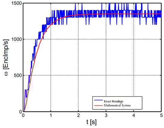
Figure 4.
Step response speed of the robot.
All variables are now known to set the control loop. For the time being, the PT1 element is bypassed in the feedback to make the controller design easier. The PID controller is only used as a PI controller. It avoids erratic behavior of the control loop, which would be problematic anyway due to the limitation of the manipulated variable.
All time constants are represented as poles and zeros in the following derivations:
The drivetrain part relevant to the cruise control is the PT2 element. Its mathematical description is:
The PI controller lets itself through:
with the zero:
For completeness, the transfer function of the PT1 element in the feedback is:
All quantizers and manipulated variable limitations are not considered when parameterizing the controller. As a result, the integrator of the encoder and the subsequent differentiator cancel each other out. This means that only the PT1 element is left in the feedback path.
First, the transfer function of the open loop is determined. The amplification factor of the motor-driver must also be considered.
Now the controller’s zero point is selected so that the slowest pole point is compensated. This simplifies the controller function to:
with:
Since the feedback is bridged, it is sufficient to determine the transfer function of the open loop for the root locus. If one inserts the system parameters determined into Equation (9), one obtains the transfer function of the open control loop:
3.2. Root Locus of Speed Controller
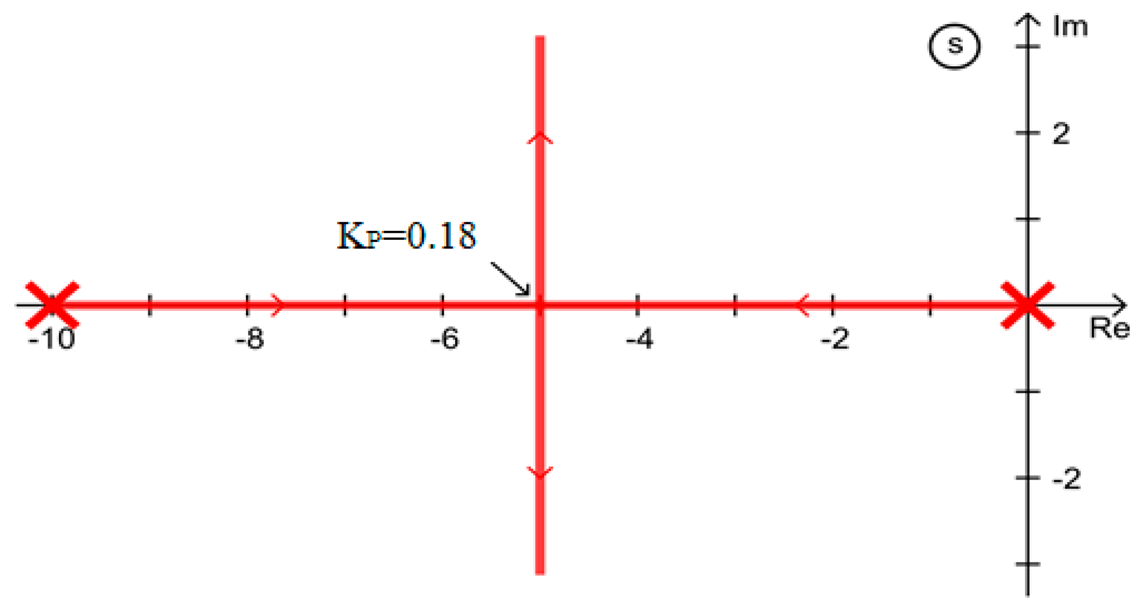
The root locus for this is shown in Figure 5. The aperiodic limiting case occurs at a controller gain of = 0.18. With larger gains, the controller oscillates. The root locus curves were determined using MATLAB’s single-input, single-output (SISO) design tool. If the smoothing in the feedback of the control loop is also considered, the controller receives an additional pole. This also significantly changes the root locus curve. For the controller parameterization, the smoothing has a time constant of = 0.05 s, corresponding to a pole at −20.
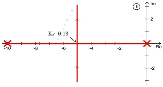
Figure 5.
Root locus of the speed controller without smoothing in the feedback.
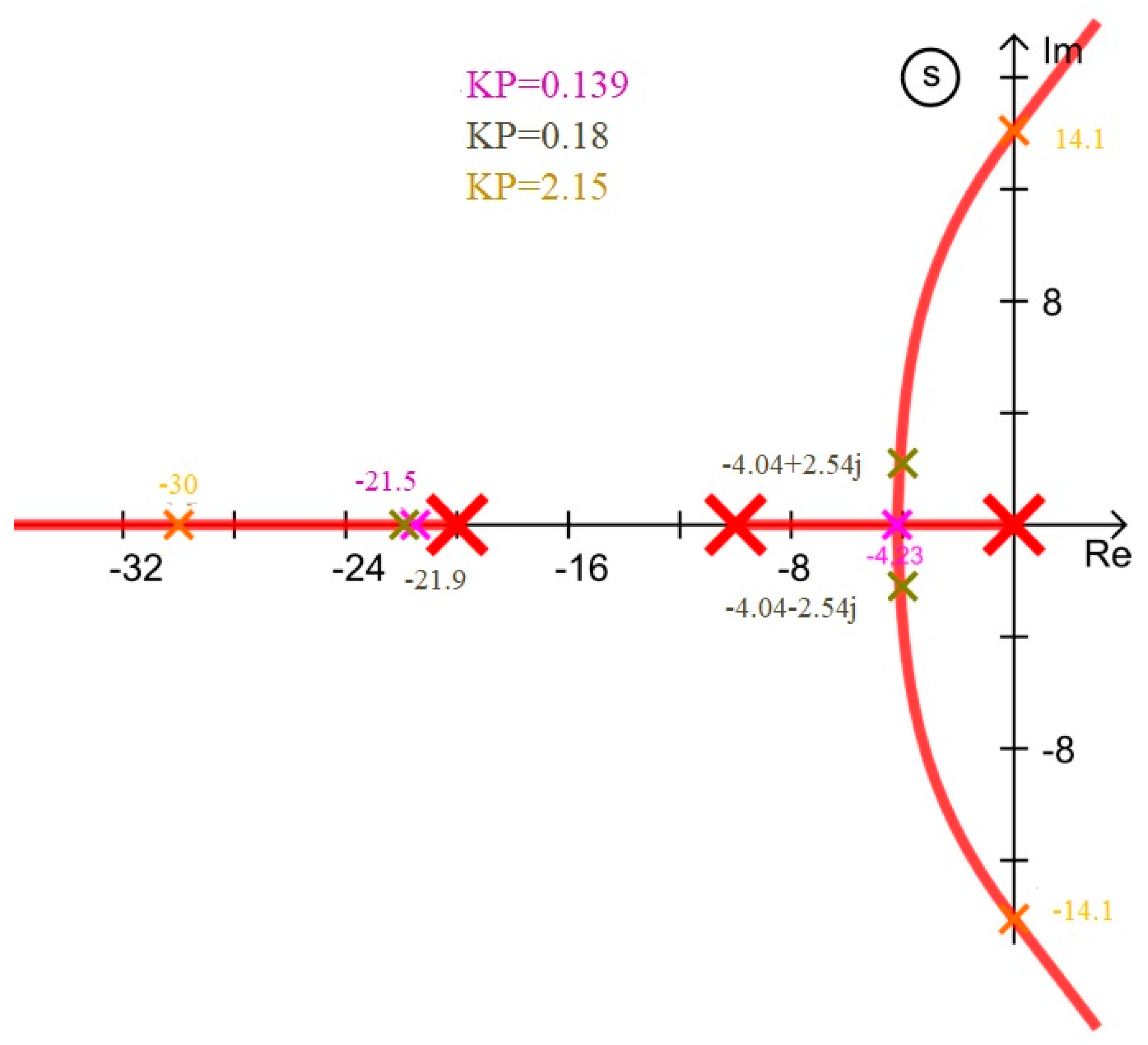
Figure 6 shows the root locus of the new control loop. The poles for distinctive points are drawn in different colors. The aperiodic limit case occurs with a controller gain of = 0.139 (magenta). The stability limit is at a gain of = 2.15 (orange). The amplification of = 0.18 (green) determined in the previous investigation leads to a slightly oscillating behavior.

Figure 6.
Root locus of the speed controller with smoothing in the feedback.
Now the transmission behavior of the control circuit is determined. The open-loop transfer function is unaffected by the smoothing in the feedback, so Equation (9) can still be used for this. However, the transfer function of the closed control loop is relevant for the overall behavior, which is calculated as:
By inserting the individual transfer functions, one obtains:
By solving the double fraction, we obtain:
At this point, the controller gain of the speed controller is set to = 0.18. The control circuit thus has a slightly oscillating behavior. However, it must be noted that the actual value measurement is subject to a large amount of quantization noise. If the oscillation amplitude is below the rotary encoder’s resolution, it is practically non-existent because it cannot penetrate the controller input. Due to the zero point at = = −2.5, the amplification of the integral component is calculated:
This means that all parameters for the speed controller are known. Inserting them into Equation (15) results in the transfer function for this special case of the speed controller.
The poles of the controller are included:
The zero point of the controller corresponds to the time constant of the PT1 element in the feedback.
Figure 7 shows the step response of the speed controller when the speed jumps from 0 EncImp/s to 800 EncImp/s at time t = 0 s. The diagram clearly shows that the system is corrected very quickly. There is a slight overshoot in speed.
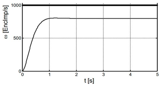
Figure 7.
Theoretical step response of the speed controller (linear model).
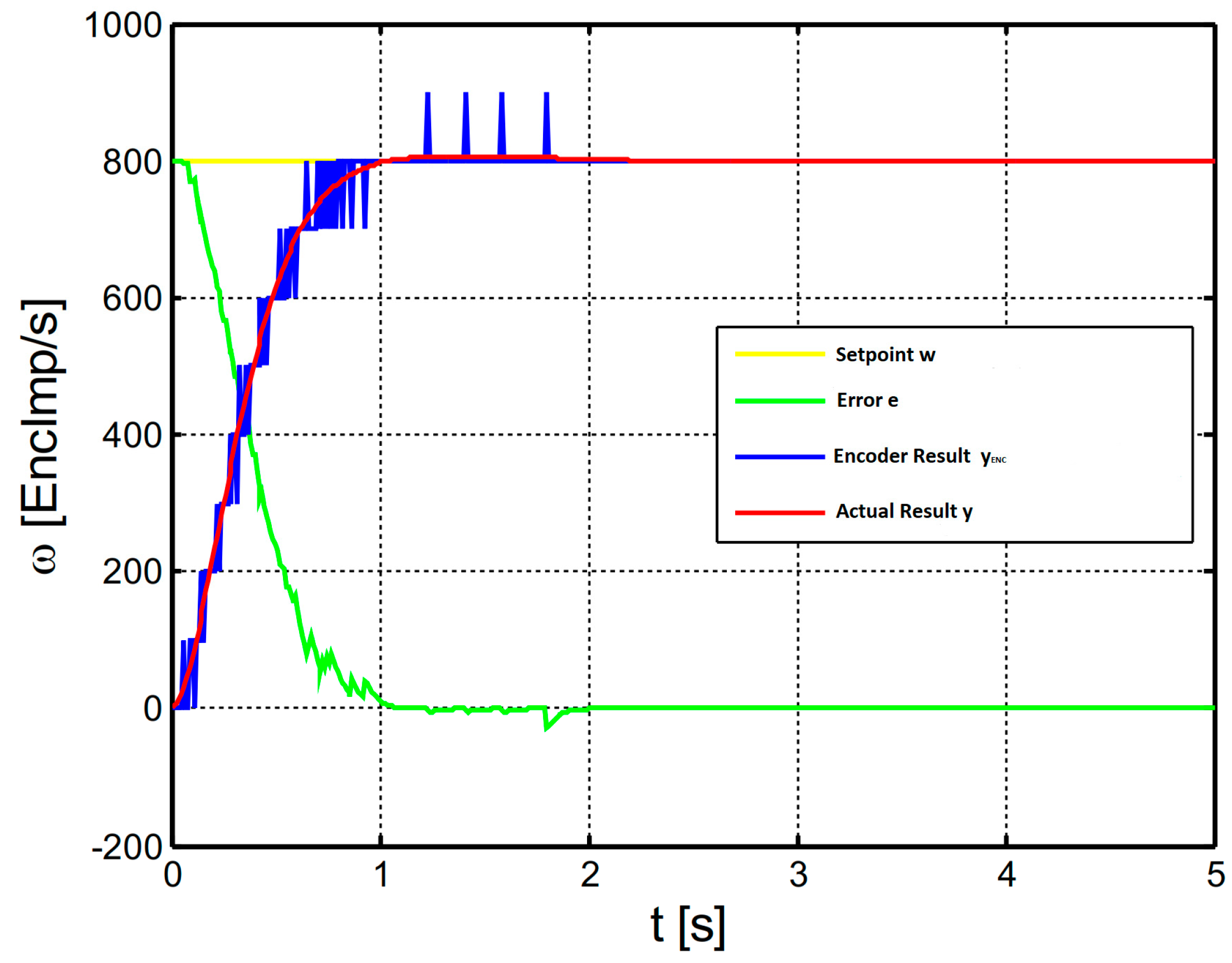
The permanent oscillation is so small that it can no longer be seen in the diagram. The system reached the end value after approximately one second. The controller is thus set almost ideally. Finally, the manipulated variable-limited and quantized control loop was modeled with Simulink and given the same step response. The result can be seen in Figure 8. It can be seen that the actual y value has reached the setpoint u after approx. one second. Furthermore, as expected, a slight overshoot of the actual value and a strong quantization of the speed by the rotary encoder can be seen. Overall, however, this is a very satisfactory result.

Figure 8.
Simulation result of the speed controller.
4. Results and Discussion
The result section deals with some test scenarios with which the quality of the parameterized robot can be determined. For this purpose, relevant data were recorded by the robot and then displayed graphically. The data were recorded directly from the microcontroller for the experiments where only the drive speed is shown. The data source was therefore recorded lucidly. In the trajectory experiments, only the mini computer was recorded. However, its sampling rate is not synchronized with the robot, so a small amount of jitter can occur in the sampled values. It is sometimes reflected in small jumps in the curves. Table 2 contains the significant parameters for the experiment environment, which shows the obstacle type, i.e., static, and the number of static obstacles is eight and 4 × 4 feet in size.
Table 2.
Significant experimental parameters.
4.1. Speed Control Loop
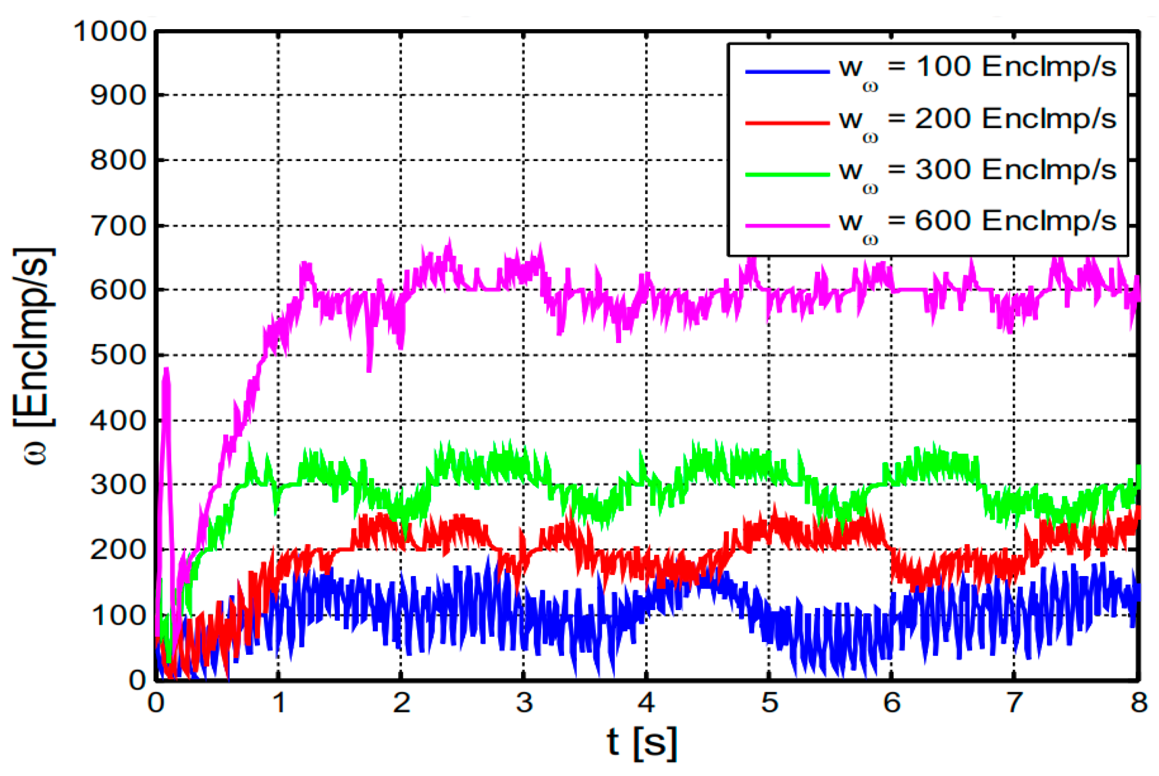
The first experiment analyzed the speed controller. The quantization of the actual speed created by the rotary encoder was 100 EncImp/s. Step responses of the velocity loop from a standing start were recorded for velocities of 100, 200, 300 and 600 EncImp/s. Based on the simulations already carried out on the ideal robot model, the final value should be reached after about one second. The step responses were recorded in the hallway of the electrical engineering (EE) building at the University of King Abdulaziz. Since the ground there is very flat, it is an almost interference-free environment. Figure 9 shows the four-step responses in a jitter-free time diagram, where the graphs were previously smoothed with a digital PT1 element with a time constant of 20 ms.
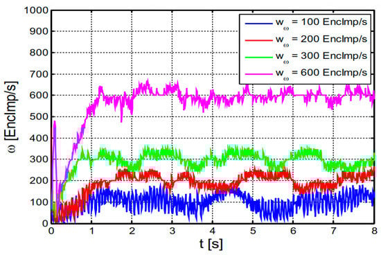
Figure 9.
Different step responses of the closed speed controller.
It is easy to see that all step responses reached the final value after about a second and then oscillated around it. The deviation of the slightly smoothed measured values was around ±50 EncImp/s for each graph. This is a very good value. The oscillating behavior probably resulted from many individual components.
First, the controlled system, i.e., the drive train, is very complex since it combines many mass-spring-damper systems and some non-linearities. For the sake of simplicity, however, the track was modeled as a PT2 system. The effect of the play can be seen very well in the magenta graph. The speed jumps to a very high value for a short time in the beginning. This results from the no-load acceleration of the transmission during play. If it is used up, the motors are abruptly braked, and the robot accelerates as desired.
4.2. Step Response
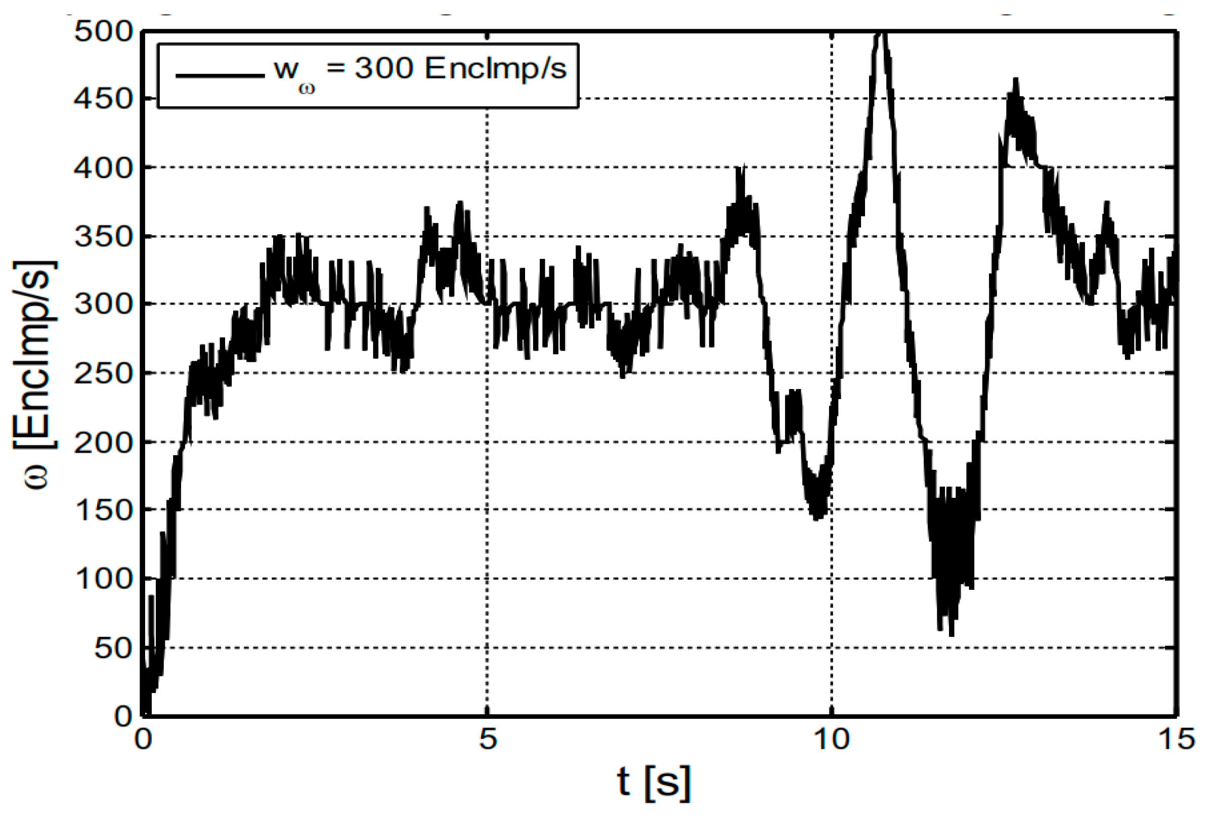
On the other hand, the system also oscillated due to the rotary encoder’s quantization and the controller’s setting. It was parameterized intentionally, so it tends to oscillate, but the amplitude remained below the encoder resolution. A step response followed with a speed of 300 EncImp/s. This was carried out in the courtyard of the EE building of the University of King Abdulaziz. The ground there has bumps at periodic intervals, representing a strong disturbance for the slow drive speed. The bumps are small valleys on the ground surface. The recording is shown in Figure 10 and contains measured values smoothed with a PT1 element with a time constant of 20 ms.
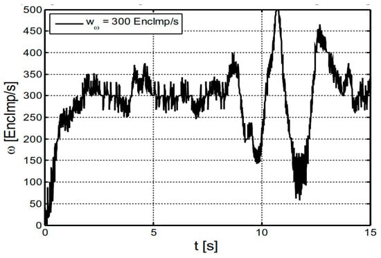
Figure 10.
Step response of closed speed controller with disturbance.
The graph shows that the controller regulated the robot quite well. It should be noted that the quantization of the encoder was 100 EncImp/s steps. Without a fault, the controller deviated from the setpoint here by −50/+75 EncImp/s. After around eight seconds, the speed increased slightly as the robot’s front wheels sank into the bump. The robot actively tried to slow down the increase in speed using the motors. Now the wheels had to be lifted out of the valley again. This required a lot of energy, which first had to be made available by the drive. However, since it was very slow due to the last braking, it took some time for the motors to build up enough power again. This can be seen in the graph by the valley just before the ten-second mark. After overcoming the first obstacle, the robot accelerated strongly due to the still very large manipulated variable and the speed overshoots. Finally, the procedure started again since the rear wheels sank into the bump. However, the braking effect was much greater here since most of the robot’s weight was on the rear axle.
On the whole, however, the disturbance was quite well-compensated for. It must be remembered that this is a violent and short-term disruption. The disturbance would be completely corrected if the robot were to work on a long uphill or downhill gradient. It should also be noted here that the cruise control is also active at zero speed, i.e., when stationary. This means that the robot is actively braking with its motors. If one tries to move the robot with an external force, this is quite easy at first, but it becomes more and more difficult as the robot defends itself against this disturbance more and more.
4.3. Avoiding Obstacles
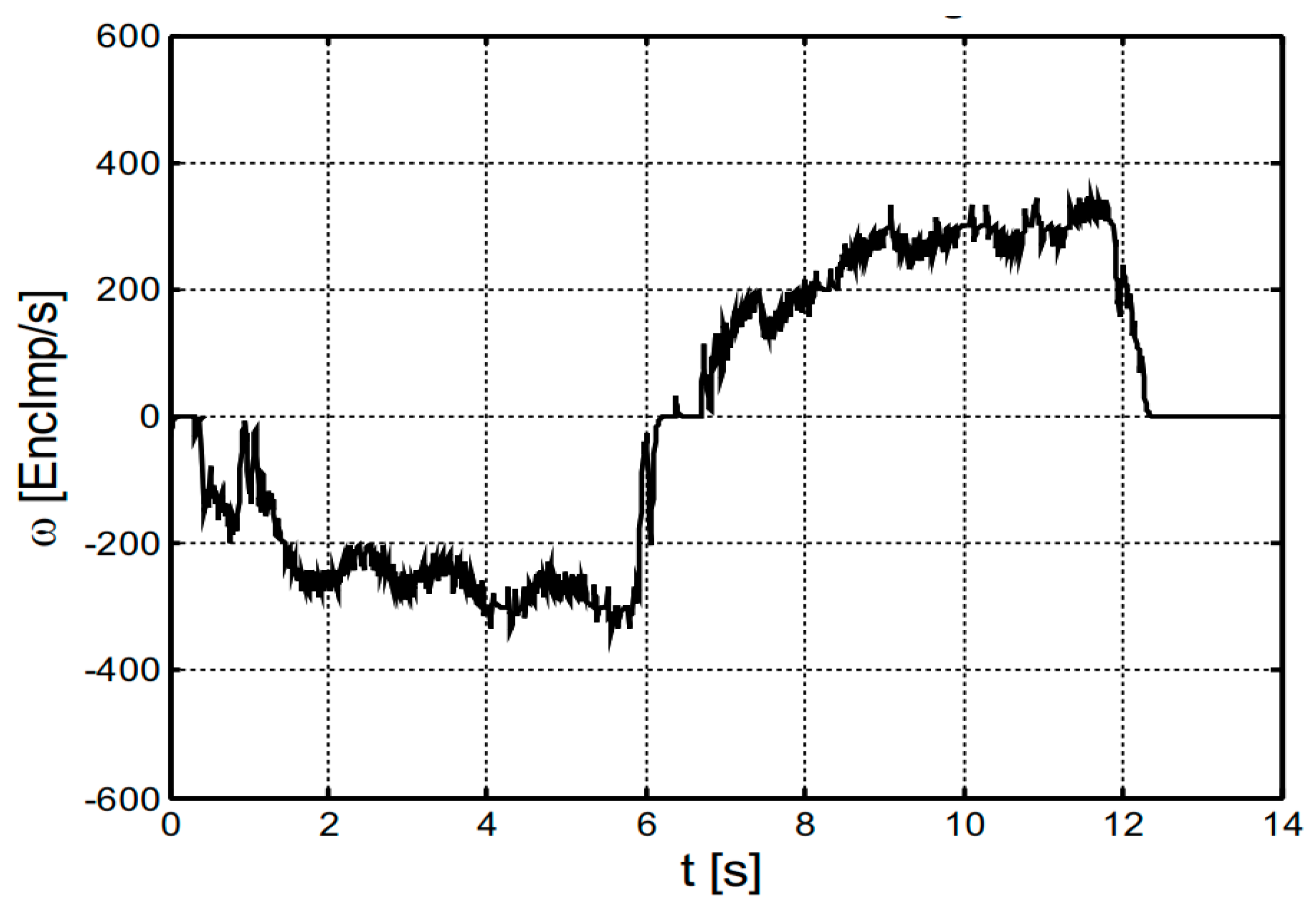
Now, the course of the speed when driving around an obstacle is shown for completeness. The robot should move backwards for 6 s with 300 EncImp/s and then forward at the same speed for 6s. The course of the actual speed, which was smoothed with a PT1 element with a time constant of 20 ms, is shown in Figure 11.
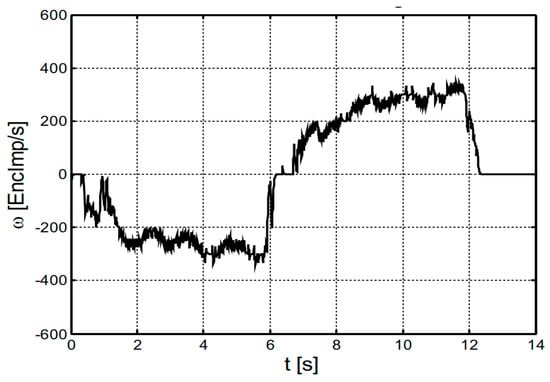
Figure 11.
Speed curve when avoiding an obstacle.
A good approximation of the setpoint can be seen for both setpoint jumps. Thus, the robot moved fast enough to avoid an obstacle.
Different categories of healthcare-based telepresence robots have been discussed [48,49,50,51,52,53,54]. Different telepresence robots used by healthcare doctors to interact with patients during their initial visit have been described. The major advantage of the proposed technique is to help frontline healthcare workers to be safe from an infected patient.
Most of the proposed controlling techniques can interact with telepresence robots efficiently and robustly, except for the lack of control in the scenario of disconnection or delays. Based on the review, all existing telepresence robots cannot behave intelligently according to the controller behavior in communication issues. This study shows better, more effective and more efficient control techniques for interacting with telepresence robots for specific purposes or in general. It also shows the lacking features of existing telepresence robots, i.e., modification of design and lack of human interaction, (e.g., chaotic behavior of telepresence robots in case of delays or connectivity issues). Second, it shows the object avoidance capability and addition of peripheral attachments for more human-like behavior in a remote environment. A focus on development will help researchers.
4.4. Self-Localization
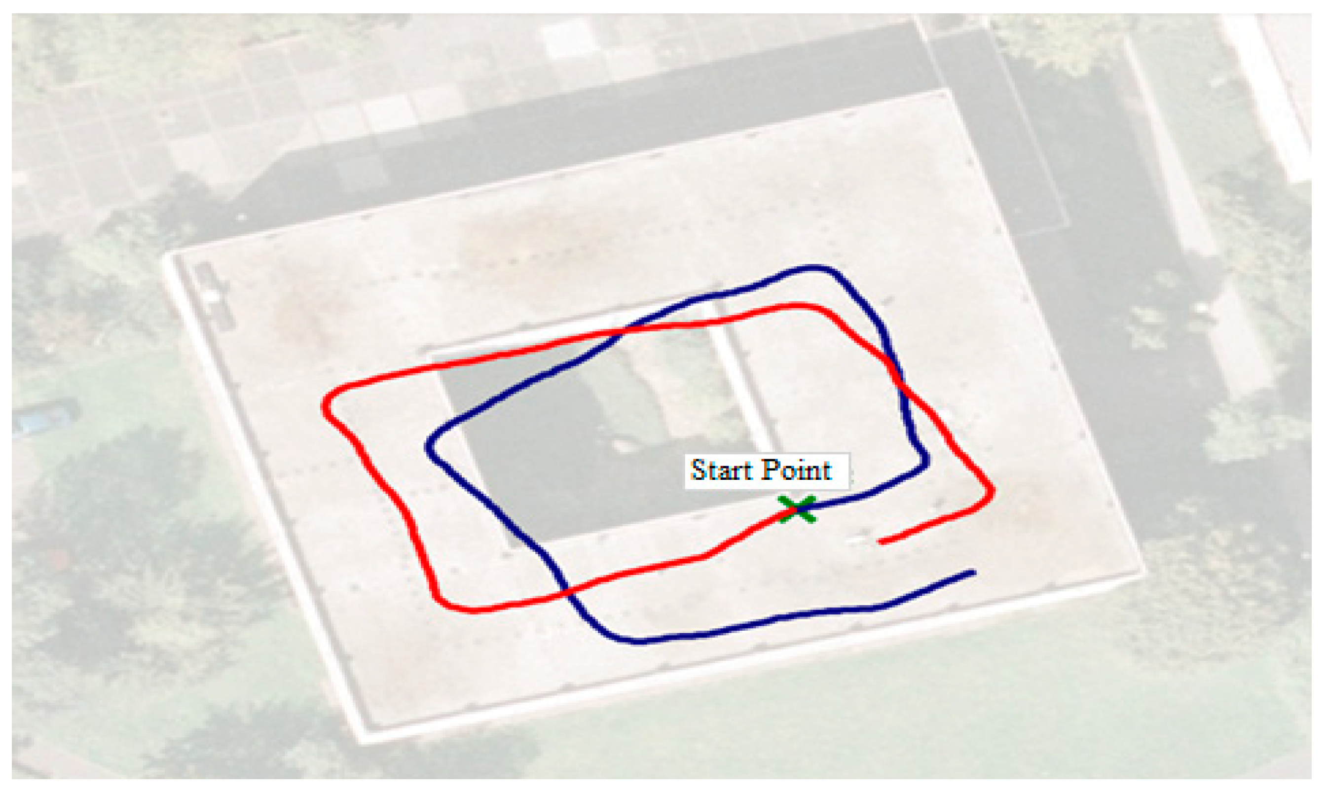
This section describes a simple but impressive test. Using the magnetometer [56], the robot was driven in manual mode twice in a circle across the corridor of the EE building of the University of King Abdulaziz.
One tour was driven clockwise, and one counter-clockwise. The position was recorded, and the resulting trajectories were finally superimposed on a Google Maps aerial photograph. The size of the trajectories was subsequently adjusted so that they fit reasonably into the building. However, the aspect ratio and orientation have been retained. The result can be seen in Figure 12.
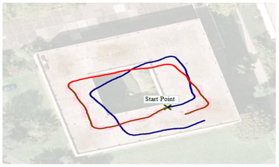
Figure 12.
Self-estimates of robot position. Blue track was travelled counter-clockwise and red track was travelled clockwise.
The red trajectory, which runs clockwise, was recorded first. It can be seen that the calibration of the magnetometer was very good. The start and end points of the trajectory are the same. In the image, however, these points are slightly apart. Each control cycle adds a correction value to the old position, so the position is an incremental value. This, of course, leads to error accumulation so that the estimated position deviates more and more from the actual position as the distance increases. On the first three straight lines of the red track, one can see that the tracks run fairly parallel to the outline of the building. This angle is no longer so accurate in the fourth straight line, so the error has probably increased the most here. On the other hand, one looks at the blue track, which was travelled counter-clockwise, the second straight section is parallel to the outline of the building. However, the other straight sections then deviate.
The strong angle errors in the trajectories can have many causes. On the one hand, the magnetometer calibration can be insufficient since it may have been held at an angle during calibration, rotated too quickly, or had interference fields. On the other hand, many sources of interference in the building generate magnetic fields or deform the earth’s magnetic field. Power lines, heating systems and stair railings are examples of this. Drifting of the magnetometer cannot be ruled out either. Online calibration would help here.
4.5. Complex Path
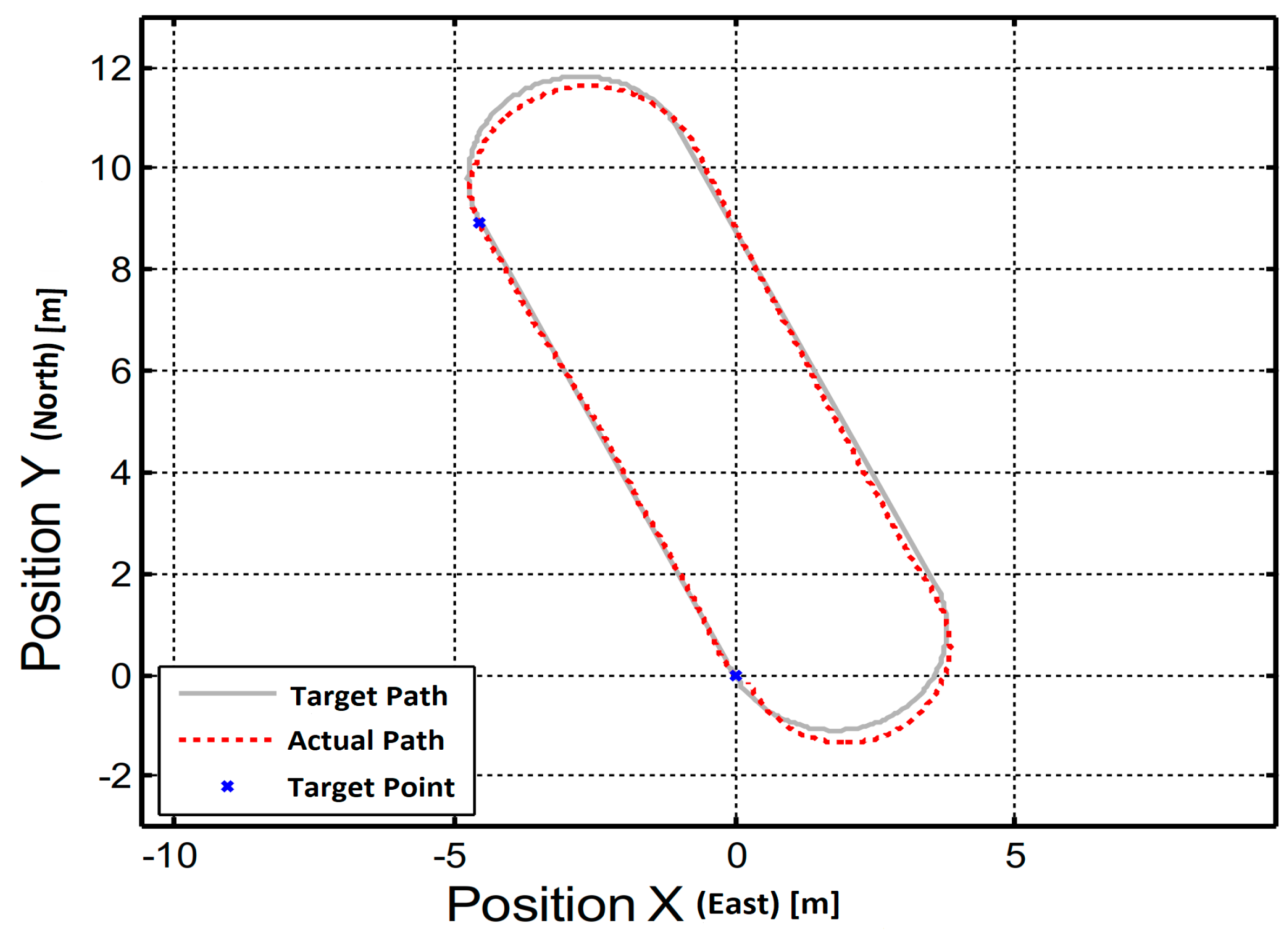
The last test shows how well the robot can travel a more complex path. This test was also carried out in the courtyard of the university campus. The robot had to drive straight ahead for 10 m and then return to its original point, but in doing so, it had to approximately assume the original orientation. The path definition is given in Table 3.
Table 3.
Lane definition.
Figure 13 now shows the target path and the actual path. The actual path consists of the coordinates measured by the robot. In the ideal case, it should therefore correspond to the target path. However, the actual path does not describe the path travelled, as this cannot be determined without special measuring devices. In addition, the marked target points are marked.
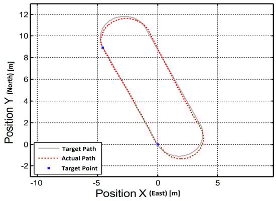
Figure 13.
Calculated and driven trajectories.
It can be seen that the target path was maintained quite well. There was only a small deviation in the orbits. This is mainly because, in point 1, the second path section was calculated from the current robot position. However, this did not correspond one hundred percent to the desired position. This resulted in a deviation from the previously calculated path. However, the targets were reached very well.
It must be noted that the robot did not return exactly to the starting point during this journey. It was about 2 m away from it. However, this is due to the inaccuracy of the self-localization. The orientation, on the other hand, was correct. Auto-MERLIN is a highly nonlinear system having a gearbox for power transmission, and it is not easy to obtain its accurate mathematical model. Therefore, a system identification approach was used to find the approximate model of the system. The root locus method was used to design a speed controller by introducing appropriate poles and zeros shown in Figure 6. The results validate the identified model of the system. The experimental data are given in the form of Table 4.
Table 4.
Experimental data for different trials.
5. Conclusions
A control board and a voltage regulator for the steering servo motor are also required to maneuver the robot successfully. Fundamentally different models were successfully developed, built and tested. A new motor mount had to be created for the drive, to which two motors could be attached. It was necessary because the existing motor alone could not generate enough torque to move to and maintain the robot’s stable operating points. In addition, the brackets for the ten distance sensors had to be designed.
In the proposed research work, we designed speed and position control. The speed control loop was designed using the PID controller. An algorithm was developed for the state machine to avoid obstacles. It was a complex task that needed precise analysis and design. In the case of the robot, the high-level controller was a mini-computer running the application program. To this end, controlled test drives were undertaken, and the results were evaluated. Finally, the ideally adjusted robot was checked for its desired behavior.
The robot was tested over the step responses and the self-localization to test the maneuverability and control. It was seen from the results that the robot followed the given path with an ignorable number of hits. The robot’s calculated driven trajectory was measured and provided very precise results. It can be seen that the target path was maintained quite well.
As the summary suggests, software drivers should be written for the hardware. The timing of these drivers probably needs to be adjusted. So far, no driver has been developed for the SD card. This development would likely also fill a separate research task. In addition, the soldering pads on the control board used are attached the wrong way around so that the SD card slot cannot be attached. There is also no driver for the real-time clock. Another problem, which became apparent in the course of the research, is the correct self-localization of the robot. So far, it estimates its position by gradually adding up the distance travelled in the direction of orientation. First, the arc length travelled is used as the tangent length of the motion vector. It is also tolerable for small changes in direction. However, the systematic error accumulates over time when cornering. A correct solution to this problem would be quite complex and likely bring little improvement.
Author Contributions
Conceptualization, A.A. and A.S.; methodology, M.N.K.; software, M.N.K.; validation, A.A., A.S. and M.N.K.; formal analysis, M.N.K.; investigation, A.S.; resources, A.S.; writing—original draft preparation, M.N.K.; writing—review and editing, A.S.; supervision, M.N.K.; funding acquisition, A.A. All authors have read and agreed to the published version of the manuscript.
Funding
The authors extend their appreciation to the Deputyship for Research and Innovation, the Ministry of Education in Saudi Arabia for funding this research work through the project number IF2/PSAU/2022/01/22378.
Institutional Review Board Statement
Not applicable.
Informed Consent Statement
Not applicable.
Data Availability Statement
Not applicable.
Acknowledgments
The authors acknowledge the support of the Ministry of Education in Saudi Arabia, and Faculty of Computing and Information Technology, King Abdulaziz University, Jeddah 21589, Saudi Arabia.
Conflicts of Interest
The authors declare no conflict of interest.
References
- Zhou, X.; Xu, P.; Lee, F.C. A Novel Current-Sharing Control Technique for Low-Voltage High-Current Voltage Regulator Module Applications. IEEE Trans. Power Electron. 2000, 15, 1153–1162. [Google Scholar] [CrossRef]
- Gil, A.; Segura, J.; Temme, N.M. Numerical Methods for Special Functions; SIAM: Philadelphia, PE, USA, 2007; ISBN 0-89871-634-9. [Google Scholar]
- Guillén-Climent, S.; Garzo, A.; Muñoz-Alcaraz, M.N.; Casado-Adam, P.; Arcas-Ruiz-Ruano, J.; Mejías-Ruiz, M.; Mayordomo-Riera, F.J. A Usability Study in Patients with Stroke Using MERLIN, a Robotic System Based on Serious Plays for Upper Limb Rehabilitation in the Home Setting. J. Neuroeng. Rehabil. 2021, 18, 41. [Google Scholar] [CrossRef] [PubMed]
- Karimi, M.; Roncoli, C.; Alecsandru, C.; Papageorgiou, M. Cooperative Merging Control via Trajectory Optimization in Mixed Vehicular Traffic. Transp. Res. Part C Emerg. Technol. 2020, 116, 102663. [Google Scholar] [CrossRef]
- Kitazawa, O.; Kikuchi, T.; Nakashima, M.; Tomita, Y.; Kosugi, H.; Kaneko, T. Development of Power Control Unit for Compact-Class Vehicle. SAE Int. J. Altern. Powertrains 2016, 5, 278–285. [Google Scholar] [CrossRef]
- Rodríguez-Lera, F.J.; Matellán-Olivera, V.; Conde-González, M.Á.; Martín-Rico, F. HiMoP: A Three-Component Architecture to Create More Human-Acceptable Social-Assistive Robots. Cogn. Process. 2018, 19, 233–244. [Google Scholar] [CrossRef]
- Narayan, P.; Wu, P.; Campbell, D.; Walker, R. An Intelligent Control Architecture for Unmanned Aerial Systems (UAS) in the National Airspace System (NAS). In Proceedings of the AIAC12: 2nd Australasian Unmanned Air Vehicles Conference; Waldron Smith Management: Melbourne, Australia, 2007; pp. 1–12. [Google Scholar]
- Laengle, T.; Lueth, T.C.; Rembold, U.; Woern, H. A Distributed Control Architecture for Autonomous Mobile Robots-Implementation of the Karlsruhe Multi-Agent Robot Architecture (KAMARA). Adv. Robot. 1997, 12, 411–431. [Google Scholar] [CrossRef]
- de Oliveira, R.W.; Bauchspiess, R.; Porto, L.H.; de Brito, C.G.; Figueredo, L.F.; Borges, G.A.; Ramos, G.N. A Robot Architecture for Outdoor Competitions. J. Intell. Robot. Syst. 2020, 99, 629–646. [Google Scholar] [CrossRef]
- Atsuzawa, K.; Nilwong, S.; Hossain, D.; Kaneko, S.; Capi, G. Robot Navigation in Outdoor Environments Using Odometry and Convolutional Neural Network. In Proceedings of the IEEJ International Workshop on Sensing, Actuation, Motion Control, and Optimization (SAMCON), Chiba, Japan, 4–6 March 2019. [Google Scholar]
- Cuesta, F.; Ollero, A.; Arrue, B.C.; Braunstingl, R. Intelligent Control of Nonholonomic Mobile Robots with Fuzzy Perception. Fuzzy Sets Syst. 2003, 134, 47–64. [Google Scholar] [CrossRef]
- Ahmadzadeh, A.; Jadbabaie, A.; Kumar, V.; Pappas, G.J. Multi-UAV Cooperative Surveillance with Spatio-Temporal Specifications. In Proceedings of the 45th IEEE Conference on Decision and Control, IEEE, San Diego, CA, USA, 13–15 December 2006; pp. 5293–5298. [Google Scholar]
- Anavatti, S.G.; Francis, S.L.; Garratt, M. Path-Planning Modules for Autonomous Vehicles: Current Status and Challenges. In Proceedings of the 2015 International Conference on Advanced Mechatronics, Intelligent Manufacture, and Industrial Automation (ICAMIMIA), IEEE, Surabaya, Indonesia, 15–17 October 2015; pp. 205–214. [Google Scholar]
- Alami, R.; Chatila, R.; Fleury, S.; Ghallab, M.; Ingrand, F. An Architecture for Autonomy. Int. J. Robot. Res. 1998, 17, 315–337. [Google Scholar] [CrossRef]
- Microchip Technology Inc.—DSPIC33FJ32MC302-I/SO—16-Bit DSC, 28LD,32KB Flash, Motor, DMA,40 MIPS, NanoWatt—Allied Electronics & Automation, Part of RS Group. Available online: https://www.alliedelec.com/product/microchip-technology-inc-/dspic33fj32mc302-i-so/70047032/?gclid=Cj0KCQiA1ZGcBhCoARIsAGQ0kkqp_8dGIbQH-bCsv1_OMKGCqwJWGl9an18jsfWWs9DhtuKKYZec_aoaAheKEALw_wcB&gclsrc=aw.ds (accessed on 28 November 2022).
- #835 RTR Savage 25. Available online: https://www.hpiracing.com/en/kit/835 (accessed on 28 November 2022).
- Hitec HS-5745MG Servo Specifications and Reviews. Available online: https://servodatabase.com/servo/hitec/hs-5745mg (accessed on 28 November 2022).
- Optical Encoder M101|MEGATRON. Available online: https://www.megatron.de/en/products/optical-encoders/optoelectronic-encoder-m101.html (accessed on 28 November 2022).
- Milla, K.; Kish, S. A Low-Cost Microprocessor and Infrared Sensor System for Automating Water Infiltration Measurements. Comput. Electron. Agric. 2006, 53, 122–129. [Google Scholar] [CrossRef]
- Estlin, T.A.; Volpe, R.; Nesnas, I.; Mutz, D.; Fisher, F.; Engelhardt, B.; Chien, S. Decision-Making in a Robotic Architecture for Autonomy; California Institute of Technology: Pasadena, CA, USA, 2001. [Google Scholar]
- Kress, R.L.; Hamel, W.R.; Murray, P.; Bills, K. Control Strategies for Teleoperated Internet Assembly. IEEE/ASME Trans. Mechatron. 2001, 6, 410–416. [Google Scholar] [CrossRef]
- Goldberg, K.; Siegwart, R. Beyond Webcams: An Introduction to Online Robots; MIT Press: Cambridge, MA, USA, 2002; ISBN 0-262-07225-4. [Google Scholar]
- De Brito, C.G. Desenvolvimento de Um Sistema de Localização Para Robôs Móveis Baseado Em Filtragem Bayesiana Não-Linear. Undergraduate Thesis, Universidade de Bras’ılia, Brasilia, Brazil, 2018. [Google Scholar]
- Rozevink, S.G.; van der Sluis, C.K.; Garzo, A.; Keller, T.; Hijmans, J.M. HoMEcare ARm RehabiLItatioN (MERLIN): Telerehabilitation Using an Unactuated Device Based on Serious Plays Improves the Upper Limb Function in Chronic Stroke. J. NeuroEngineering Rehabil. 2021, 18, 48. [Google Scholar] [CrossRef] [PubMed]
- Schilling, K. Tele-Maintenance of Industrial Transport Robots. IFAC Proc. Vol. 2002, 35, 139–142. [Google Scholar] [CrossRef]
- Garzo, A.; Arcas-Ruiz-Ruano, J.; Dorronsoro, I.; Gaminde, G.; Jung, J.H.; Téllez, J.; Keller, T. MERLIN: Upper-Limb Rehabilitation Robot System for Home Environment. In Proceedings of the International Conference on NeuroRehabilitation; Springer: Berlin/Heidelberg, Germany, 2020; pp. 823–827. [Google Scholar]
- Ahmad, A.; Babar, M.A. Software Architectures for Robotic Systems: A Systematic Mapping Study. J. Syst. Softw. 2016, 122, 16–39. [Google Scholar] [CrossRef]
- Sharma, O.; Sahoo, N.C.; Puhan, N.B. Recent Advances in Motion and Behavior Planning Techniques for Software Architecture of Autonomous Vehicles: A State-of-the-Art Survey. Eng. Appl. Artif. Intell. 2021, 101, 104211. [Google Scholar] [CrossRef]
- Ziegler, J.; Werling, M.; Schroder, J. Navigating Car-like Robots in Unstructured Environments Using an Obstacle Sensitive Cost Function. In Proceedings of the 2008 IEEE Intelligent Vehicles Symposium, IEEE, Eindhoven, The Netherlands, 4–6 June 2008; pp. 787–791. [Google Scholar]
- González-Santamarta, M.Á.; Rodríguez-Lera, F.J.; Álvarez-Aparicio, C.; Guerrero-Higueras, Á.M.; Fernández-Llamas, C. MERLIN a Cognitive Architecture for Service Robots. Appl. Sci. 2020, 10, 5989. [Google Scholar] [CrossRef]
- Shao, J.; Xie, G.; Yu, J.; Wang, L. Leader-Following Formation Control of Multiple Mobile Robots. In Proceedings of the 2005 IEEE International Symposium on, Mediterrean Conference on Control and Automation Intelligent Control, Limassol, Cyprus, 27–29 June 2005; pp. 808–813. [Google Scholar]
- Faisal, M.; Hedjar, R.; Al Sulaiman, M.; Al-Mutib, K. Fuzzy Logic Navigation and Obstacle Avoidance by a Mobile Robot in an Unknown Dynamic Environment. Int. J. Adv. Robot. Syst. 2013, 10, 37. [Google Scholar] [CrossRef]
- Favarò, F.; Eurich, S.; Nader, N. Autonomous Vehicles’ Disengagements: Trends, Triggers, and Regulatory Limitations. Accid. Anal. Prev. 2018, 110, 136–148. [Google Scholar] [CrossRef]
- Gopalswamy, S.; Rathinam, S. Infrastructure Enabled Autonomy: A Distributed Intelligence Architecture for Autonomous Vehicles. In Proceedings of the 2018 IEEE Intelligent Vehicles Symposium (IV), Changshu, China, 26–30 June 2018; pp. 986–992. [Google Scholar]
- Allen, J.F. Towards a General Theory of Action and Time. Artif. Intell. 1984, 23, 123–154. [Google Scholar] [CrossRef]
- Hu, H.; Brady, J.M.; Grothusen, J.; Li, F.; Probert, P.J. LICAs: A Modular Architecture for Intelligent Control of Mobile Robots. In Proceedings of the 1995 IEEE/RSJ International Conference on Intelligent Robots and Systems. Human Robot Interaction and Cooperative Robots, Pittsburgh, PA, USA, 5–9 August 1995; Volume 1, pp. 471–476. [Google Scholar]
- Alami, R.; Chatila, R.; Espiau, B. Designing an Intelligent Control Architecture for Autonomous Robots. In Proceedings of the ICAR, Tokyo, Japan, November 1993; Volume 93, pp. 435–440. [Google Scholar]
- Khan, M.N.; Hasnain, S.K.; Jamil, M.; Imran, A. Electronic Signals and Systems: Analysis, Design and Applications; River Publishers: Gistrup, Denmark, 2022. [Google Scholar]
- Kang, J.-M.; Chun, C.-J.; Kim, I.-M.; Kim, D.I. Channel Tracking for Wireless Energy Transfer: A Deep Recurrent Neural Network Approach. arXiv 2018, arXiv:1812.02986. [Google Scholar]
- Zhao, W.; Gao, Y.; Ji, T.; Wan, X.; Ye, F.; Bai, G. Deep Temporal Convolutional Networks for Short-Term Traffic Flow Forecasting. IEEE Access 2019, 7, 114496–114507. [Google Scholar] [CrossRef]
- Schilling, K.J.; Vernet, M.P. Remotely Controlled Experiments with Mobile Robots. In Proceedings of the Thirty-Fourth Southeastern Symposium on System Theory (Cat. No. 02EX540), Huntsville, AL, USA, 19 March 2002; pp. 71–74. [Google Scholar]
- Moon, T.-K.; Kuc, T.-Y. An Integrated Intelligent Control Architecture for Mobile Robot Navigation within Sensor Network Environment. In Proceedings of the 2004 IEEE/RSJ International Conference on Intelligent Robots and Systems (IROS) (IEEE Cat. No. 04CH37566), Sendai, Japan, 28 September–2 October 2004; Volume 1, pp. 565–570. [Google Scholar]
- Lefèvre, S.; Vasquez, D.; Laugier, C. A Survey on Motion Prediction and Risk Assessment for Intelligent Vehicles. Robomech. J. 2014, 1, 1. [Google Scholar] [CrossRef]
- Behere, S.; Törngren, M. A Functional Architecture for Autonomous Driving. In Proceedings of the First International Workshop on Automotive Software Architecture, Montreal, QC, Canada, 4 May 2015; pp. 3–10. [Google Scholar]
- Carvalho, A.; Lefévre, S.; Schildbach, G.; Kong, J.; Borrelli, F. Automated Driving: The Role of Forecasts and Uncertainty—A Control Perspective. Eur. J. Control 2015, 24, 14–32. [Google Scholar] [CrossRef]
- Liu, P.; Paden, B.; Ozguner, U. Model Predictive Trajectory Optimization and Tracking for On-Road Autonomous Vehicles. In Proceedings of the 2018 21st International Conference on Intelligent Transportation Systems (ITSC), Miami, FL, USA, 4–7 November 2018; pp. 3692–3697. [Google Scholar]
- Weiskircher, T.; Wang, Q.; Ayalew, B. Predictive Guidance and Control Framework for (Semi-) Autonomous Vehicles in Public Traffic. IEEE Trans. Control Syst. Technol. 2017, 25, 2034–2046. [Google Scholar] [CrossRef]
- Zhu, H.; Brito, B.; Alonso-Mora, J. Decentralized probabilistic multi-robot collision avoidance using buffered uncertainty-aware Voronoi cells. Auton. Robot. 2022, 46, 401–420. [Google Scholar] [CrossRef]
- Batmaz, A.U.; Maiero, J.; Kruijff, E.; Riecke, B.E.; Neustaedter, C.; Stuerzlinger, W. How automatic speed control based on distance affects user behaviours in telepresence robot navigation within dense conference-like environments. PLoS ONE 2020, 15, e0242078. [Google Scholar] [CrossRef]
- Xia, P.; McSweeney, K.; Wen, F.; Song, Z.; Krieg, M.; Li, S.; Du, E.J. Virtual Telepresence for the Future of ROV Teleoperations: Opportunities and Challenges. In Proceedings of the SNAME 27th Offshore Symposium, Houston, TX, USA, 22 February 2022. [Google Scholar]
- Dong, Y.; Pei, M.; Zhang, L.; Xu, B.; Wu, Y.; Jia, Y. Stitching videos from a fisheye lens camera and a wide-angle lens camera for telepresence robots. Int. J. Soc. Robot. 2022, 14, 733–745. [Google Scholar] [CrossRef]
- Correia, D.; Silva, M.F.; Moreira, A.P. A Survey of high-level teleoperation, monitoring and task assignment to Autonomous Mobile Robots. In Proceedings of the 2022 IEEE International Conference on Autonomous Robot Systems and Competitions (ICARSC), Santa Maria da Feira, Portugal, 29–30 April 2022; pp. 218–225. [Google Scholar]
- Xin, J.; Zhong, J.; Yang, F.; Cui, Y.; Sheng, J. An improved genetic algorithm for path-planning of unmanned surface vehicle. Sensors 2019, 19, 2640. [Google Scholar] [CrossRef] [PubMed]
- Wang, Z.; Fang, J.; Dai, X.; Zhang, H.; Vlacic, L. Intelligent vehicle self-localization based on double-layer features and multilayer LIDAR. IEEE Trans. Intell. Veh. 2020, 5, 616–625. [Google Scholar] [CrossRef]
- Chen, D.; Weng, J.; Huang, F.; Zhou, J.; Mao, Y.; Liu, X. Heuristic monte carlo algorithm for unmanned ground vehicles realtime localization and mapping. IEEE Trans. Veh. Technol. 2020, 69, 10642–10655. [Google Scholar] [CrossRef]
- Types of Magnetometers—Technical Articles. Available online: https://www.allaboutcircuits.com/technical-articles/types-of-magnetometers/ (accessed on 28 November 2022).

Disclaimer/Publisher’s Note: The statements, opinions and data contained in all publications are solely those of the individual author(s) and contributor(s) and not of MDPI and/or the editor(s). MDPI and/or the editor(s) disclaim responsibility for any injury to people or property resulting from any ideas, methods, instructions or products referred to in the content. |
© 2023 by the authors. Licensee MDPI, Basel, Switzerland. This article is an open access article distributed under the terms and conditions of the Creative Commons Attribution (CC BY) license (https://creativecommons.org/licenses/by/4.0/).