Dynamic Characteristics Analysis of an Assembly Robot for a Wine Box Base Considering Radial and Axial Clearances in a 3D Revolute Joint

Abstract

Precisely fitting the bottom sticker of the wine box base to the base model with glue is an important process of the wine box base production line. The influence of joint clearance in the assembly robot on the assembly precision of wine box bases is investigated. We analyze the axial clearance and radial clearance in a 3D revolute joint of the assembly robot and present 12 possible contact forms between bearings and journals, as well as three modes of free flight mode, continuous contact mode, and pseudo penetration mode between them under the different contact forms. The contact force models of normal and tangential force between bearings and journals are established using the Lankarani–Nikravesh contact model and modified Coulomb friction law, respectively. Taking the joint clearance of one joint of the wine box base assembly robot as an example, the dynamic equations of the joint with clearance are established, and the dynamic characteristics of the robot caused by the joint clearance are analyzed. The results show that, the larger the clearance, the more easily the dynamic characteristics of the robot end effector are influenced.

1. Introduction

One of the important processes of the wine box base production line involves precisely fitting the bottom sticker of the wine box base to the base model with glue, and its fitting accuracy directly affects the quality of the wine box [1]. The working accuracy, repeatability, and stability of the assembly robot installed on the wine box base production line are the keys to ensuring the fitting accuracy. The working precision, repeatability, and stability of the assembly robot directly determine the rate of defective products in the production line [2,3,4]. However, owing to manufacturing errors, assembly errors, mechanical wear, and other reasons, the joints of the assembly robot have different degrees of joint clearances. Joint clearance is an inevitable nonlinear factor that affects the fitting accuracy of the robot [5].

In the past decades, scholars have studied joint clearance through different methods. Flores et al. [6,7,8] took the four-link mechanism as the target of investigation, studied the joint clearance of one spherical joint, modeled the spherical joint based on Cartesian coordinates, and established the contact force model.

On the basis of the numerical results of finite element analysis, Liu et al. [9] scrutinized the cylindrical joint with clearance. Through proper assumptions and analysis of the contact area, force distribution, and maximum effective shipment, a homologous model was proposed to more effectively analyse the dynamic feature of the cylindrical joint with clearance. Zhang et al. [10,11] deduced the theory of reducing the influence of revolute joint clearance based on the redundant driving mechanism. Based on this method, the kinematics and dynamics of the planar 4-RRR mechanism were analyzed. The constraint mechanisms of ideal joints and joints with clearance were compared through the two-step Bathe integration method. The experiment proved that the redundant driving mechanism can effectively control the size of joint clearance.

Erkaya et al. [12] analyzed the direct impact of the clearance of the revolute joint on the motion feature and dynamic performance of the end effect of the welding robot. Zhao et al. [13] studied a lubrication model for the collision of joint clearance on system dynamics. Then, the lubrication model was solved by ANSYS software and the average Reynolds equation was introduced into the system dynamics equation. The dynamic performance of the planar mechanism with clearance was analyzed, which proved that the impact of joint clearance on the mechanism dynamics could be reduced through the lubrication model.

Xiang et al. [14] used an interval algorithm and introduced Chebyshev polynomials to derive the kinematic equations of the impact of nonlinear external forces on the mechanism; analyzed the dynamics of the space mechanism when the parameters were uncertain; and quantified the changes in uncertain parameters, which was helpful to derive the law of the motion of the end effectors of space robots.

According to the clearance of the revolute joint, Filipe Marques [15,16] deduced a formula that can simulate the joint clearance and analyzed the kinematic performance of a classic mechanism including clearance according to the Newton Euler method. Zhao [17] proposed a calculation method for the clearance of the revolute joint. Taking the spacecraft body and two flexible links of the space robot as the research object, the effect of joint clearance on the precision of the end effector of the space robot is predicted using the system dynamics equation. Zhang [18] studied the revolute joint with radial clearance. The joint belongs to a revolute pair in the planar 3-RRR mechanism. By establishing the root mean square error (RMSE) of angular velocity and taking the RMSE as a quantitative parameter for the movement characteristics of the parallel mechanism, it is proved that the dynamic performance of the 3-RRR parallel mechanism has a significant relationship with the size, material, and operating environment of the joint.

Askari et al. [19] proposed a hydrodynamic lubrication model according to the theory of dynamics, established a nonlinear equation using Runge Kutta partition formula, analyzed the ball joint with joint clearance, and applied the developed model to the hip joint prosthesis with ball joint, providing a robust dynamic model. Yan et al. [20] carried out experiments on a three-dimensional revolute joint containing clearance, analyzed the motion between the two, and comprehensively described the contact form of the two. Akhadkar et al. [21] took the revolute joint in a C-60 circuit breaker as the research object, established a numerical model for the revolute joint with joint clearance using Moreau Jean non smooth contact dynamics, and proved that Moreau Jean non smooth contact dynamics has a good prediction effect. Bai et al. [22,23] established the normal and tangential force models between the bearing and journal and then simulated the movement of two types of classical mechanisms according to the derived contact force model, indicating that the revolute joint with clearance has a greater influence on the motion characteristics of the system.

Assembly robots have been widely used in wine box production lines. However, as a result of joint clearance, the assembly accuracy of robots has always failed to achieve the desired effect, resulting in the misalignment of the bottom sticker of the wine box base and the base model, resulting in a high rejection rate or poor quality of the finished wine box base products. Therefore, it is particularly critical to analyze the dynamic performance of assembly robots through joint clearance.

The paper is arranged as follows. In Section 2, the combination forms of bearings and journals in a 3D revolute joint in an assembly robot for a wine box base are described; 12 possible contact forms are summarized, the minimum distance between bearings and journals is derived, and the contact conditions of the two are analyzed according to the minimum distance formula. In Section 3, the normal and tangential contact force models between bearings and journals are established. In Section 4, the assembly process of the wine box base is described, the kinematic pair and motion process of the SCARA robot in the production line of the wine box base are described, and the kinematic equation of the SCARA robot is derived. In Section 5, a clearance analysis is carried out for joint B in the SCARA robot. Based on this, the displacement, velocity, and contact force of the end effector of the robot are discussed. Finally, conclusions are drawn in Section 6.

2. Modeling of Revolute Joint with Clearances

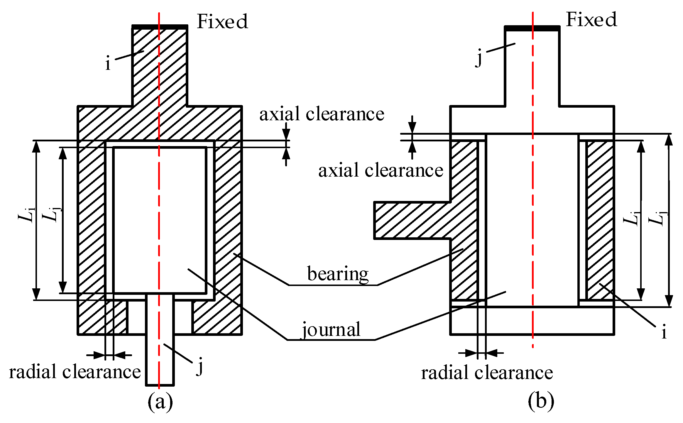
2.1. Combination of Bearing and Journal

According to the practical application of a revolute joint in the production line, Figure 1 shows two combinations of a revolute joint. In Figure 1a, the bearing is fixed and the journal has axial or radial offset with respect to the bearing. In Figure 1b, the journal is fixed and the bearing has axial or radial offset with respect to the journal. The bearing is regarded as a rigid body i and the journal as a rigid body j.

L_i and L_j represent the length of the bearing and journal, respectively. The radial clearance between them is represented by C_r and the axial clearance is represented by C_a. Here, radial and axial clearances are very small, and they are not of the same order of magnitude as bearings and journals.

$$C_r=R_i-R_j$$

(1)

$$C_a=\frac{\left|L_i-L_j\right|}{2}$$

(2)

where the bearing radius is R_i and the journal radius is R_j. In order to facilitate the calculation, Figure 1a is taken as an example. In Figure 1a, the journal length is less than the bearing length, thus Equation (2) can be rewritten as follows:

$$C_a=\frac{L_i-L_j}{2}$$

(3)

According to the three contact modes of point contact, line contact, and surface contact, there are 12 possible contact forms in a revolute joint, as shown in Figure 2.

Any of the above contact forms will cause a certain degree of constraint on the movement of the revolute joint, which will cause a certain error in the movement. The 12 contact forms do not occur simultaneously during the movement. The contact type between the bearing and journal depends on their values and the clearance between them.

2.2. Contact Conditions of Journal and Bearing

As shown in Figure 3, there are three modes of matching between the revolute joint journal and the bearing during rotation. They are free flight mode, continuous contact mode, and pseudo penetration mode. The first mode refers to the mode in which the journal and bearing do not make contact completely during the rotation, as shown in Figure 3a. The continuous contact mode is the mode in which the bearing and journal make contact, but do not deform during the rotation, as shown in Figure 3b. The pseudo penetration mode refers to the mode wherein the bearing and journal deform to a certain extent as a result of the contact force during the rotation, as shown in Figure 3c.

When the revolute joint is in the first mode, the contact force between the two is nonexistent. When the revolute joint is in the other two modes, they will be affected by the contact force. The state of the revolute joint can be resolved by the contact force. It can be seen that the contact force is crucial. Before judging the magnitude of the contact force, the geometric state of their mutual cooperation can be analyzed first.

Figure 4 shows the geometric model of the bearing and journal in the revolute joint. In Figure 4, θ represents the included angle between the axis of bearing and the axis of journal and point M represents the intersection of the two axes. When θ is zero, the fit is divided into two states, namely, axis parallel and coincidence. When θ is not zero, we consider the two axes to intersect at point M. Here, the matching state of the journal and bearing can be divided into two cases: the intersection state of the two axes and the parallel state of the two axes.

In the first case:

A_i and B_i represent the centers of two end-facing circles of the cylinder inside the bearing. A_j and B_j represent the centers of the two end-facing circles of the journal. d₁ is the vector from M to A_j. a is the projection of the mode of vector d₁ on the right end face of the inner cylinder of the bearing. b is the projection of journal radius A_jP_r on the right end face of the inner cylinder of the bearing.

Q and P_r are the lowest point of the right end circle of the cylinder inside the bearing and the lowest end circle of the right end circle of the journal in Figure 4, respectively.

Obviously, point P_r is the closest point of the journal to the bearing in the radial direction. The auxiliary plane τ₂ along point Q is perpendicular to the right end face of the inner cylinder of the bearing. The auxiliary plane τ₁ along point P_r is parallel to plane τ₂, thus the distance from plane τ₁ to plane τ₂ is the distance from point P_r to plane τ₂, which is called the minimum distance between the bearing and the journal in the radial direction, denoted as δ_r, as shown in Equation (4):

$${\delta }_r=R_i-\left|{\mathit{d}}_{\mathit{i}}\right|\sin \theta -R_j\cos \theta$$

(4)

m is the projection of the mode of vector d₁ on the axis A_iB_i. n is the projection of journal radius A_jP_a on the axis A_iB_i of the bearing. P_a is the most right point of the journal and the closest point to the bearing in the axial direction. The distance between P_a and the inner surface of the bearing is expressed by δ_a, which is called the minimum distance between the bearing and the journal in the axial direction. Its expression is shown in Equation (5):

$${\delta }_a=\left|M{A}_i\right|-\left|{\mathit{d}}_{\mathit{i}}\right|\cos \theta -R_j\sin \theta$$

(5)

In the case of the two axes being parallel:

Figure 5 shows the fit condition when the two axes are parallel to each other. The specific values of δ_r and δ_a are easier to analyze than when the two axes intersect. When the two axes are parallel, point N_i and point N_j are the midpoints of the axis of the bearing and the axis of the journal, respectively. The angle of |N_iN_j| in the vertical direction is α. The projection of |N_iN_j| in the radial direction is e₁, then e₁ = cos α. The projection in the axis direction is e₂, thus e₂ = sinα. According to the geometric model, δ_a and δ_r when the two axes are parallel can be calculated as follows:

$${\delta }_a=\frac{L_i}{2}-\frac{L_j}{2}-\left|N_i{N}_j\right|\sin \alpha$$

(6)

$${\delta }_r=R_i-R_j-\left|N_i{N}_j\right|\cos \alpha$$

(7)

After obtaining the equations for δ_a and δ_r, it is easy to distinguish the contact conditions of the bearing and journal. The range of δ_r and δ_a values can describe the contact mode, as shown in Inequalities (8) and (9):

$$\left\{\begin{array}{l}{\delta }_r>0\hspace{1em}\mathrm{free} \mathrm{flight} \mathrm{mode}\\ {\delta }_r=0\hspace{1em}\mathrm{continuous} \mathrm{contact} \mathrm{mode}\\ {\delta }_r<0\hspace{1em}\mathrm{pseudo} \mathrm{penetration} \mathrm{mode}\end{array}\right.$$

(8)

$$\left\{\begin{array}{l}{\delta }_a>0\hspace{1em}\mathrm{free} \mathrm{flight} \mathrm{mode}\\ {\delta }_a=0\hspace{1em}\mathrm{continuous} \mathrm{contact} \mathrm{mode}\\ {\delta }_a<0\hspace{1em}\mathrm{pseudo} \mathrm{penetration} \mathrm{mode}\end{array}\right.$$

(9)

It can be seen from Inequalities (8) and (9) that the values of δ_r and δ_a are very critical when discussing the contact mode. If these two formulas are combined, that is to say, radial minimum distance and axial minimum distance of the bearing and journal are considered at the same time, the result is as shown in

Table 1. Contact mode.

Contact Mode	Radial Minimum Distance	Axial Minimum Distance
free flight mode	${\delta }_r>0$	${\delta }_a>0$
continuous contact mode	${\delta }_r=0$	${\delta }_a>0$
	${\delta }_r=0$	${\delta }_a=0$
	${\delta }_r>0$	${\delta }_a=0$
pseudo penetration mode	${\delta }_r<0$	${\delta }_a>0$
	${\delta }_r<0$	${\delta }_a=0$
	${\delta }_r<0$	${\delta }_a<0$
	${\delta }_r>0$	${\delta }_a<0$
	${\delta }_r=0$	${\delta }_a<0$

.

As can be seen from Table 1, when the joint is in the first mode, both δ_a and δ_r are required to be positive. When the contact mode of the bearing and journal is continuous contact mode, it is necessary to ensure that δ_a and δ_r are not less than zero at the same time. When the contact mode is the pseudo penetration mode, at least one of δ_a and δ_r must be negative. When the bearing and journal are in continuous contact mode or pseudo penetration mode, there will be impact forces between them, which will affect the motion state of the system to varying degrees. Therefore, it is crucial to analyze the impact force for the movement performance of the whole mechanical system.

3. Contact Force Analysis

During the operation of a mechanical system, there will inevitably be different degrees of impact due to the existence of subtle clearances between joints, which will affect the accuracy, efficiency, and service life [24,25,26]. Taking the revolute joint as an example, according to the theory established in Section 2, when the revolute joint is in free flight mode, there is no impact between them [27]. When the bearing and journal are in contact and tend to move with one another, there will be impact force between them [28]. At this point, the impact force could be converted into normal and tangential force according to the geometric state.

3.1. Normal Contact Force Model

A revolute joint with joint clearance can generate heat during its operation. According to the law of conservation of energy, this part of energy generated by heat is lost as heat, and the kinetic energy of the mechanical system containing the revolute joint will be reduced [29]. The famous mechanical model based on elastic theory proposed by Hertz will not be suitable for this kind of motion analysis involving energy dissipation [30]. Based on the mechanical model proposed by Hunt and Crossley [31], the normal contact force model between the bearing and journal can be expressed as follows:

$$F_n=k{\delta }^n+b{\delta }^p\stackrel{•}{{\delta }^{{}_q}}$$

(10)

where δ is the relative deformation and b is the damping coefficient of the mechanical model. The superscript n is the stiffness index, which is resolved by the surface shape and material of the collision object. p and q are the exponents of the damping term. The amount of deformation and impact velocity can affect them. k is the generalized parameter. The parameter is resolved by the geometry dimension and material of revolute joint. It can be acquired by the following equations:

$$k=\frac{4}{3\pi ({\sigma }_i+{\sigma }_j)}{R}^{1/2}$$

(11)

$${\sigma }_l=\frac{1-{\nu }_l^2}{\pi E_l}\hspace{1em}\left(l=i,j\right)$$

(12)

where ν_l and E_l are the Poisson’s ratio and Young’s modulus, respectively. They are determined by the material of the object.

As the center of the cross section of the bearing and the journal is located on the same side of the contact point, the equivalent radius of curvature R of the contact between them can be expressed as follows:

$$R=\frac{R_i{R}_j}{R_i-R_j}$$

(13)

The formula for damping coefficient b is as follows:

$$b=\frac{3k(1-c_e^2){\delta }^n}{4\stackrel{•}{{\delta }^{(-)}}}$$

(14)

where $\stackrel{•}{{\delta }^{(-)}}$ is the initial normal velocity of two objects when they make contact. c_e is the coefficient of restitution. The coefficient is the ratio of their relative velocity after impact to that before in a simple one-dimensional impact when two objects are in pure flat shift.

According to the different values of the parameters k, n, b, p, and q, different mechanical models are established.

When b = 0, Equation (10) becomes the classic Hertz’s model. At this time, the model has two unknown parameters, as shown in Equation (15):

$$F_n=k{\delta }^{{}_n}$$

(15)

When n = 1 and b = 0, Equation (10) becomes the classic spring model. At this time, the model has one parameter, as shown in Equation (16):

$$F_n=k\delta$$

(16)

When n = 1, q = 1, and p = 0, Equation (10) becomes a simple linear spring damping model with two parameters, as shown in Equation (17):

$$F_n=k\delta +b\stackrel{•}{\delta }$$

(17)

When n = 3/2, p = 0, and q = 1, Equation (10) becomes the contact model derived by Lankarani-Nikravesh in 1990 [32]. Then, the model has two parameters, as shown in Equation (18). This equation will be used in this paper.

$$F_n=k{\delta }^{3/2}+b\stackrel{•}{\delta }$$

(18)

By combining Equations (11)–(13) and (18), Equation (19) can be obtained:

$$F_n=k{\delta }^{3/2}\left(1+\frac{3(1-c_e^2)}{4\stackrel{•}{{\delta }^{(-)}}}\right)$$

(19)

3.2. Tangential Contact Force Model

In the joint, when the journal moves in a circular motion inside it, the contact force will be generated between the journal and the bearing as a result of the collision. At this time, a tangential component force will be generated [33]. According to the modified Coulomb friction law [22], the expression of the tangential component is as follows:

$$F_t=-\mu (v_t)F_n\mathrm{sgn}(v_t)$$

(20)

where sgn(v_t) is the symbolic function of the velocity v_t. μ(v_t) is a generalized friction coefficient and a function of v_t, which can be expressed as follows:

$$\mu (v_t)=\left\{\begin{array}{lll}0& \mathrm{for}& \left|v_t\right|\le v_0\\ {\mu }_d\frac{\left|v_t\right|-v_0}{v_1-v_0}& \mathrm{for}& v_0\le \left|v_t\right|\le \\ 1& \mathrm{for}& \left|v_t\right|\ge v_1\end{array}\right.v_1$$

(21)

where v₀ and v₁ are the lower and upper bounds of tangential velocity, respectively, and μ_d is the coefficient of kinetic friction.

4. Dynamic Modeling of Assembly Robot with Joint Clearance

As shown in Figure 6, a SCARA assembly robot with four DOFs is installed in the wine box production line to assemble the base of the wine box. The robot sucks up the bottom sticker of the pedestal through the suction cup at the end and then accurately places the bottom sticker on the base model with glue through a certain trajectory. After the glue solidifies, the assembly of a finished base is complete.

Figure 7a shows that the robot base is bolted to the production line; arm 1 is connected to the base through joint A, arm 2 is connected to arm 1 through joint B, and the end of arm 2 is connected to arm 3 through joint C. Joint A and joint B belong to the revolute pair and joint C belongs to the cylindrical pair. The frame O−XYZ is constructed at joint A on arm 2. O is the center of the upper cylindrical surface where joint A and arm 2 make contact. The Z axis is the rotation axis of joint A; the direction is upward. The X axis coincides with the line of joint A and joint B, and the Y axis is established through the right hand rule. When joint A, joint B, and joint C do not have joint clearance, the multi-body system has only one topology; otherwise, the multi-body system will have a variable topology. As shown in Figure 7b, the SCARA robot grasps the bottom sticker of the wine box through the suction cup on the end effector. Figure 8 shows the specific action process of the SCARA robot.

Assuming that joint A and joint C are both perfect joints and only joint B has joint clearance, the states of joint B during movement can be divided into the three modes mentioned above. When in the first mode, the dynamic equation is as follows:

$$M(q)\stackrel{••}{q}+C(q,\stackrel{•}{q})\stackrel{•}{q}+Q(\stackrel{•}{q})+G(q)=F(t)$$

(22)

where F(t) represents the generalized force matrix; q represents the generalized coordinate vector; M(q) is the mass matrix; C(q,$\stackrel{•}{q}$) is the Coriolis matrix; Q($\stackrel{•}{q}$) is the friction torque; and G(q) is the gravity matrix, namely the gravity factor of each member on the mechanical arm.

When in continuous contact mode and pseudo-penetration mode, the right term of dynamic Equation (22) will change, and the result is shown in Equation (23):

$$M(q)\stackrel{••}{q}+C(q,\stackrel{•}{q})\stackrel{•}{q}+Q(\stackrel{•}{q})+G(q)=F(t)+F_C$$

(23)

where the term F_C added to the right side of the equation contains two parts. F_n is the normal force and F_t is the tangential force.

5. Results and Discussion

The motion state of 3D revolute joint B with different joint clearances of the SCARA robot during the assembly of the wine box base is analyzed in this section. Assuming that all arms of the SCARA robot are rigid, and the rest of the kinematic pairs are perfect,

Table 2. Geometric dimensions and quality attributes of the robot arms.

Arms	Length [mm]	Mass [kg]	Characteristics of Inertia [kg m2]
			Jxx	Jyy	Jzz	Jxy	Jxz	Jyz
Arm 1	329	5.78	2.569	3.080	2.537	2.002 × 10−5	2.384	0.007 × 10−5
Arm 2	275	4.35	1.346	0.981	1.298	4.871 × 10−4	−2.258 × 10−4	−4.22 × 10−4
Arm 3	350	3.03	2.087 × 10−2	2.087 × 10−2	4.726 × 10−5	1.005 × 10−6	3.307 × 10−6	0.489 × 10−6

lists the geometric dimensions and quality attributes of each arm.

Table 3. Dynamic simulation parameters of the assembly robot.

Parameter	Value
Coefficient of friction	0.1
Integration step size	1 × 10−5 s
Young’s modulus	207 GPa
Integration tolerance	1 × 10−7
Coefficient of restitution	0.9
Poisson’s ratio	0.3

lists the simulation parameters of the SCARA robot.

Table 4. Clearance dimension of joint B.

Case	Clearance Dimension (mm)
Case 1	Ca = Cr = 0.2
Case 2	Ca = Cr = 0.5

lists the clearance dimensions of 3D revolute joint B.

When there are clearances of different sizes in joint B, the movement trajectory of the end effector of the SCARA robot will change to different degrees. Figure 9a–c show the displacement change curves of the geometric center of the end effector along the X, Y, and Z axes, respectively, in the O−XYZ coordinate system during the completion of an operation cycle of the robot. In Figure 9, the motion trajectory of joint B with no clearance is shown by the red curve, the motion trajectory of joint B with clearance C_a = C_r = 0.2 mm is shown by the blue curve, and the motion trajectory of joint B with clearance C_a = C_r = 0.5 mm is shown by the magenta curve. As can be seen in Figure 9, when joint clearance is present, the displacement trajectory will fluctuate slightly. The displacement trajectory when joint clearance is 0.2 mm has smaller fluctuation than that when joint clearance is 0.5 mm.

Figure 10a–c show the velocity variation curves of the geometric center of the end effector of the SCARA robot along the X, Y, and Z axes, respectively, in the frame O−XYZ. Through comparison, it can be found that the joint clearance of different sizes has different influences on the velocity, and the joint clearance of 0.5 mm has a greater influence on the velocity.

According to Figure 9 and Figure 10, the size of joint clearance has a decisive influence on the kinematics analysis of the SCARA robot. The displacement and velocity fluctuations of the robot are also different as a result of the different clearances. The smaller the clearance, the smaller the fluctuation of displacement and velocity will be and the better the smoothness of the robot’s movement will be, and the defective rate on the production line will gradually increase.

According to Figure 7, the projection of the sucker in the XOY plane is a square. Figure 11 studies the path of the end effector by studying the path of the geometric center of the square. It can be seen from Figure 11 that, when the clearance of joint B is 0.2 mm, the deviation of the running trajectory is smaller than that when the clearance is 0.5 mm. However, the overall fluctuation at 0.5 mm was slightly better than the fluctuation at 0.2 mm.

Figure 12 shows the path of the journal center running in the bearing under different clearances during the operation of the SCARA robot. In Figure 12, the solid line in red represents the path of the center of the journal in an ideal joint. The blue dotted line inside the circular track composed of red solid lines indicates that the contact mode at this time belongs to the first contact mode, and there is no contact force between them. The part where the blue dotted line coincides with the red solid line represents that the current state is a continuous contact mode, and the blue dotted line belongs to a pseudo penetration mode outside the circular track. These two states can generate different contact forces between them.

Figure 13, Figure 14 and Figure 15 show the variation trend of the bearings and journal of joint B in the X and Y directions, respectively. Figure 13 shows the change in the contact force of joint B in the X direction. By observing the ordinate of Figure 13a,b, it can be found that, when the time t is near 1.6 s and 2.5 s and the clearance is 0.5 mm, the amplitude and fluctuation of the contact force between the bearing and journal are larger. Figure 14 shows the change in the contact force of joint B in the Y direction. By observing the ordinate of Figure 14a,b, it can be found that, when the time t is near 0.2 s and 1.8 s and the clearance is 0.5 mm, the amplitude and fluctuation of the contact force between the bearing and journal are larger. Figure 15 shows the change in the contact force of joint B in the Z direction. By observing the ordinate of Figure 15a,b, it can be found that, when the time t is near 2.1 s and 2.5 s and the clearance is 0.5 mm, the amplitude and fluctuation of the contact force between the bearing and journal are larger.

This characteristic indicates that, the larger the clearance, the greater the influence between the bearing and the journal in the joint, which will directly lead to the reduction in the operating accuracy of the SCARA robot. Then, the constant fluctuation will lead to different degrees of jitter of the end effector of the robot, all of which will decrease the stability, accuracy, and service life of the robot.

6. Conclusions

The kinematic and dynamic characteristics of the assembly robot in the production line of wine box bases are analyzed when one of the joints has joint clearance. The SCARA robot has a total of three joints, among which two joints are revolute joints and one joint is cylindrical. The SCARA robot has four degrees of freedom. In this paper, it is assumed that revolute joint B has radial and axial clearance, so as to study the motion performance of the end effector of the SCARA robot under the influence of relevant joint clearance.

Firstly, 12 possible contact forms are summarized according to the relative positions of the bearings and journal in the revolute joint. Secondly, the contact conditions between the journal and the bearing in the joint with clearance are discussed, and the equation of the minimum distance between their axes is derived under parallel and non-parallel conditions, so as to judge the contact form of the bearing and the journal in both states. Finally, the contact force model is established to simulate the motion state of the end effector of the SCARA robot without joint clearance and with relevant joint clearance. Two types of joint clearances with different sizes are analyzed.

The results show that the smaller joint clearance will increase the motion fluctuation of the end effector of the SCARA robot, and the amplitude is small. The larger joint clearance will increase the motion amplitude of the end effector of the SCARA robot, with less fluctuation. In the actual wine box base production line, the motion fluctuation of the end effector has little influence on the productivity, while the motion amplitude is one of the main factors affecting the productivity. Therefore, the smaller the joint clearance, the smaller the influence on the movement of the robot assembling the wine box base.

References

1. Marques, F.; Isaac, F.; Dourado, N.; Flores, P. 3D formulation for revolute clearance joints. In New Trends in Mechanism and Machine Science; Springer: Cham, Switzerland, 2017; pp. 183–191. [Google Scholar]
2. Vocetka, M.; Bobovský, Z.; Babjak, J.; Suder, J.; Grushko, S.; Mlotek, J.; Krys, V.; Hagara, M. Influence of Drift on Robot Repeatability and Its Compensation. Appl. Sci. 2021, 11, 10813. [Google Scholar] [CrossRef]
3. Pollák, M.; Kočiško, M.; Paulišin, D.; Baron, P. Measurement of unidirectional pose accuracy and repeatability of the collaborative robot UR5. Adv. Mech. 2014, 12, 1687814020972893. [Google Scholar] [CrossRef]
4. Wang, Y.; Pessi, P.; Wu, H.; Handroos, H. Accuracy analysis of hybrid parallel robot for the assembling of ITER. Fus. Eng. Des. 2009, 84, 1964–1968. [Google Scholar] [CrossRef]
5. Qian, W.; Song, S.; Zhao, J.; Hou, J.; Wang, L.; Yin, X. A Study of the Effect of a Kinematic Pair Containing Clearance on the Dynamic Characteristics of a Tool-Changing Robot. Appl. Sci. 2022, 12, 11041. [Google Scholar] [CrossRef]
6. Flores, P.; Ambrósio, J.; Claro, J.C.P.; Lankarani, H.M. Dynamics of Multibody Systems with Spherical Clearance Joints. J. Comput. Nonlinear Dyn. 2006, 1, 240–247. [Google Scholar] [CrossRef]
7. Flores, P.; Ambrósio, J.; Claro, J.C.P.; Lankarani, H.M.; Koshy, C.S. A study on dynamics of mechanical systems including joints with clearance and lubrication. Mech. Mach. Theory 2006, 41, 247–261. [Google Scholar] [CrossRef]
8. Flores, P.; Ambrósio, J.; Claro, J.C.P.; Lankarani, H.M. Translational Joints with Clearance in Rigid Multibody Systems. J. Comput. Nonlinear Dyn. 2008, 3, 011007. [Google Scholar] [CrossRef]
9. Liu, C.-S.; Zhang, K.; Yang, R. The FEM analysis and approximate model for cylindrical joints with clearances. Mech. Mach. Theory 2007, 42, 183–197. [Google Scholar] [CrossRef]
10. Zhang, X.; Zhang, X. Minimizing the influence of revolute joint clearance using the planar redundantly actuated mechanism. Robot. Comput-Int. Manuf. 2017, 46, 104–113. [Google Scholar] [CrossRef]
11. Zhang, X.; Zhang, X.; Chen, Z. Dynamic analysis of a 3-RRR parallel mechanism with multiple clearance joints. Mech. Mach. Theory 2014, 78, 105–115. [Google Scholar] [CrossRef]
12. Erkaya, S. Investigation of joint clearance effects on welding robot manipulators. Robot. Comput.-Int. Manuf. 2012, 28, 449–457. [Google Scholar] [CrossRef]
13. Zhao, B.; Zhou, K.; Xie, Y.-B. A new numerical method for planar multibody system with mixed lubricated revolute joint. Int. J. Mech. Sci. 2016, 113, 105–119. [Google Scholar] [CrossRef]
14. Xiang, W.; Yan, S. Dynamic analysis of space robot manipulator considering clearance joint and parameter uncertainty: Modeling, analysis and quantification. Acta Astronaut. 2020, 169, 158–169. [Google Scholar] [CrossRef]
15. Marques, F.; Isaac, F.; Dourado, N.; Flores, P. An enhanced formulation to model spatial revolute joints with radial and axial clearances. Mech. Mach. Theory 2017, 116, 123–144. [Google Scholar] [CrossRef]
16. Marques, F.; Roupa, I.; Silva, M.T.; Flores, P.; Lankarani, H.M. Examination and comparison of different methods to model closed loop kinematic chains using Lagrangian formulation with cut joint, clearance joint constraint and elastic joint approaches. Mech. Mach. Theory 2021, 160, 104294. [Google Scholar] [CrossRef]
17. Zhao, Y.; Bai, Z.F. Dynamics analysis of space robot manipulator with joint clearance. Acta Astronaut. 2011, 68, 1147–1155. [Google Scholar] [CrossRef]
18. Zhang, H.; Zhang, X.; Zhang, X.; Mo, J. Dynamic analysis of a 3-PRR parallel mechanism by considering joint clearances. Nonlinear Dyn. 2017, 90, 405–423. [Google Scholar] [CrossRef]
19. Askari, E.; Flores, P. Coupling multi-body dynamics and fluid dynamics to model lubricated spherical joints. Arch. Appl. Mech. 2020, 90, 2091–2111. [Google Scholar] [CrossRef]
20. Yan, S.; Xiang, W.; Zhang, L. A comprehensive model for 3D revolute joints with clearances in mechanical systems. Nonlinear Dyn. 2015, 80, 309–328. [Google Scholar] [CrossRef]
21. Akhadkar, N.; Acary, V.; Brogliato, B. 3D revolute joint with clearance in multibody systems. In Computational Kinematics; Springer: Cham, Switzerland, 2018; pp. 11–18. [Google Scholar]
22. Bai, Z.F.; Jiang, X.; Li, J.Y.; Zhao, J.J.; Zhao, Y. Dynamic analysis of mechanical system considering radial and axial clearances in 3D revolute clearance joints. J. Vib. Control 2021, 27, 1893–1909. [Google Scholar] [CrossRef]
23. Bai, Z.F.; Zhao, Y. Dynamic behaviour analysis of planar mechanical systems with clearance in revolute joints using a new hybrid contact force model. Int. J. Mech. Sci. 2012, 54, 190–205. [Google Scholar] [CrossRef]
24. Flores, P. A parametric study on the dynamic response of planar multibody systems with multiple clearance joints. Nonlinear Dyn. 2010, 61, 633–653. [Google Scholar] [CrossRef]
25. Flores, P.; Leine, R.; Glocker, C. Modeling and Analysis of Rigid Multibody Systems with Translational Clearance Joints Based on the Nonsmooth Dynamics Approach. In Multibody Dynamics: Computational Methods and Applications; Arczewski, K., Blajer, W., Fraczek, J., Wojtyra, M., Eds.; Springer: Dordrecht, The Netherlands, 2011; pp. 107–130. [Google Scholar]
26. Ting, K.-L.; Hsu, K.-L.; Wang, J. Clearance-Induced Position Uncertainty of Planar Linkages and Parallel Manipulators. J. Mech. Robot. 2017, 9, 061001. [Google Scholar] [CrossRef]
27. Zhan, Z.; Zhang, X.; Zhang, H.; Chen, G. Unified motion reliability analysis and comparison study of planar parallel manipulators with interval joint clearance variables. Mech. Mach. Theory 2019, 138, 58–75. [Google Scholar] [CrossRef]
28. Qi, Z.; Luo, X.; Huang, Z. Frictional contact analysis of spatial prismatic joints in multibody systems. Multibody Syst. Dyn. 2011, 26, 441–468. [Google Scholar] [CrossRef]
29. Flores, P.; Lankarani, H.M. Dynamic Response of Multibody Systems with Multiple Clearance Joints. J. Comput. Nonlinear Dyn. 2012, 7, 031003. [Google Scholar] [CrossRef]
30. Ravn, P. A Continuous Analysis Method for Planar Multibody Systems with Joint Clearance. Multibody Syst. Dyn. 1998, 2, 1–24. [Google Scholar] [CrossRef]
31. Hunt, K.H.; Crossley, F.R.E. Coefficient of Restitution Interpreted as Damping in Vibroimpact. J. ASME Appl. Mech. 1975, 42, 440–445. [Google Scholar] [CrossRef]
32. Lankarani, H.M.; Nikravesh, P.E. A contact force model with hysteresis damping for impact analysis of multibody systems. J. Mech. Des. 1990, 112, 369–376. [Google Scholar] [CrossRef]
33. Kakizaki, T.; Deck, J.F.; Dubowsky, S. Modeling the Spatial Dynamics of Robotic Manipulators with Flexible Links and Joint Clearances. J. Mech. Des. 1993, 115, 839–847. [Google Scholar] [CrossRef]
Figure 1. Combination forms of a revolute joint. (a) The bearing is fixed and the journal has axial or radial offset with respect to the bearing. (b) The journal is fixed and the bearing has axial or radial offset with respect to the journal.
Applsci 13 02211 g001
Figure 2. Possible contact forms between the bearing and journal. (ad) Two-point contact forms; (e,f) single-point contact forms; (g,h) three-point contact forms; (i) four-point contact form; (j) surface contact form; (k) line contact form; and (l) both surface contact and line contact forms.
Applsci 13 02211 g002
Figure 3. Contact modes.
Applsci 13 02211 g003
Figure 4. The axis of the bearing and journal is not parallel.
Applsci 13 02211 g004
Figure 5. Bearing and journal axes in parallel.
Applsci 13 02211 g005
Figure 6. Assembly diagram of a wine box base.
Applsci 13 02211 g006
Figure 7. Assembly robot and working status. (a) The structure model of the robot; (b) the actual picture of the robot on the production line.
Applsci 13 02211 g007
Figure 8. The specific action process of the SCARA robot.
Applsci 13 02211 g008
Figure 9. Displacement curves of the end effector along the X, Y, and Z axes. (a) The displacement curve along the X−axis direction in the frame OXYZ; (b) the displacement curve along the Y−axis direction in the frame OXYZ; and (c) the displacement curve along the Z−axis direction in the frame OXYZ.
Applsci 13 02211 g009
Figure 10. Velocity curve of the end effector along the X, Y, and Z axes. (a) The velocity curve along the X−axis in the frame OXYZ; (b) the velocity curve along the Y−axis in the frame OXYZ; and (c) the velocity curve along the Z−axis in the frame OXYZ.
Applsci 13 02211 g010
Figure 11. The path of the end effector geometric center in the XOY plane.
Applsci 13 02211 g011
Figure 12. The path track of the journal center inside the bearing: (a) the center trajectory of the journal when both clearances are 0.2 mm and (b) the center trajectory of the journal when both clearances are 0.5 mm.
Applsci 13 02211 g012
Figure 13. Contact force of joint B in the X direction. (a) The contact force in the X direction when both clearances are 0.2 mm and (b) the contact force in the X direction when both clearances are 0.5 mm.
Applsci 13 02211 g013
Figure 14. Contact force of joint B in the Y direction. (a) The contact force in the Y direction when both clearances are 0.2 mm and (b) the contact force in the Y direction when both clearances are 0.5 mm.
Applsci 13 02211 g014
Figure 15. Contact force of joint B in the Z direction. (a) The contact force in the Z direction when both clearances are 0.2 mm and (b) the contact force in the Z direction when both clearances are 0.5 mm.
Applsci 13 02211 g015