Design, Implementation and Validation of a Hardware-in-the-Loop Test Bench for Heating Systems in Conventional Coaches

Abstract

Experimental work with heating systems installed in public transport vehicles, particularly for optimisation and control design, is a challenging task due to cost and space limitations, primarily imposed by the heating hardware and the need to have a real vehicle available. In this work, a hybrid hardware-in-the-loop (HIL) test bench for heating systems in conventional coaches is introduced. This approach consists of a hardware system made up of the main heating components, assembled as a lab experimental plant, along with a simulation component including a cabin thermal model, both exchanging real-time data using a standard communication protocol. This scheme presents great flexibility regarding data logging for further analysis and easily changing the experimental operational conditions and disturbances under different scenarios (i.e., solar irradiance, outside temperature, water temperature from the engine cooling circuit, number of passengers, etc.). Comparisons between the hybrid system’s transient and steady-state responses and those from selected experiments conducted on an actual coach allowed us to conclude that the proposed system is a suitable test bed to aid in optimisation and design tasks. In this context, several closed-loop test experiments using the test bench were additionally carried out to assess the performance of the proposed control system.

1. Introduction

The design, optimisation and control of heating systems installed in conventional public transport vehicles (such as coaches) with internal combustion engines play a key role in maintaining a suitable environment for passenger comfort, considering that these systems must work at different changing operating conditions, e.g., engine speeds that affect the temperature of hot water from the cooling circuit, varying numbers of passengers, solar irradiance, the wide range of outside temperatures (including very low ones), etc. This is of special interest due to the new emission regulations (Euro VI and later), which establish limitations in the availability of hot water until the engine reaches its optimal temperature. Initially, to carry out effective optimisation and control design, it is necessary to obtain dynamic thermal models of both the heating system and the vehicle cabin for offline tuning through simulation and, subsequently, to test their performance experimentally. Hence, prototypes need to be created following the design phase in order to evaluate their performance and determine the feasibility of the system. Once the prototype has been verified, manufacturers can proceed to test the system in real-world conditions [1]. An alternative for the sake of experimentation flexibility and/or when only part of the necessary equipment is available is the use of a hybrid hardware-in-the-loop (HIL) test bench, where some actual elements or components interact with others implemented through modelling and simulation [2].

Modelling of actual HVAC system components (valves, heat exchangers, etc.) is a lengthy and costly task that requires, on the basis of several assumptions, taking into account the physical properties of different fluids (air, water, etc.), the involved energy balance equations, the component geometries and materials or the estimation of thermal parameters from experimental data, among other aspects [3,4]. Different approaches can be found in the literature to obtain the thermal model of a vehicle (car, van or coach) cabin. The most detailed and computationally expensive models are those based on CFD (Computational Fluid Dynamics), which have been used to accurately obtain the evolution of indoor air flows and temperature distribution in order to determine the occupants’ comfort level [5,6,7,8], to analyse the air quality [9,10,11] or to study the influence or effect of certain conditions, such as the thermal insulation properties of the cabin [12] or the opening of doors and windows [13,14]. By contrast, there are lumped models that treat the whole cabin as a single homogeneous zone, primarily intended to assess the impact of the different thermal loads [15] or passenger comfort [16]. Finally, between the two previous types of models, there are those that segment the cabin into several zones, which exchange air volumes, defining lumped models for each one as a simplification of CFD models [17,18,19]; therefore, such exchange mechanisms between adjacent zones must also be mathematically defined. These latter models are a well-suited option for bus or coach cabins, which can be easily partitioned into clearly distinguished air zones, with an optimal balance between accuracy and simplicity with a reasonable computational cost when they are used in the design of control strategies and for real-time simulation.

Therefore, the use of a hybrid HIL test bench made up of the real HVAC system “connected” to a coach cabin thermal model could provide a less costly setup to test control systems and compare different prototypes under the same conditions (number of occupants, solar irradiance, etc.) or the same prototype under different conditions, reducing and improving validation steps. Within the context of HIL test benches for vehicles, several papers can be found in the literature. For example, in [20,21], HIL test benches are employed to validate their proposed electric vehicle battery state-of-charge (SoC) estimation. In [22], the authors developed a HIL setup to validate the effectiveness of a robust fractional-order sliding mode control (RFOSMC) of a hybrid battery/supercapacitor fully active energy storage system (BS-HESS) used in electric vehicles. In [23], an ACC (Adaptive Cruise Control) control strategy is presented and a HIL setup is used, primarily composed of the real braking and driving systems and a dynamic model of an electric bus. However, none of these HIL test benches for vehicles focuses on the HVAC system. On the other hand, several papers can be found describing HIL test benches to evaluate HVAC performance in buildings [1,24,25,26], but not in vehicles. In addition, in [27], the test bench is composed of a real controller and models of the HVAC and the vehicle. In the present work, a virtual controller is used since it provides more flexibility in the evaluation of possible control strategies and structures.

In this research, a highly flexible HIL test bench consisting of the real components of the HVAC system connected to a real-time simulation of a coach cabin thermal model through a standard industrial communication protocol is proposed as the main contribution, making up a hybrid system in which hardware and software components interact with each other through bidirectional real-time data exchange between them. To the authors’ knowledge, a HIL test bench specifically designed and built for public transport coaches that includes actual heating system equipment has not been previously developed. Additionally, the proposed control-oriented cabin thermal model and the validation of the whole system using actual experimental data can be also considered novelties of the work. All this allows for improving the development process of heating systems by reducing and enhancing validation steps, as well as testing the performance of control strategies for these systems at a low cost before their validation on a real coach. Two differentiated air zones (driver and passengers) with bidirectional heat exchange are considered, defining simple lumped models for each one, and OPC UA (Open Platform Communications Unified Architecture) [28] is the industrial protocol used for data communication. The proposed methodology allows for the flexibility of working under different conditions affecting the coach’s thermal model simulation, such as cabin size, number of passengers, solar radiation, etc., so that different scenarios can be considered. The whole system can be used as a test bed to tune and check the performance of any control strategy to be designed, as it is software-implemented, but other potential uses can be also considered, including the assessment of components, optimisation or sensitivity analysis. The authors consider that the proposed methodology is a novelty approach not found in previous state-of-the-art tools for testing the control design of coach heating systems.

The paper is organised as follows. The experimental setup designed for the driver’s zone heating system is detailed in Section 2.1. The proposed model that implements the coach cabin’s thermal behaviour is described in Section 2.2. Selected experiments carried out on a real coach are discussed in Section 2.3, and in Section 3.1, the cabin thermal model is validated. Results of replications of such experiments using the proposed hybrid test bench are detailed and discussed in Section 3.2. The description of results obtained from several illustrative test experiments focused on highlighting the usefulness of the proposed test bench for control system design is presented in Section 3.3. Finally, the conclusions of the work are summarised in Section 4.

2. Materials and Methods

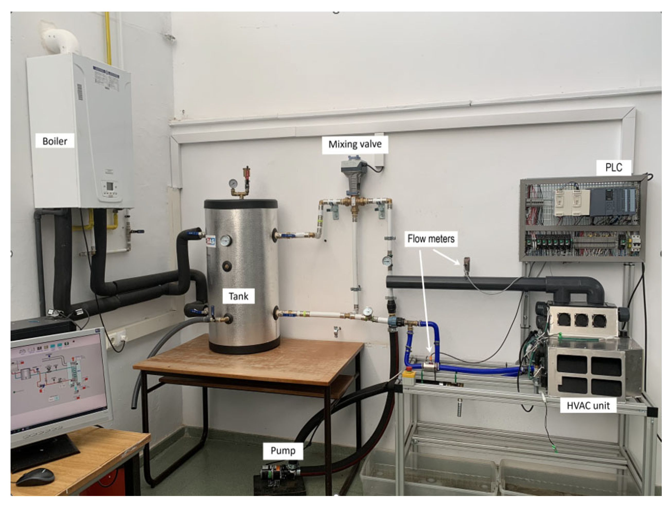
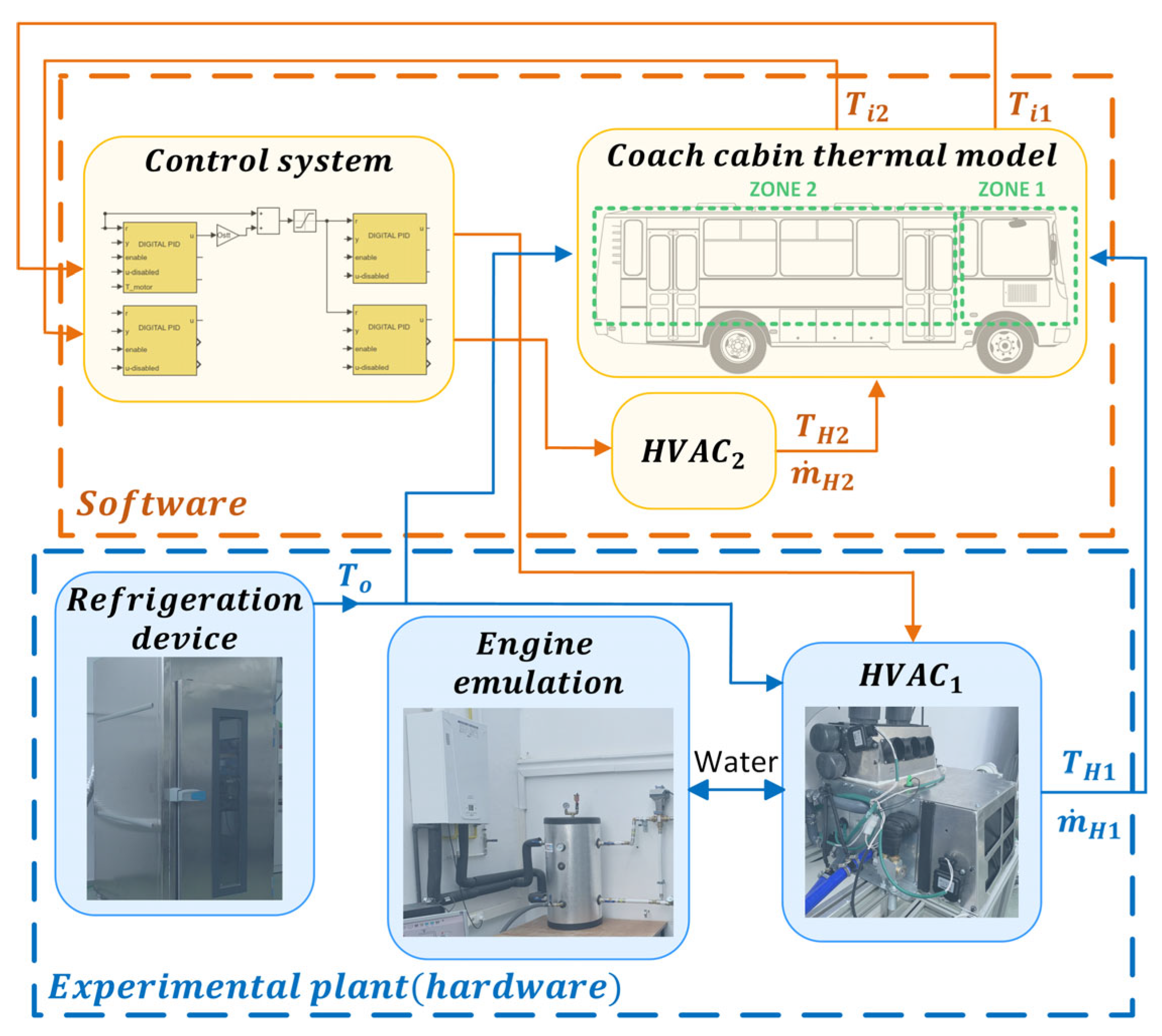
2.1. Experimental Plant

The designed experimental plant, shown in Figure 1 and integrated into the proposed test bench, is located in the Research Laboratory of Automatic Control at the University of Cordoba. The plant primarily consists of an HVAC unit and a water pump, both belonging to a real coach, and a system to emulate the hot water coming from the internal combustion engine cooling circuit, obviously not available in a laboratory. The experimental setup only includes the heating system elements for the driver’s zone because the control of its interior air temperature is more challenging than in the passengers’ zone, for two main reasons: Firstly, the driver discomfort caused by the air and heat exchanges between both zones, with a strong influence of the passengers’ zone on the driver’s one, considering the much smaller air volume in the latter; secondly, the complexity of the control equipment in the driver’s zone is higher (e.g., the valve regulating the hot water flow from the engine cooling circuit is a proportional valve in this zone, while it is an on/off valve in the passengers’ zone). Furthermore, in actual coaches, the HVAC unit installed in the driver’s zone includes security actions involved in glass dehumidification, which is isolated from the passenger system.

A complete set of sensors, more than those that are usually present in actual vehicles, were added to monitor the behaviour of the variables of interest, such as temperatures, flows and pressures. In addition, part of the software needed to run the experimental tests was implemented in a PLC (Programmable Logic Controller). Specifically, the controller was based on a Siemens S7-1512 CPU, which was connected to a PC where the variables of interest were monitored and automatically registered by the SCADA system (created with Siemens SIMATIC WinCC). The low-level operation algorithms of the valve and fans, among other elements, were also implemented in the PLC, and they reproduced exactly what exists in actual vehicles. Furthermore, Matlab/Simulink software (Mathworks, Inc.) was used to implement high-level control strategies and data registering and, of course, the model of the coach thermal dynamics, which will be described in the next section. Finally, the communication between PLC and PC was implemented using the OPC UA protocol.

Figure 2 shows the P&ID (Process & Instrumentation Diagram) of the plant with their main elements and sensor locations. The system incorporated a flowmeter that measured the HVAC unit’s inlet hot water flow rate, and another flowmeter was located at the output hot airflow. The HVAC unit presents a crossflow arrangement, i.e., the ambient air moves perpendicularly to the hot water, which flows through the heat exchanger tubes. Regarding the temperature measurements, four sensors were located at the inlets and outlets of the HVAC unit and a fifth sensor measured the tank temperature, as shown in the diagram.

Table 1. Sensor specifications.

Sensor	Brand/Model	Measured Variable	Measuring Range	Uncertainty
TT-1, TT-2, TT-3, and TT-4	NXP/KTY 81/110	Temperature	−55…+150 °C	±1.27 °C
TI-1	Wika/A43	Temperature	0…120 °C	±2 °C
FT-1	Endress+Hauser/Picomag	Flow rate	0.05…25 L/min	±0.8%
FT-2	IFM/SA5000	Flow rate	0…100 m/s	±7%
PI-1	Mei/CL 1.6	Pressure	0…6 bar	±0.4%

lists the brand, model and other details of the sensors used. In the following section, the main components of the experimental plant are described in detail.

-

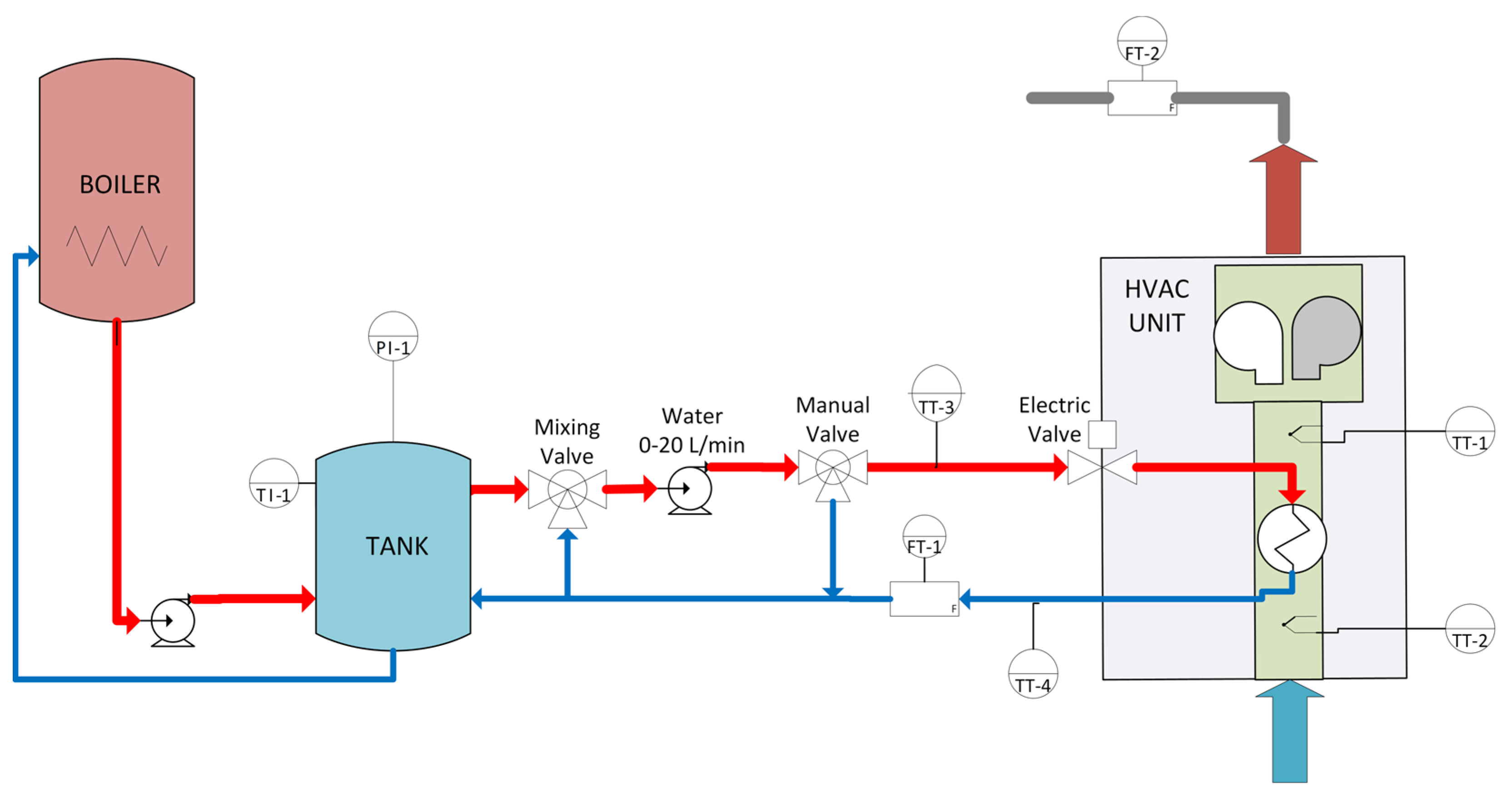
Engine emulation: This subsystem consists of a gas boiler heating unit (24 kW) and a buffer tank (100 L), which allows the emulation of the heat produced by the vehicle’s internal combustion engine through its cooling circuit, being able to produce a constant and continuous hot water flow of 12 L/min at 80 °C. A regulated three-way mixing valve was included at the outlet of the tank to control inlet temperature to the HVAC unit and thus reproduce the behaviour of the engine at start-up, emulating the transitory regime until the steady-state operating temperature is reached. In addition, a water hydraulic pump (the same model of 24 VDC installed in coaches) was used to impulse the hot water to the HVAC unit. Furthermore, a three-way proportional manual valve was included to limit the maximum flow entering the HVAC unit, only added for research purposes (to analyse the effect of changing maximum water flow, reduced in new coaches).

-

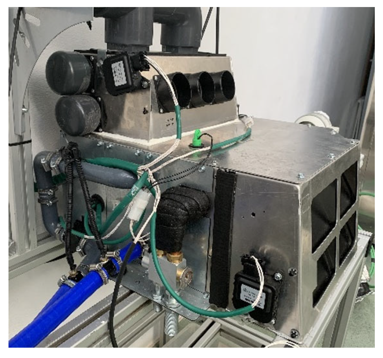
HVAC Unit (Figure 3): This is the main element of the experimental plant. It essentially consists of a water–air heat exchanger, in which heat transfer takes place between the hot water driven by the pump coming from the engine cooling circuit and the outdoor (or recirculated) air. Forced ventilation was carried out by employing two fans, whose speed was varied using Pulse Width Modulation (PWM), to drive the inlet air perpendicularly to the exchanger coil through which the hot water passes. Moreover, this unit had an electric valve to control the inlet hot water flow rate, with this being the main actuator in the temperature or flow (only in the laboratory setting, not in real coaches) control loops. The HVAC unit included two doors whose aperture was controlled by two DC motors; one of these doors was used to control the airflow sent to the vehicle’s front window, intended for dehumidification purposes, for the driver’s feet outputs or a combination of both. The other door was employed to recirculate air from inside the cabin or insert renewal air from outside.

-

Outside temperature emulation: An external refrigeration device was used to impose low-temperature air environmental conditions. This subsystem can keep the inlet constant temperature as low as −10 °C. Forced ventilation was used to direct the cold air from the chamber to the HVAC unit.

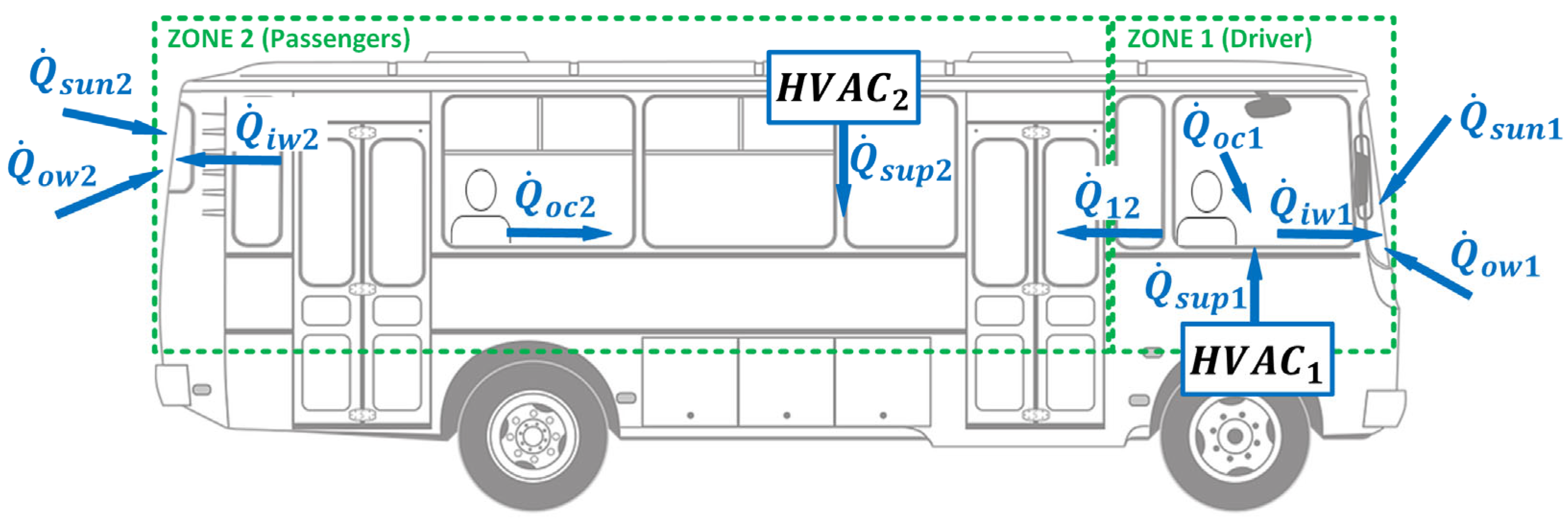
2.2. Proposed Cabin Thermal Model

The thermal model described in this section is based on those introduced in [17] and [19] with several changes and simplifications in order to calculate the mean air temperatures and embed it into the proposed hybrid system for real-time simulation. The coach cabin was divided into two major thermal zones, driver (Zone 1) and passengers (Zone 2), the latter with an air volume much greater than the former. The main novelties of the model introduced in this work are, on the one hand, the existence of inputs (airflow and air temperature) from two different independent heating systems installed on each thermal zone and, on the other hand, the possibility of bidirectional air and heat exchange between such zones. The model is lumped, essentially considering them independent from a thermal point of view and assuming that the different involved temperatures in each zone are uniform, though with mass and energy exchange between them. It is based on energy balance equations primarily considering, in a simplified manner, the interior air volume in each zone, the characteristics of the surrounding window panes embedded into the vehicle body, the number of occupants, the outside temperature, the incident solar radiation and the dimensions of the vehicle, some of which are parameters or disturbances that can be modified for the thermal simulation of the cabin. The outputs of the model are the mean air temperatures of both zones. Figure 4 presents a diagram of the cabin’s thermal model. It shows the two zones and the associated heat loads.

Equations (1) and (2) describe the energy balance for Zone 1. $T_{i1}$, $T_{i2}$ and $T_{w1}$ are the mean interior temperatures of both zones and the temperature of the windows in the driver’s zone, respectively. $C_{i1}$ and $C_{w1}$ are the heat capacities of the air in Zone 1 and of the windowpanes of that zone, respectively, and are calculated using Equations (3) and (4). $V_{i1}$ is the interior air volume in Zone 1, ${\rho }_i$ is the air density, $c_{pi}$ is the specific heat capacity of air, $V_{w1}$ is the window pane volume surrounding the driver’s zone, ${\rho }_{glass}$ is the density of the glass and $c_{pglass}$ is the specific heat capacity of the glass. The terms on the right-hand side of Equations (1) and (2) are the heat transfers and heat loads, which affect the temperature of the air in Zone 1. Constant parameter values from equations regarding the driver’s zone are shown in

Table 2. Values of model parameters from equations regarding Zone 1.

Parameter	Value
$V_{i1}$	12 m3
$V_{w1}$	0.0425 m3
${\rho }_i$	1.225 Kg·m−3
${\rho }_{glass}$	2.5·103 Kg·m−3
$c_{pi}$	1005 J·Kg−1·K−1
$c_{pglass}$	850 J·Kg−1·K−1
$\beta$	1
$A_{12}$	6.25 m2
$H$	2.5 m2
$A_{front1}$	7 m2
$A_{left1}$	2 m2
$A_{right1}$	2 m2

.

$$C_{i1}\frac{d{T}_{i1}}{dt}={\dot{Q}}_{sup1}+{\dot{Q}}_{oc1}-{\dot{Q}}_{iw1}-{\dot{Q}}_{12}$$

(1)

$$C_{w1}\frac{d{T}_{w1}}{dt}={\dot{Q}}_{iw1}+{\dot{Q}}_{ow1}+{\dot{Q}}_{sun1}$$

(2)

$$C_{i1}=V_{i1}·{\rho }_i·c_{pi}$$

(3)

$$C_{w1}=V_{w1}·{\rho }_{glass}·c_{pglass}$$

(4)

${\dot{Q}}_{sup1}$ is the heat load from the air supplied by the heating system in Zone 1 and is calculated using Equation (5).

$${\dot{Q}}_{sup1}={\dot{V}}_{H1}·{\rho }_i·c_{pi}·\left(T_{H1}-\beta ·T_{i1}\right)$$

(5)

where ${\dot{V}}_{H1}$ is the supply volumetric airflow rate, $T_{H1}$ is the temperature of the supplied air and $\beta$ is the ratio of flow rate from recirculation air in Zone 1; both ${\dot{V}}_{H1}$ and $T_{H1}$ are two of the model inputs.

${\dot{Q}}_{oc1}$ is the sensible heat load from the driver (the only occupant in Zone 1); its value is approximately 70 W per person [29]. ${\dot{Q}}_{iw1}$ is the convective heat transfer between the interior air in Zone 1 and the windows embedded in the coach body in that zone. It is calculated using Equation (6),

$${\dot{Q}}_{iw1}=sign\left(T_{i1}-T_{w1}\right)·U_{iw}·A_{w1}·\left|T_{i1}-T_{w1}\right|$$

(6)

where $U_{iw}$ is the overall heat transfer coefficient between the air and the vehicle windows in Zone 1 and is usually empirically obtained [30], $A_{w1}$ is the contact surface area and $T_{w1}$ is the mean temperature of the windows in the driver’s zone. Equation (6) considers the heat transfer direction depending on the difference between the interior air temperature and one of the windows; if such a difference is positive ($sign\left(T_{i1}-T_{w1}\right)=+1$, i.e., $T_{i1}-T_{w1}>0$), the heat transfer occurs from the interior air to the windows and in the opposite direction if it is negative.

${\dot{Q}}_{12}$ is the heat load due to the air temperature difference between Zones 1 and 2, which causes air circulation from one zone to the other due to the stack effect [31], and it is calculated from Equation (7).

$${\dot{Q}}_{12}={\dot{V}}_{12}·{\rho }_i·c_{pi}·\left(T_{i1}-T_{i2}\right)$$

(7)

Volumetric air flow ${\dot{V}}_{12}$ can be calculated from Equation (8) [31], which takes into account the air transfer from the warmer zone to the colder one,

$${\dot{V}}_{12}=sign\left(T_{i1}-T_{i2}\right)·0.03·A_{12}·\sqrt{g·H·\left|T_{i1}-T_{i2}\right|/T_{ref}}$$

(8)

where $A_{12}$ is the contact area between the two zones, $H$ is the height of that area, $g$ is the acceleration of gravity and $T_{ref}=T_{i1}$ if $T_{i1}-T_{i2}>0$ or $T_{ref}=T_{i2}$otherwise; the factor 0.03 has been determined using least-squares estimation from an actual coach’s experimental data. Airflow direction is also considered the same way as in Equation (6), but in this case from the difference $T_{i1}-T_{i2}$ between interior air temperatures of both zones.

${\dot{Q}}_{ow1}$ is the convective heat transfer between the outside air and the windows embedded in the coach body in Zone 1; it can be calculated from Equation (9),

$${\dot{Q}}_{ow1}=sign\left(T_o-T_{w1}\right)·U_{ow}·A_{w1}·\left|T_o-T_{w1}\right|$$

(9)

where $T_o$ is the outside air temperature, which is another model input, $U_{ow}$ is the overall heat transfer coefficient between the outside air and the vehicle windows in Zone 1 and $A_{w1}$ is the surface of those windows. As in previous cases, Equation (9) also considers that heat transfer may occur from any side to the other.

Finally, ${\dot{Q}}_{sun1}$ is the heat transfer due to incident solar radiation over the windows in Zone 1 and is calculated using Equation (10),

$${\dot{Q}}_{sun1}={\alpha }_w·\sum I_{side}·A_{side1} , side=\left(front,right,left\right)$$

(10)

where ${\alpha }_w$ is the absorptivity of the windows, $I_{side}$ is the incident solar irradiance on each side of Zone 1 (front, left and right) dependent on the environmental conditions and $A_{side1}$ is the surface of the corresponding window section. Obviously, $A_{w1}=A_{front1}+A_{left1}+A_{right1}.$

Energy balance equations for Zone 2 (passengers) can be similarly stated as Equations (1) and (2). Specifically, Equations (11) and (12) describe the effect of heat loads and heat transfers on the interior air temperature of Zone 2 ($T_{i2}$) and the temperature of vehicle windows in that zone ($T_{w2}$). $C_{i2}$ and $C_{w2}$ are the heat capacities of the air in Zone 2 and of the windowpanes of that zone and are calculated using Equations such as (3) and (4). Values of additional model parameters from equations regarding Zone 2 are shown in

Table 3. Values of model parameters from equations regarding Zone 2.

Parameter	Value
$V_{i2}$	100 m3
$V_{w2}$	0.325 m3
$A_{back2}$	5 m2
$A_{left2}$	30 m2
$A_{right2}$	30 m2

.

$$C_{i2}\frac{d{T}_{i2}}{dt}={\dot{Q}}_{sup2}+{\dot{Q}}_{oc2}-{\dot{Q}}_{iw2}+{\dot{Q}}_{12}$$

(11)

$$C_{w2}\frac{d{T}_{w2}}{dt}={\dot{Q}}_{iw2}+{\dot{Q}}_{ow2}+{\dot{Q}}_{sun2}$$

(12)

Equation (13) calculates the heat load from the air supply by the heating system in Zone 2. Both ${\dot{V}}_{H2}$ and $T_{H2}$ are considered additional model inputs, and the recirculation ratio $\beta$ is assumed to be the same as in Zone 1.

$${\dot{Q}}_{sup2}={\dot{V}}_{H2}·{\rho }_i·c_{pi}·\left(T_{H2}-\beta ·T_{i2}\right)$$

(13)

The value of sensible heat load from the passengers (${\dot{Q}}_{oc2}$) is estimated as $n·70$ W, where $n$ is the number of occupants in Zone 2. Equation (14) calculates the convective heat transfer between the air in Zone 2 and the windows surrounding that zone; its structure and the meaning of its terms are the same as in Equation (4), but with parameters and variables corresponding to the passengers’ zone. Similarly, Equation (15) allows us to calculate the convective heat transfer between the outside air and the vehicle windows in Zone 2.

$${\dot{Q}}_{iw2}=sign\left(T_{i2}-T_{w2}\right)·U_{iw}·A_{w2}·\left|T_{i2}-T_{w2}\right|$$

(14)

$${\dot{Q}}_{ow2}=sign\left(T_o-T_{w2}\right)·U_{ow}·A_{w2}·\left|T_o-T_{w2}\right|$$

(15)

The heat transfer provided by solar radiation is obtained from Equation (16). Compared with Zone 1, the back side has been added and the front side has been removed.

$${\dot{Q}}_{sun2}={\alpha }_w·\sum I_{side}·A_{side2} , side=\left(right,left,back\right)$$

(16)

2.3. Experimental Data

Validation of the proposed model was carried out using data provided by a European leader of transport vehicles, specifically by its department of HVAC systems. Most of these data have been obtained from approximately 50 open and closed-loop tests conducted on an actual coach fully equipped with sensors (flowmeters, thermometers, etc.), making trips in cold regions of Europe (Sweden, Poland, etc.) at nearly constant speeds (trying to keep the engine at almost the same regime), as well as static tests inside climate chambers in Germany, covering a suitable range of typical working operating conditions and under different outside temperatures; the experiments were started with a completely stopped and cold engine to deal with the slow reaction capacity of the heating system during the start-up due to the initially low temperature of the water from the cooling circuit (the most sensitive phase of the tests). The model was fed with the actual time profiles for ${\dot{V}}_{H1}$, $T_{H1}$, ${\dot{V}}_{H2}$, $T_{H2}$ and $T_o$ registered from the sensors. The conditions of three selected experiments that are a representative sample of the above-mentioned tests considering low, medium, and high outside temperatures are summarised in

Table 4. Operating conditions of selected validation tests.

Experiment Number	Initial Cabin Temperatures $({\mathit{T}}_{\mathit{i}1\_0}$$/{\mathit{T}}_{\mathit{i}2\_0})$ (°C)	Outside Temperature Range (°C)	Solar Irradiance (W/m2)	Experiment Time of Day	Weather Conditions	Number of Passengers
1	5.2 / 5.7	0–10	0	Night	Foggy	5
2	13.8 / 17.1	7–16	≈200	Noon	Sunny	4
3	18.2 / 19.4	16.5–19	≈200	Afternoon	Sunny	4

, where irradiance values were estimated from databases, taking into account the day and time at which each experiment was performed. A medium-sized coach was considered, and the number of passengers was limited to the research team.

Experiments 2 and 3 were carried out with similar weather conditions and solar irradiance, though the mean outside temperature was higher in the latter, the position of the window/feet door was different (set to 70% in the former and to 2% in the latter) and fan speeds were also varied at certain times during Experiment 3 (they were constant in Experiment 2).

3. Results and Discussion

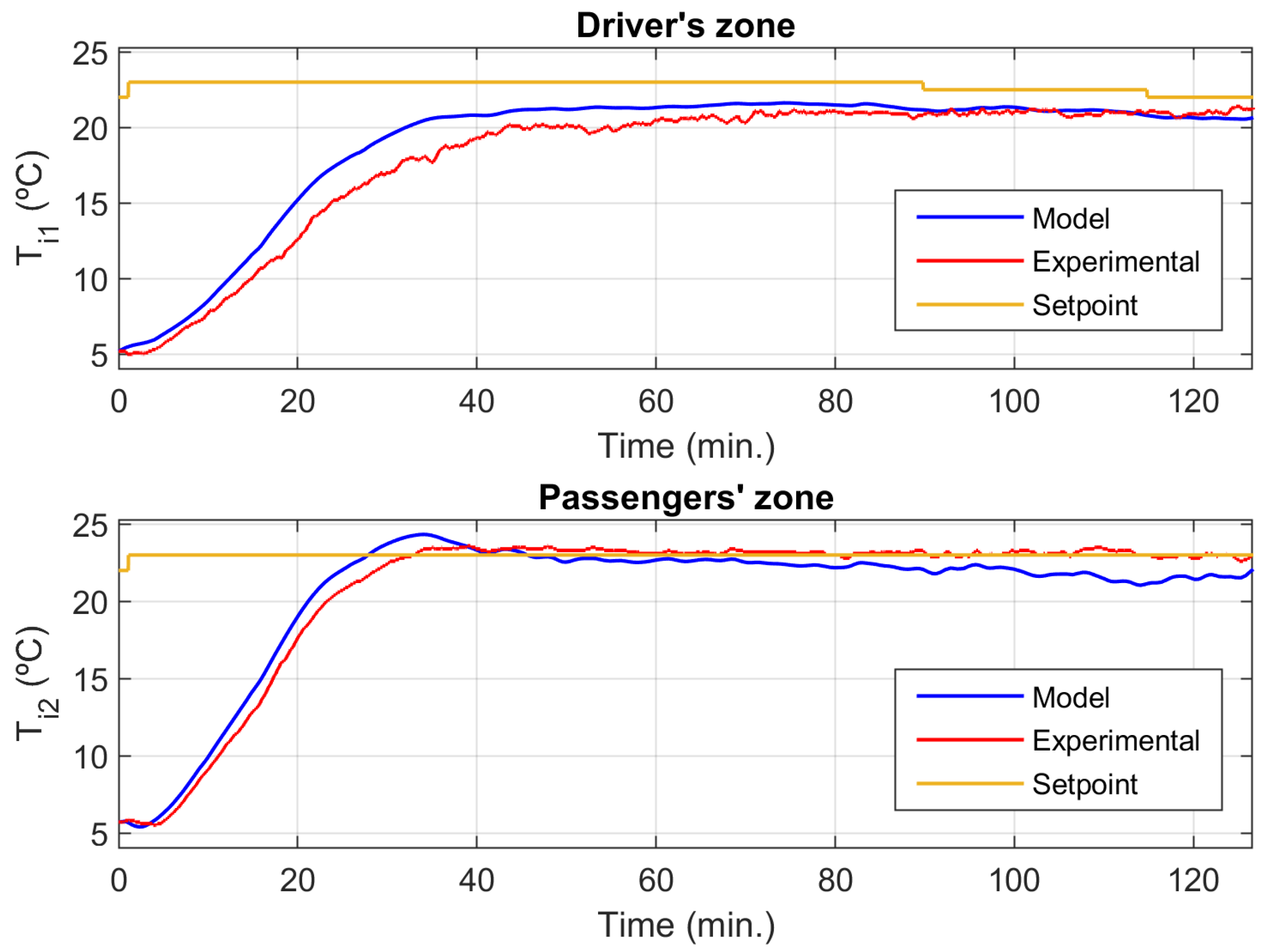
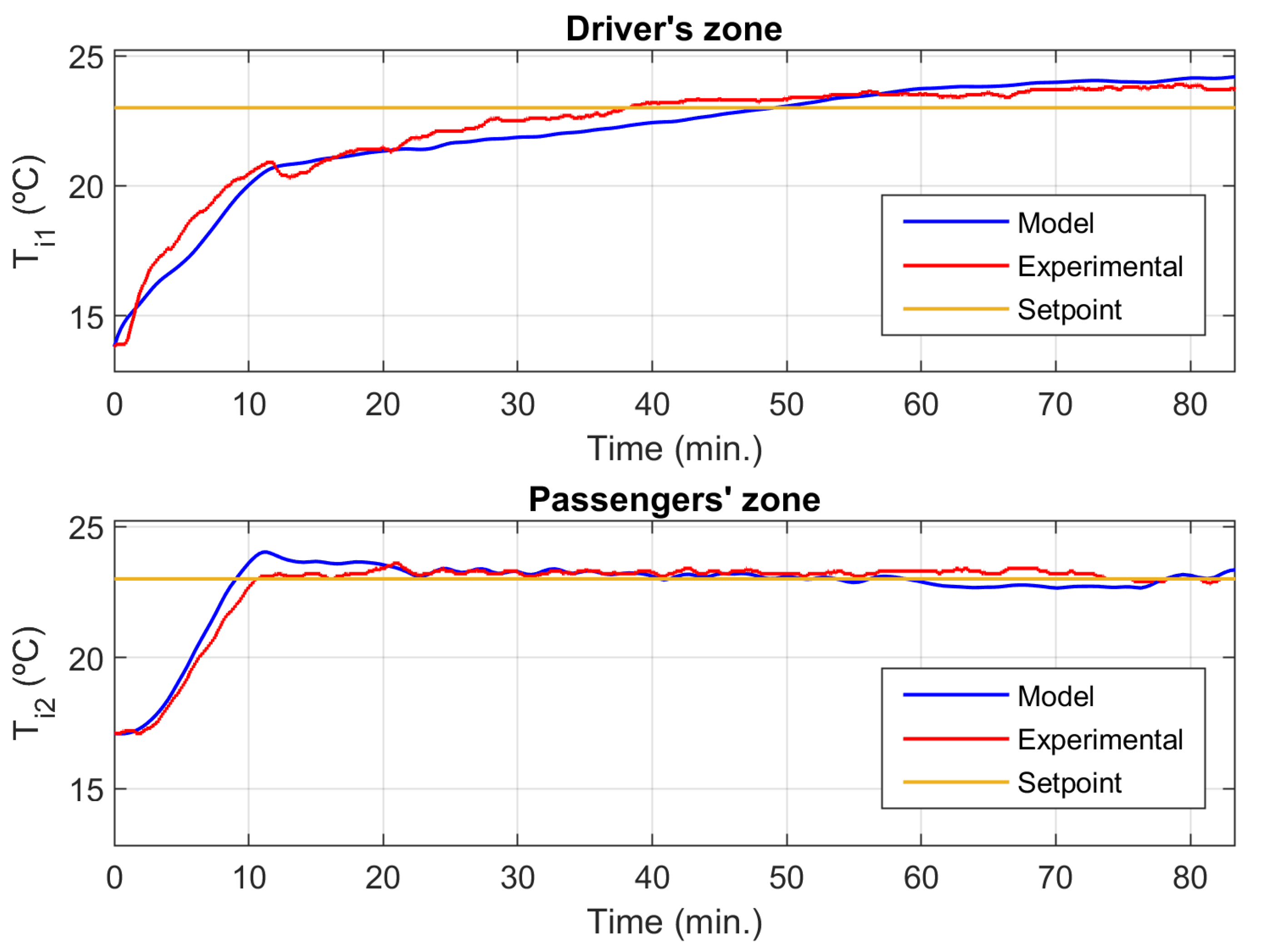
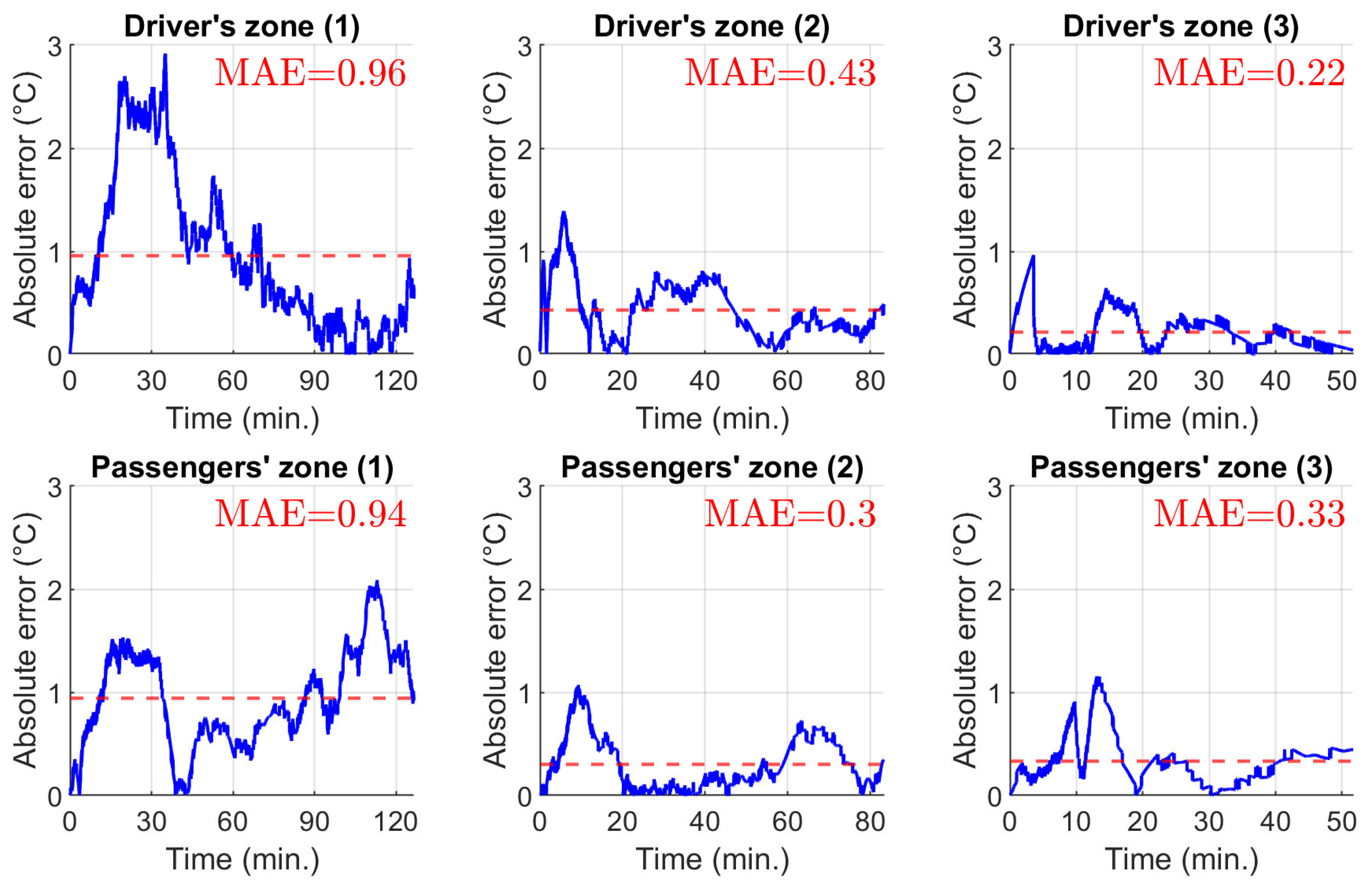
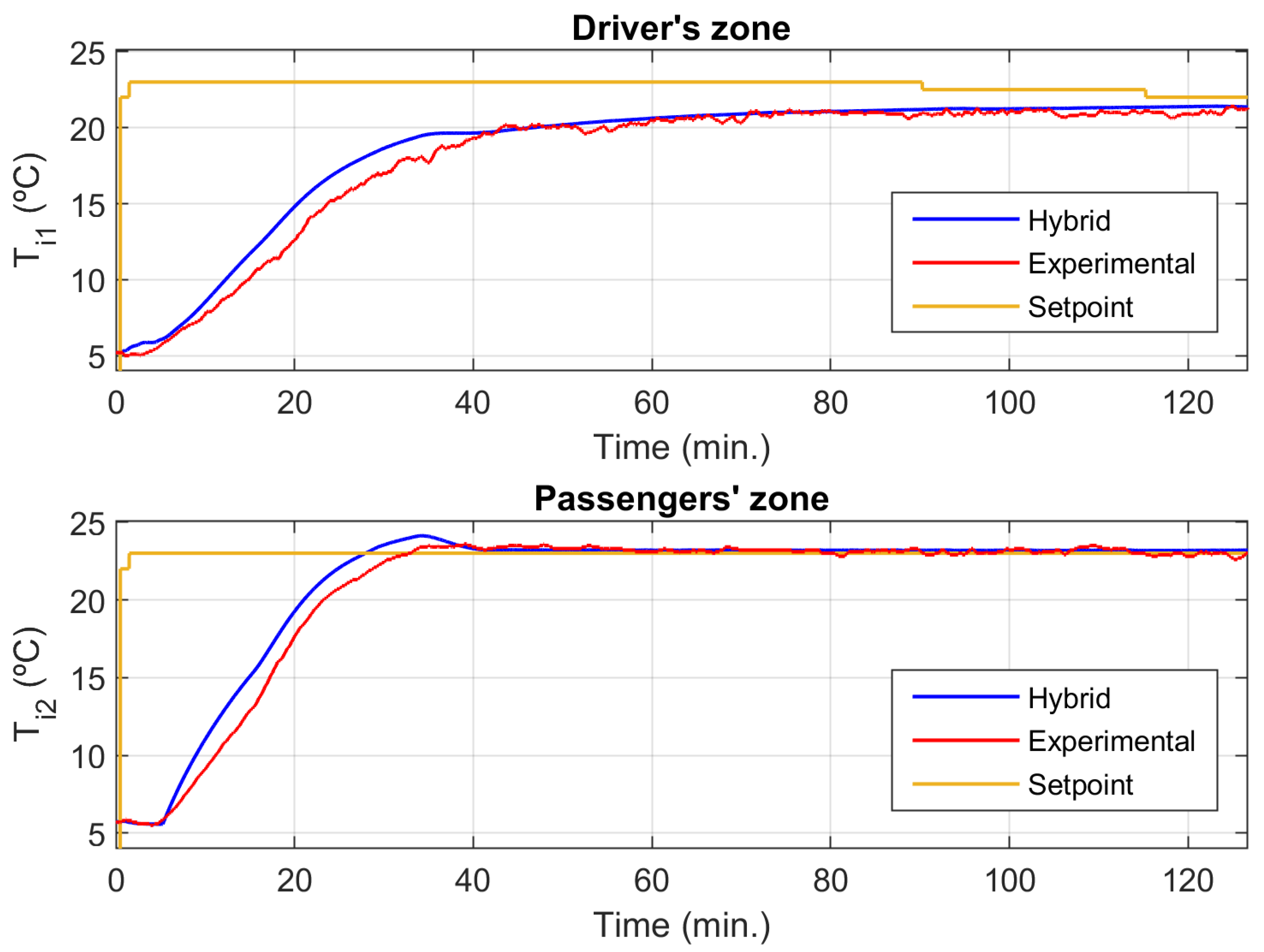
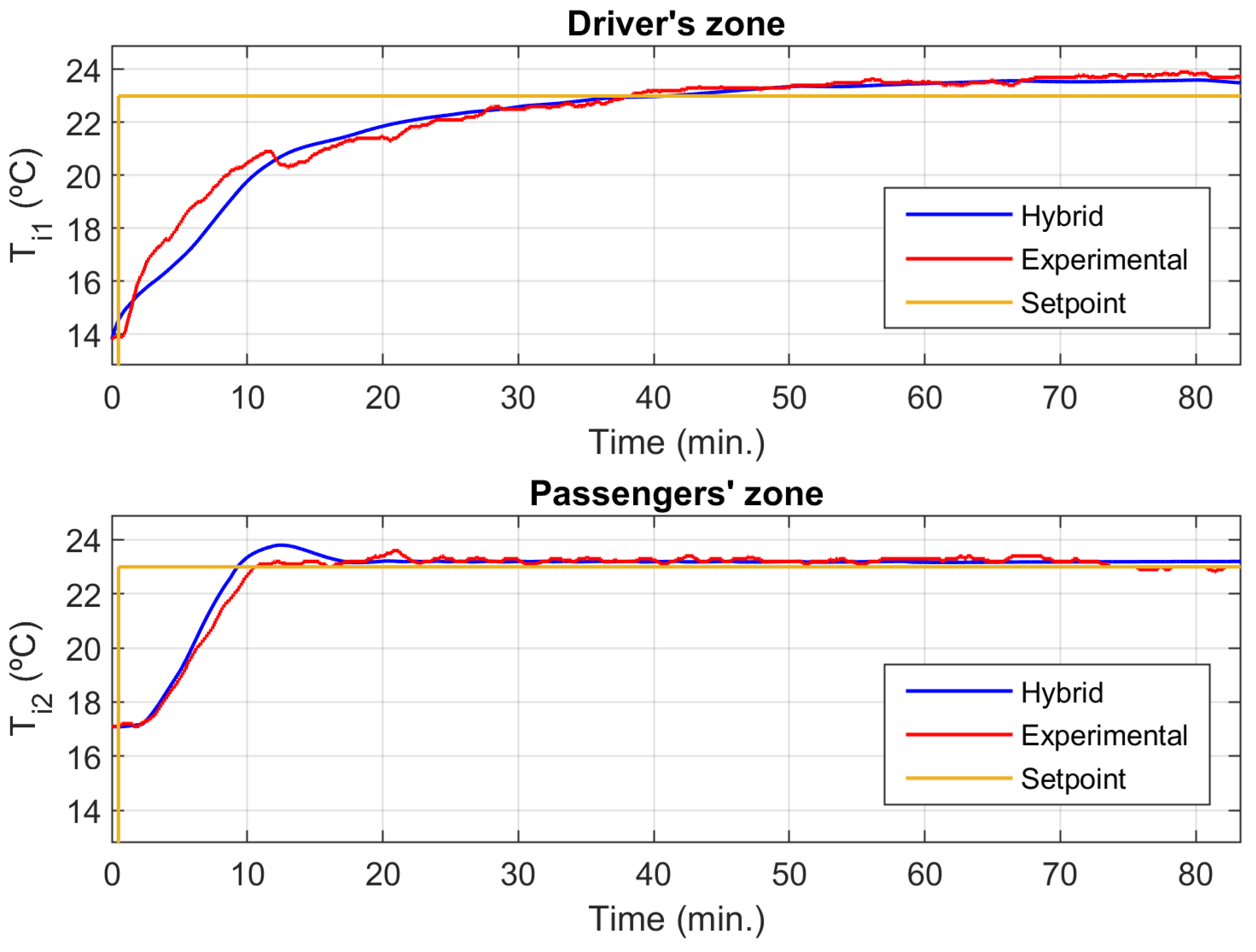
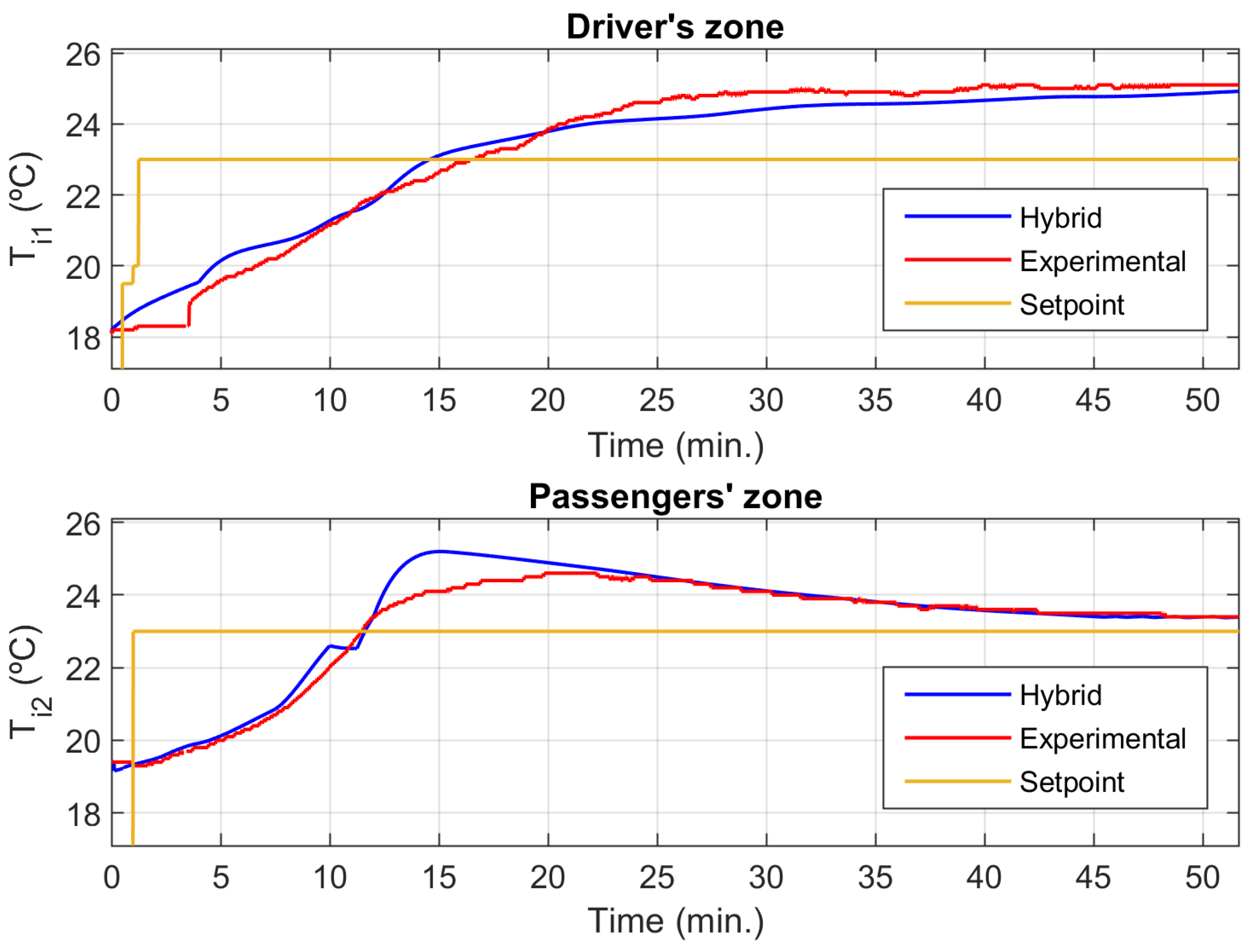
3.1. Model Validation

Comparisons between $T_{i1}$ (temperature of the driver’s zone) and $T_{i2}$ (temperature of passengers’ zone) from the model simulation and from the actual coach cabin for the experiments in Table 4 are shown in Figure 5, Figure 6 and Figure 7, respectively, where the setpoints are also shown. Such simulations were performed using the Simulink environment from MATLAB version R2022a (Mathworks, Natick, MA, USA), where the model was implemented with a masked subsystem shown in Figure 8a and the solver used was an explicit fixed-step fourth-order Runge–Kutta. The unmasked model is also shown in Figure 8b for a better description of its implementation.

Inputs $T\_H1$ and $V\_H1$ in Figure 8a are the temperature of the air and the supplied air flow rate from the heating system of the driver’s zone, respectively. Likewise, inputs $T\_H2$ and $V\_H2$ are associated with the heating system of the passengers’ zone. Lastly, input $T\_o$ is the outside temperature and input $I$ is the irradiance data. On the other hand, outputs $T\_i1$ and $T\_i2$ are the simulated indoor mean temperatures of both thermal zones, respectively.

Heat transfer coefficients and absorptivity were tuned using least-squares estimation from the experimental data, obtaining $U_{iw}$ ≈ 8 W·m⁻²·K⁻¹, $U_{ow}$ ≈ 3 W·m⁻²·K⁻¹ and ${\alpha }_w=$ 0.19.

As can be seen from Figure 5, Figure 6 and Figure 7, there is a close similarity between the model simulation and the experimental data for both transient behaviour and the steady state in the driver and passenger zones; minimal differences can be observed only at certain time intervals or instants for all experiments, often due to certain operational changes that cannot be accounted for in the model simulation; for example, variations in the engine temperature due to changes in vehicle speed. The maximum errors and the mean absolute errors (MAEs) between the experimental and simulated temperatures for each experiment are shown in

Table 5. Performance indices of selected validation tests from model simulation and actual experimental coach data.

Experiment Number	Driver’s Zone		Passengers’ Zone
	Max. Error (°C)	MAE (°C)	Max. Error (°C)	MAE (°C)
1	2.92	0.96	2.09	0.94
2	1.39	0.43	1.07	0.30
3	0.97	0.22	1.16	0.33

to quantify their similarity, which is also graphically shown in Figure 9. In experiments 2 and 3, the MAEs are close to zero and the maximum errors are approximately 1 °C, so they are not very significant. In experiment 1, however, the discrepancies are greater, but the MAEs still remain below 1 °C. This might be due to the irradiance parameter, which was not considered a tuning parameter in this experiment. The same results were reached with other tests, so the proposed model can be considered validated within the range of analysed working operating conditions.

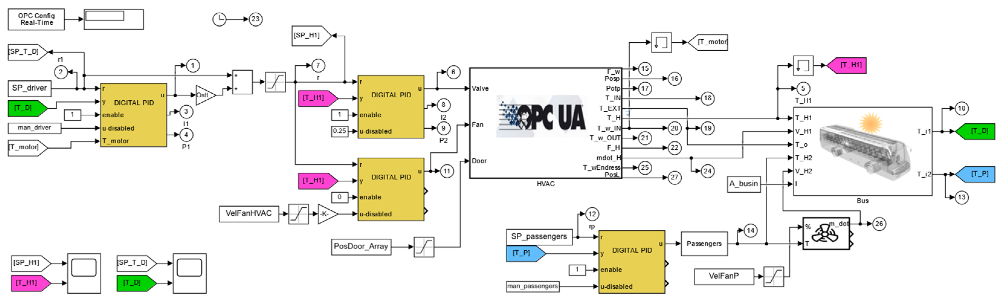
3.2. Hybrid Hardware-in-the-Loop Test-Bench

Once the model introduced in Section 2.2 was validated under different conditions, the experimental setup described in Section 2.1 was “connected” with its real-time simulation to conform the whole proposed hybrid hardware-in-the-loop test bench. Figure 10 illustrates the main elements used in the HIL test bench, with a clear distinction between the hardware and software components. It also displays the data exchanged between the coach cabin model, the heating systems and the control system.

A Simulink model was created (see Figure 11), including the coach cabin’s thermal model, an OPC UA block to connect with the heating system hardware of the driver’s zone (i.e., it represents the built experimental plant within the Simulink block diagram) and the PID controllers required to implement the same control system found in a real coach; “Simulink Desktop Real-Time”, “Industrial Communication” and “Control System” toolboxes were used for real-time simulation and OPC communications, respectively. Such a Simulink model only implements the cascaded control structure for the driver’s zone in detail, while that of the passengers’ zone is represented with a single PID because only the HVAC unit of the driver’s zone was available in the laboratory, as described in Section 2.1. The digital PID controller blocks were designed by the authors and their typical capabilities were implemented, including an anti-windup mechanism and a derivative filter, among others. Such blocks are implemented using code embedded in MATLAB functions for two reasons: Code is easier to translate to C++, the language in which the controllers are programmed in onboard systems, and the possibility to implement more complex algorithms in that way, such as gain scheduling integral action during the start-up sequence or in the dehumidification procedure, to cite two examples.

The OPC UA block is configured as a client connected to the PLC, which is the OPC UA server, which interacts with the plant. This block has two main inputs: The valve opening to vary the hot water flow from the engine cooling circuit and the supply air fan speed. It has several outputs, the most important being the supply airflow rate and the supply air temperature, which are provided to the corresponding inputs of the cabin thermal model block (driver’s zone). Other outputs not fed to the coach cabin model are configured in the OPC UA block for logging and analysis purposes. Under this consideration, the cooling valve position, flow rate and input/output temperatures of the water through the heat exchanger, etc., are included.

Replications of actual tests from Table 4 were carried out to validate the proposed hybrid system and verify its usefulness as a test bench. In this context, the mean of experimental outside temperatures was considered and the temperature of the water coming from the engine cooling circuit was replicated, including the start-up time span, setting suitable setpoints on the boiler and mixing with cold water at predefined time instants. Initial conditions (such as initial temperatures of both coach cabin model zones) were also taken from experimental data, as well as fan speeds and temperature setpoints for driver and passenger zones.

Figure 12, Figure 13 and Figure 14 show the results obtained comparing the actual experimental coach cabin temperatures with those from the test bench.

As can be seen from the above figures, there is a close similarity between the temperature transient time responses and steady states in both zones from the hybrid test bench and the actual experimental coach data.

Table 6. Performance indices of selected validation tests from hybrid test bench and actual experimental coach data.

Experiment Number	Driver’s Zone		Passengers’ Zone
	Max. Error (°C)	MAE (°C)	Max. Error (°C)	MAE (°C)
1	2.35	0.57	2.39	0.46
2	1.58	0.28	0.91	0.17
3	1.13	0.35	1.13	0.21

shows the MAEs and maximum errors. Small variations can be observed with respect to the simulation results introduced in Figure 5, Figure 6 and Figure 7, justified by the simplification of the outside temperature profiles and slight differences in the tuning of the PID controllers, with a better performance in general in the test bench. Table 6 and Figure 15 show that the MAE are close to zero in all the experiments. Similar results were obtained when comparing them with other experiments under different operating conditions; thus, the proposed hardware-in-the-loop system can be considered a valid and efficient test bed to check the performance of any control and optimisation strategy to be designed in the future.

3.3. Test Experiments

Additional experiments were carried out using the proposed test bench to assess, by way of example, the performance of the cascaded closed-loop control scheme for the driver’s zone shown in Figure 11, tuned by the authors under different conditions; specifically, temperature transient and steady-state responses in the presence of setpoint changes both in driver and passenger zones, outside temperature and solar irradiance were analysed.

Time responses of the interior air temperature of driver and passenger zones ($T_{i1}$ and $T_{i2}$, respectively) are shown in Figure 16 for the first proposed experiment, where the driver’s zone setpoint was initialised at 21 °C and, subsequently, was changed to 23 °C around time = 166 min. The temperature setpoint for the passengers’ zone was kept constant at 22 °C, the outside temperature was between 6.5 °C and 11.5 °C and a low, uniformly distributed (the same for all sides) solar irradiance was set to 50 W.

Suitable setpoint tracking for $T_{i1}$ and $T_{i2}$ can be observed in Figure 16, where temperature changes in the driver’s zone barely have an impact on the passengers’ zone; additionally, the time response is slower in the former, primarily due to the strong influence from the latter, with a larger air volume, which is a well-known fact from previous experience.

Complementarily, the passengers’ zone setpoint changed from 21 °C to 23 °C around time = 166 min in the second proposed test experiment, keeping the setpoint constant for the driver’s zone to 22 °C (Figure 17); all other conditions were almost the same as in the first experiment, with minimal variation regarding the outside temperatures. It can be observed from Figure 17 that there are significant impacts of the passengers’ zone temperature changes on the driver’s zone and how the control system is able to bring its interior air temperature back to its setpoint. This effect completely reproduces the real coach dynamics, showing this unidirectional strong interaction.

For the third proposed test experiment, the temperature setpoint was set to 21 °C both in the driver and passenger zones and the outside temperature was gradually reduced from 10.5 °C to 2.8 °C beginning at time = 170 min and ending at time ≈200 min, while maintaining a uniform solar irradiance of 50 W. The results obtained are shown in Figure 18.

As can be seen, the applied disturbance was effectively rejected in both zones, but with a much slower response for $T_{i1}$, even more than in other experiments. In addition to the lower volume present in the driver’s zone, in this case, the outside air also cools down the water coming from the engine, which is the heat source of the heating system, slowing down its reaction.

Solar irradiance was varied in the fourth test experiment, where a setpoint of 23 °C was used for both zones and the outside temperature ranged between 8.1 °C and 17.9 °C. Null irradiance was initially imposed, and then it was linearly changed beginning at time = 166 min and ending around time = 171 min, achieving 50 W (front) and 500 W (remaining sides). The obtained interior air temperatures of the driver and passenger zones along with their setpoints are shown in Figure 19.

It can be observed from the previous figure that the disturbance was effectively rejected in both zones using the control loop scheme shown in Figure 11, with a slower response for $T_{i1}$ due to the lower air volume in the driver’s zone. Therefore, it can also be seen that, despite its much higher value for the passengers’ zone, solar irradiance has a much smaller influence in comparison with the driver’s zone, where a similar impact is observed but with much lower values of irradiance.

4. Conclusions

The design of optimisation and control strategies for heating systems in coaches involves checking their behaviour in different scenarios using a real vehicle, but its availability is often difficult primarily due to cost and physical space constraints. The novel alternative proposed in this work is to build a hybrid hardware-in-the-loop system consisting of an experimental laboratory plant using equipment and components from the actual coach heating system interacting with a real-time simulation of a control-oriented coach cabin thermal model, which provides the interior air temperatures, using a standard industrial communication protocol. In addition to not needing a real coach, this scheme includes flexibility as an additional advantage, since it allows working under different operational conditions, including the easy addition and/or variation of disturbances affecting the coach’s thermal model, such as solar radiation, outside temperature, number of passengers, etc.

Initially, the cabin model was validated using actual input/output data from different experiments carried out on a real coach covering typical operational conditions and comparing the temperature time courses in both zones. Such a comparison showed the close similarity between the experimental and simulated responses, with little differences at certain time points or intervals. Then the whole hybrid hardware–software system was tested by replicating, as far as possible, the same operational conditions used in the previous real experiments along with the disturbances. Here, again, a great resemblance was found between the experimental responses and those from the test bench, so it can indeed be concluded that the proposed system is a viable alternative providing very similar responses to those from the real system and, therefore, can be used as a flexible and cost-effective test bed, not subject to the availability of an actual coach, for checking the feasibility and performance of optimisation and control strategies that may subsequently be designed, as well as for other tasks such as sensitivity analysis or heating equipment assessment.

In this regard, four different closed-loop test experiments were carried out to check the usefulness of the proposed test bench (temperature setpoint tracking in both driver and passenger zones and disturbance rejection of outside temperature and solar irradiance), allowing us to assess the performance of the implemented control strategy. The results obtained were in line with the previous experience regarding the temperature time response in driver and passenger zones.

References

1. De La Cruz, A.T.; Riviere, P.; Marchio, D.; Cauret, O.; Milu, A. Hardware in the Loop Test Bench Using Modelica: A Platform to Test and Improve the Control of Heating Systems. Appl. Energy 2017, 188, 107–120. [Google Scholar] [CrossRef]
2. Ma, Z.; Wang, S.; Xiao, F. Online Performance Evaluation of Alternative Control Strategies for Building Cooling Water Systems Prior to in Situ Implementation. Appl. Energy 2009, 86, 712–721. [Google Scholar] [CrossRef]
3. Lee, K.Y.; Flynn, D.; Xie, H.; Sun, L. Modelling, Simulation and Control of Thermal Energy Systems; MDPI: Basel, Switzerland, 2021; ISBN 9783039433605. [Google Scholar]
4. Ruz, M.L.; Garrido, J.; Vázquez, F.; Morilla, F. A Hybrid Modeling Approach for Steady-State Optimal Operation of Vapor Compression Refrigeration Cycles. Appl. Therm. Eng. 2017, 120, 74–87. [Google Scholar] [CrossRef]
5. Pawar, S.; Gade, U.R.; Dixit, A.; Tadigadapa, S.B.; Jaybhay, S. Evaluation of Cabin Comfort in Air Conditioned Buses Using CFD. SAE Tech. Pap. 2014, 1, 699. [Google Scholar] [CrossRef]
6. Riachi, Y. A Numerical Model for Simulating Thermal Comfort Prediction in Public Transportation Buses. Int. J. Environ. Prot. Policy 2014, 2, 1–8. [Google Scholar] [CrossRef]
7. Gürbüz, H.; Akçay, İ.H.; Asghar, H.; Ali, Q.A. Analysis of Bus Air Conditioning System by Finite Elements Method (ANSYS). Int. J. Automot. Eng. Technol. 2016, 5, 115–124. [Google Scholar] [CrossRef]
8. Scurtu, I.L.; Jurco, A.N. Airflow and Thermal Comfort of the Bus Passengers. J. Ind. Des. Eng. Graph. 2019, 14, 171–174. [Google Scholar]
9. Zhu, S.; Srebric, J.; Spengler, J.D.; Demokritou, P. An Advanced Numerical Model for the Assessment of Airborne Transmission of Influenza in Bus Microenvironments. Build. Environ. 2012, 47, 67–75. [Google Scholar] [CrossRef]
10. Li, F.; Lee, E.S.; Liu, J.; Zhu, Y. Predicting Self-Pollution inside School Buses Using a CFD and Multi-Zone Coupled Model. Atmos. Environ. 2015, 107, 16–23. [Google Scholar] [CrossRef]
11. Pirouz, B.; Mazzeo, D.; Palermo, S.A.; Naghib, S.N.; Turco, M.; Piro, P. Cfd Investigation of Vehicle’s Ventilation Systems and Analysis of Ach in Typical Airplanes, Cars, and Buses. Sustainability 2021, 13, 6799. [Google Scholar] [CrossRef]
12. Marshall, G.J.; Mahony, C.P.; Rhodes, M.J.; Daniewicz, S.R.; Tsolas, N.; Thompson, S.M. Thermal Management of Vehicle Cabins, External Surfaces, and Onboard Electronics: An Overview. Engineering 2019, 5, 954–969. [Google Scholar] [CrossRef]
13. Liebers, M.; Tretsiak, D.; Klement, S.; Bäker, B.; Wiemann, P. Using Air Walls for the Reduction of Open-Door Heat Losses in Buses. SAE Int. J. Commer. Veh. 2017, 10, 423–433. [Google Scholar] [CrossRef]
14. Pathak, A.; Binder, M.; Chang, F.; Ongel, A.; Lienkamp, M. Analysis of the Influence of Air Curtain on Reducing the Heat Infiltration and Costs in Urban Electric Buses. Int. J. Automot. Technol. 2020, 21, 147–157. [Google Scholar] [CrossRef]
15. Marcos, D.; Pino, F.J.; Bordons, C.; Guerra, J.J. The Development and Validation of a Thermal Model for the Cabin of a Vehicle. Appl. Therm. Eng. 2014, 66, 646–656. [Google Scholar] [CrossRef]
16. Schaut, S.; Sawodny, O. Thermal Management for the Cabin of a Battery Electric Vehicle Considering Passengers’ Comfort. IEEE Trans. Control Syst. Technol. 2020, 28, 1476–1492. [Google Scholar] [CrossRef]
17. Torregrosa-Jaime, B.; Bjurling, F.; Corberán, J.M.; Di Sciullo, F.; Payá, J. Transient Thermal Model of a Vehicle’s Cabin Validated under Variable Ambient Conditions. Appl. Therm. Eng. 2015, 75, 45–53. [Google Scholar] [CrossRef]
18. Kruppok, K.; Claret, F.; Neugebauer, P.; Kriesten, R.; Sax, E. Validation of a 5-Zone-Car-Cabin Model to Predict the Energy Saving Potentials of a Battery Electric Vehicle’s HVAC System. IOP Conf. Ser. Mater. Sci. Eng. 2018, 383, 012037. [Google Scholar] [CrossRef]
19. O’Boyle, C.; Douglas, R.; Best, R.; Geron, M. Vehicle Thermal Modelling for Improved Drive Cycle Analysis of a Generic City Bus. Proceeding of the 2020 5th International Conference on Smart and Sustainable Technologies (SpliTech), Split, Croatia, 23–26 September 2020; pp. 3–7. [Google Scholar] [CrossRef]
20. Zhang, Y.; Xiong, R.; He, H.; Shen, W. Lithium-Ion Battery Pack State of Charge and State of Energy Estimation Algorithms Using a Hardware-in-The-Loop Validation. IEEE Trans. Power Electron. 2017, 32, 4421–4431. [Google Scholar] [CrossRef]
21. Xiong, R.; Tian, J.; Shen, W.; Sun, F. A Novel Fractional Order Model for State of Charge Estimation in Lithium Ion Batteries. IEEE Trans. Veh. Technol. 2019, 68, 4130–4139. [Google Scholar] [CrossRef]
22. Yang, B.; Wang, J.; Zhang, X.; Wang, J.; Shu, H.; Li, S.; He, T.; Lan, C.; Yu, T. Applications of Battery/Supercapacitor Hybrid Energy Storage Systems for Electric Vehicles Using Perturbation Observer Based Robust Control. J. Power Sources 2020, 448, 227444. [Google Scholar] [CrossRef]
23. Wang, F.X.; Peng, Q.; Zang, X.L.; Xue, Q.F. Adaptive Cruise Control for Intelligent City Bus Based on Vehicle Mass and Road Slope Estimation. Appl. Sci. 2021, 11, 12137. [Google Scholar] [CrossRef]
24. El-Baz, W.; Mayerhofer, L.; Tzscheutschler, P.; Wagner, U. Hardware in the Loop Real-Time Simulation for Heating Systems: Model Validation and Dynamics Analysis. Energies 2018, 11, 3159. [Google Scholar] [CrossRef]
25. Conti, P.; Bartoli, C.; Franco, A.; Testi, D. Experimental Analysis of an Air Heat Pump for Heating Service Using a “Hardware-in-the-Loop” System. Energies 2020, 13, 4498. [Google Scholar] [CrossRef]
26. Jiang, Z.; Cai, J.; Moses, P.S. Smoothing Control of Solar Photovoltaic Generation Using Building Thermal Loads. Appl. Energy 2020, 277, 115523. [Google Scholar] [CrossRef]
27. Michalek, D.; Gehsat, C.; Trapp, R.; Bertram, T. Hardware-in-the-Loop-Simulation of a Vehicle Climate Controller with a Combined HVAC and Passenger Compartment Model. IEEE/ASME Int. Conf. Adv. Intell. Mechatron. AIM 2005, 2, 1065–1070. [Google Scholar] [CrossRef]
28. González, I.; Calderón, A.J.; Figueiredo, J.; Sousa, J.M.C. A Literature Survey on Open Platform Communications (OPC) Applied to Advanced Industrial Environments. Electronics 2019, 8, 510. [Google Scholar] [CrossRef]
29. ASHRAE (American Society of Heating, Refrigerating and Air-Conditioning Engineers). ASHRAE Handbook–Fundamentals, SI ed.; ASHRAE (American Society of Heating, Refrigerating and Air-Conditioning Engineers): Atlanta, GA, USA, 2009. [Google Scholar]
30. Rashid, R.M. Thermal Management of Vehicle Interior Temperature for Improvement of Fuel Economy; University of Windsor: Windsor, ON, Canada, 2018. [Google Scholar]
31. Yang, D.; Du, T.; Peng, S.; Li, B. A Model for Analysis of Convection Induced by Stack Effect in a Shaft with Warm Airflow Expelled from Adjacent Space. Energy Build. 2013, 62, 107–115. [Google Scholar] [CrossRef]
Figure 1. Experimental plant.
Applsci 13 02212 g001
Figure 2. P&ID of the experimental plant.
Applsci 13 02212 g002
Figure 3. HVAC unit.
Applsci 13 02212 g003
Figure 4. Diagram of the coach cabin.
Applsci 13 02212 g004
Figure 5. Comparison between T i 1 and T i 2 from model simulation and actual experimental coach data (Experiment 1).
Applsci 13 02212 g005
Figure 6. Comparison between T i 1 and T i 2 from model simulation and actual experimental coach data (Experiment 2).
Applsci 13 02212 g006
Figure 7. Comparison between T i 1 and T i 2 from model simulation and actual experimental coach data (Experiment 3).
Applsci 13 02212 g007
Figure 8. Simulink subsystem used for the coach cabin model. (a) Simulink mask. (b) Simulink unmasked model.
Applsci 13 02212 g008
Figure 9. Absolute errors between the model’s predicted responses and the actual experimental coach data (each column represents experiments 1, 2 and 3).
Applsci 13 02212 g009
Figure 10. Main components of the HIL test bench.
Applsci 13 02212 g010
Figure 11. Simulink model implementation for the hybrid test bench.
Applsci 13 02212 g011
Figure 12. Comparison between T i 1 and T i 2 from hybrid test bench and actual experimental coach data (Experiment 1).
Applsci 13 02212 g012
Figure 13. Comparison between T i 1 and T i 2 from hybrid test bench and actual experimental coach data (Experiment 2).
Applsci 13 02212 g013
Figure 14. Comparison between T i 1 and T i 2 from hybrid test bench and actual experimental coach data (Experiment 3).
Applsci 13 02212 g014
Figure 15. Absolute errors between temperatures of the hybrid test bench and the actual experimental coach data (each column represents experiments 1, 2 and 3).
Applsci 13 02212 g015
Figure 16. Transient and steady-state responses of T i 1 and T i 2 from the first test experiment using the proposed hybrid system.
Applsci 13 02212 g016
Figure 17. Transient and steady-state responses of T i 1 and T i 2 from the second test experiment using the proposed hybrid system.
Applsci 13 02212 g017
Figure 18. Transient and steady-state responses of T i 1 and T i 2 from the third test experiment using the proposed hybrid system.
Applsci 13 02212 g018
Figure 19. Transient and steady-state responses of T i 1 and T i 2 from the fourth test experiment using the proposed hybrid system.
Applsci 13 02212 g019