Abstract
As the acquisition unit of gas information, the sensor array directly determines the overall performance of the electronic nose system (E-nose). This paper proposed a new method for optimizing the sensor array. Firstly, four evaluation indicators (sensitivity, selectivity, correlation, and repeatability) were selected to evaluate the sensor array. Subsequently, different evaluation indicators were assigned different weight values according to their contributions to the overall performance of the E-nose. Finally, a comprehensive evaluation model was established based on the EWM-TOPSIS algorithm to optimize the sensor array. In order to verify the effectiveness of the as-proposed model, it was applied to the optimization of the E-nose sensor array composed of 10 gas sensors, and the influence of the sensor array optimization on the gas recognition ability of the E-nose was investigated. The experimental results showed that the optimized sensor array can identify the CO-CH4 gas mixtures with an accuracy of 96.5%, which a significant improvement compared with the accuracy of 78.3% before the sensor array optimization.
1. Introduction
As an emerging gas-sensing technology, electronic nose (E-nose) has been widely used in many fields, such as disease diagnosis [1], environmental detection [2], the agriculture and food industry [3], and public security [4]. The sensor array is the acquisition unit of odor information, so it is the key component of the E-nose and directly determines its overall performance. Due to the inherent cross-sensitivity of the gas sensor, it is difficult to intuitively know the contribution of a certain sensor to the E-nose performance. Therefore, when an E-nose is designed, the usual method is to include as many sensors with different sensitivities in the initial array as possible so as to obtain richer response information. However, increasing the number of sensors may result in the following problems: (1) The amount of collected data will increase dramatically, which will inevitably increase the complexity of the pattern recognition model [5]. (2) The collected data may contain a lot of redundant information, which may affect the recognition accuracy of the E-nose [6]. (3) The cost of the hardware will increase at the same time, which cannot meet the current requirements of miniaturization, portability, and low power consumption for E-nose [7]. Therefore, it is of great significance to study effective sensor array optimization methods to improve the performance of E-nose.
The conventional method of sensor array optimization can be obtained by testing different sub-arrays (i.e., full factorial design) [8,9]. This method is practicable if the amount of sensors is small, but the possible amount of sub-arrays and the computational complexity will increase significantly when there are more sensors employed in the initial sensor array. Over the past decade, statistical analysis is the common method used in research to optimize the sensor array [9,10], which evaluates the sensors according to a certain indicator, and then eliminates the underperforming sensors from the initial array to achieve the optimization. For example, Leccese et al. [11] used the Wilks’ lambda statistical method to determine the redundant sensors and remove them from the sensor array. Chen et al. [12] optimized the sensor array according to the correlation indicator and recommend removing those sensors whose responses to different gases are highly correlated. Borowik et al. [13] optimized the sensing array based on the odor classification accuracy of the E-nose. However, it is difficult for those methods to obtain a comprehensive evaluation of the sensor array from only a single indicator. Chaudry et al. [14] evaluated the sensors via the response sensitivity and selectivity. Although the number of evaluation indicators in this study was expanded to two, it ignored the weight relationship between these two indicators, because if the sensitivity of a sensor is low, it is not necessarily poor in terms of gas selectivity. If a sensor with low response sensitivity is excluded from the array, the contribution of that sensor’s selectivity to E-nose may be overlooked. Therefore, in order to explore the effect of different evaluation indicators on sensor array optimization, the weight relationship between each indicator should be considered.
For the weight measurement of multi-dimensional evaluation indicators, there are two main methods: subjective weighting method and objective weighting method. The subjective weighting method is to assign a weight value to each indicator based on expert experience, such as the analytic hierarchy process (AHP) [15]. However, this method is greatly affected by subjective factors and is, therefore, more suitable for the occasions where quantitative analysis cannot be performed. The objective weighting method is to calculate the weight based on experimental data, such as the entropy weight method (EWM) [16]. For the E-nose system, it is obvious that the objective weighting method is more suitable. We can choose multiple evaluation indicators and calculate their weights based on EWM to avoid the influence of human subjective factors, and then the sensor array can be evaluated in multiple dimensions. TOPSIS (technique for order preference by similarity to ideal solution) is an effective evaluation method for dealing with multi-indicator problems, but it does not involve the weight of evaluation objects [17]. If we combine the EWM with TOPSIS, we can overcome this defect of the TOPSIS method, and can establish a comprehensive evaluation model to optimize the sensor array.
In order to solve the above-mentioned problems, this paper proposes a comprehensive evaluation model to realize the optimization of sensor array for E-nose. The multi-dimensional evaluation of sensor array was carried out according to the four indicators of sensitivity, selectivity, correlation, and repeatability, and a comprehensive evaluation model for sensor array optimization was designed based on the EWM-TOPSIS algorithm. In order to verify the effectiveness of the as-proposed model, it was applied to the optimization experiment of a E-nose system composed of 10 sensors, and the abilities of the E-nose to identify the CO-CH4 gas mixtures were investigated before and after the sensor array optimization.
2. Theory and Methodology
The performance of the sensor is closely related to its sensitive material, manufacturing process, and application environment [18,19,20,21], so a single performance indicator cannot fully evaluate the contribution of a sensor to the E-nose. Therefore, we should choose multiple indicators to build a multi-dimensional evaluation model. In this paper, we propose the following model-building approach: Firstly, evaluate each sensor according to four indicators: sensitivity, selectivity, correlation, and repeatability. Subsequently, analyze the contribution of each indicator to the E-nose and calculate the weight value of each indicator based on EWM algorithm. Finally, establish the multi-dimensional comprehensive evaluation model for optimizing the sensor array based on the EWM-TOPSIS algorithm. The details of the model building process are as follows.
2.1. Selection of Sensor Evaluation Indicators
2.1.1. Sensitivity
Good sensitivity is the prerequisite for obtaining effective response data of the sensor to the target gas. The sensitivity of a sensor is determined by its sensitive materials. When the sensor is exposed to the target gas, its resistance value will be changed. After the detected gas disappears, the sensor resistance will gradually return to its baseline value. The sensitivity is defined as the ratio of the response value of the sensor in air to the value in the target gas, and the calculation equation is as follows:
where R0 is the response value of the sensor in air, and Rs represents its response value in target gas. The larger the value S, the stronger the response of the sensor to the target gas.
2.1.2. Selectivity
Selectivity is used to measure the different response capabilities of a sensor to different types of gases, which is defined as the ratio of the response dispersions between inter-categories and intra-categories of the target gases (Equation (2)). The larger the inter-category dispersion of the gas samples and the smaller the intra-category dispersion, the better the discrimination of the sensor’s response to different types of gases.
where Sb and Sw are the inter-category and intra-category dispersions, respectively; xk represents the detected value of the target gas by the kth sensor; ui is the average value of the ith target gas; ni is the number of ith gas samples; u is the average value of the total target gases; n is the total number of gas sensors; and c is the number of categories of the target gases.
2.1.3. Correlation
Correlation can reflect the relationship between the responses of different sensors to the same target gas. The raw data collected by the E-nose often have high levels of redundancy, and the strong correlation between sensors is one of the most important influencing factors. Its calculation equation is as follows:
where xi and yi are the ith measurement values; and are the mean values of the data collected from sensors x and y, respectively; and Rxy is the absolute value of the correlation coefficient between the two sensors and varies between 0 and 1. The closer Rxy is to 1, the stronger the correlation between variables x and y, while on the contrary, the closer Rxy is to 0, the weaker the correlation between them. A strong correlation between two sensors means that they are interchangeable.
2.1.4. Repeatability
Repeatability refers to the discreteness of the data obtained each time the sensor performs periodic data collection in a gas under the same measurement conditions. During the working process of the sensor, the baseline drift often leads to reduced repeatability of the measurement data. Sensors with good repeatability are of great significance to ensure the stability of experimental results. Repeatability can be measured by Equation (4)—the smaller the value of RSD, the smaller the deviation of each experimental data, and consequently, the better the repeatability of the sensor.
where xi is the response value of the sensor to the ith category gas, is the average response value of all measured data, and N represents the number of experiments.
2.2. Assignment of the Weight Value for Indicators
Assuming that there are m sensors in the initial sensor array and n single indicators are selected to evaluate them, then we can collect the indicator values to construct an evaluation matrix:
where xij is the jth indicator value of the ith sensor. Due to the fact that the calculation results of the indicators are different in order of magnitude, it is necessary to perform dimensionless standardization on all indicator values before establishing the evaluation model according to the following equation.
The data obtained by the standardization process are then represented by the matrix V.
The EWM algorithm uses information entropy to measure the weight value according to the information difference of the evaluation indicator [22]. The smaller the entropy weight of an indicator, the more information the indicator provides, and the greater its impact on the evaluation results. The weight values of the sensitivity, selectivity, correlation, and repeatability can be obtained through the following steps:
- −
- Calculate the weight value of each sensor of the jth evaluation indicator:
- −
- Calculate the entropy value of the jth evaluation indicator:
- −
- Obtain the total entropy weight of jth evaluation indicator:
2.3. Construction of the Comprehensive Evaluation Model
The key process of TOPSIS is to construct the positive and negative ideal solutions, which, respectively, represent the optimal solution and the worst solution of each evaluation indicator [23]. By calculating the weighted Euclidean distance between the evaluation object and the positive and negative ideal solutions based on TOPSIS, the fitting degree of each evaluation object and the positive ideal solution can be obtained, and the fitting degree is used as the criterion for evaluating the quality of the object. The model construction steps are as follows:
Step 1: Establish the weight matrix R according to the evaluation indicator data matrix V and the method discussed in the previous section. The weight matrix is obtained by multiplying the matrix V with the weighting coefficients ω. The weight coefficient (n = 1, 2, 3, 4) is calculated by the EWM.
Step 2: Define the positive and negative ideal solutions of the evaluated object.
Step 3: Calculate the Euclidean distance from the evaluated object to the positive and negative ideal solutions.
Step 4: Calculate the fitting degree of the evaluated object to the positive and negative ideal solutions.
The larger the value Ci, the closer the evaluated object is to the positive ideal value, and the better the performance of the evaluated object. We used the Ci value of each sensor as its final score to build the comprehensive evaluation model, and according to the sensor scores, the sensors with good comprehensive performance can be selected to recombine the sensor array.
3. Validation of the Evaluation Model
3.1. Initial Gas Sensor Array
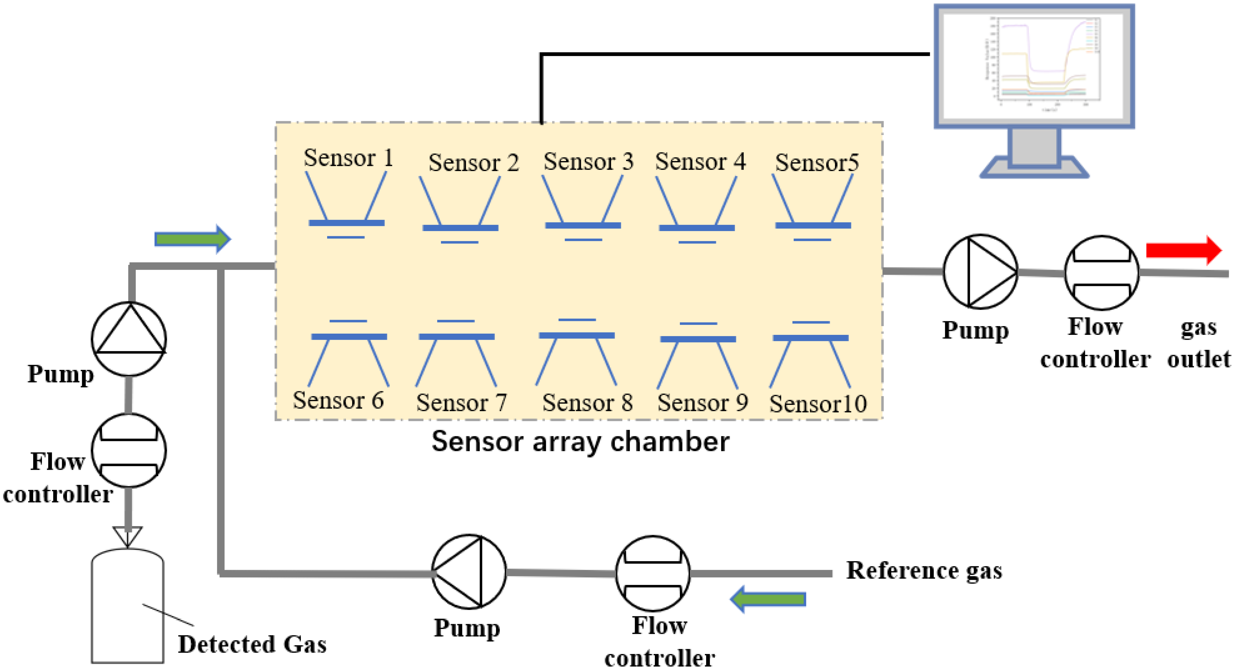
In order to verify the effectiveness of the as-proposed sensor array optimization model, we designed an E-nose system, as shown in Figure 1, which consists of three modules: sensor array (including 10 home-made MEMS metal oxide sensors), gas delivery module, and data acquisition module. The characteristics of the gas sensors in the initial sensor array are listed in Table 1.

Figure 1.
Schematic diagram of the experimental E-nose system.

Table 1.
Characteristics of the employed gas sensors in initial sensor array.
3.2. Experimental Procedures
In order to compare the recognition accuracy of the E-nose before and after the sensor array optimization, the above experimental system was used to identify the CO-CH4 gas mixtures. The compositions and concentrations of the gas samples are listed in Table 2. A total of 10 rounds of testing were carried out, and each round of testing included all types of gas mixtures, with the order of gas samples in each round of testing randomized. The temperature of the experimental environment was 25 ± 1 °C, and the humidity was 60 ± 5%. The data collection steps were as follows:
Table 2.
The composition and concentration of experimental gas samples.
- −
- Preheat the sensor array for 30 min, and flush the sensor array chamber with ambient air (300 mL/min) until the sensor baseline stabilizes.
- −
- Pump the target gas into the senser array chamber, the gas pumping time was 5 s and the response time was 120 s, and collect the response signal data of the sensor to the target gas during this whole process.
- −
- Purge the sensor array chamber with ambient air until all sensors return to their original baseline, then start the detection for the next gas sample.
4. Results
In this section, we firstly analyzed the responses of the as-designed E-nose to the CO-CH4 gas mixtures. Then, the sensor array optimization results of the selected four evaluation indicators and the proposed EWM-TOPSIS model were investigated, respectively, and the differences between them were compared. The obtained experimental results are as follows:
4.1. Response of the Initial Sensor Array to the Detected Gases
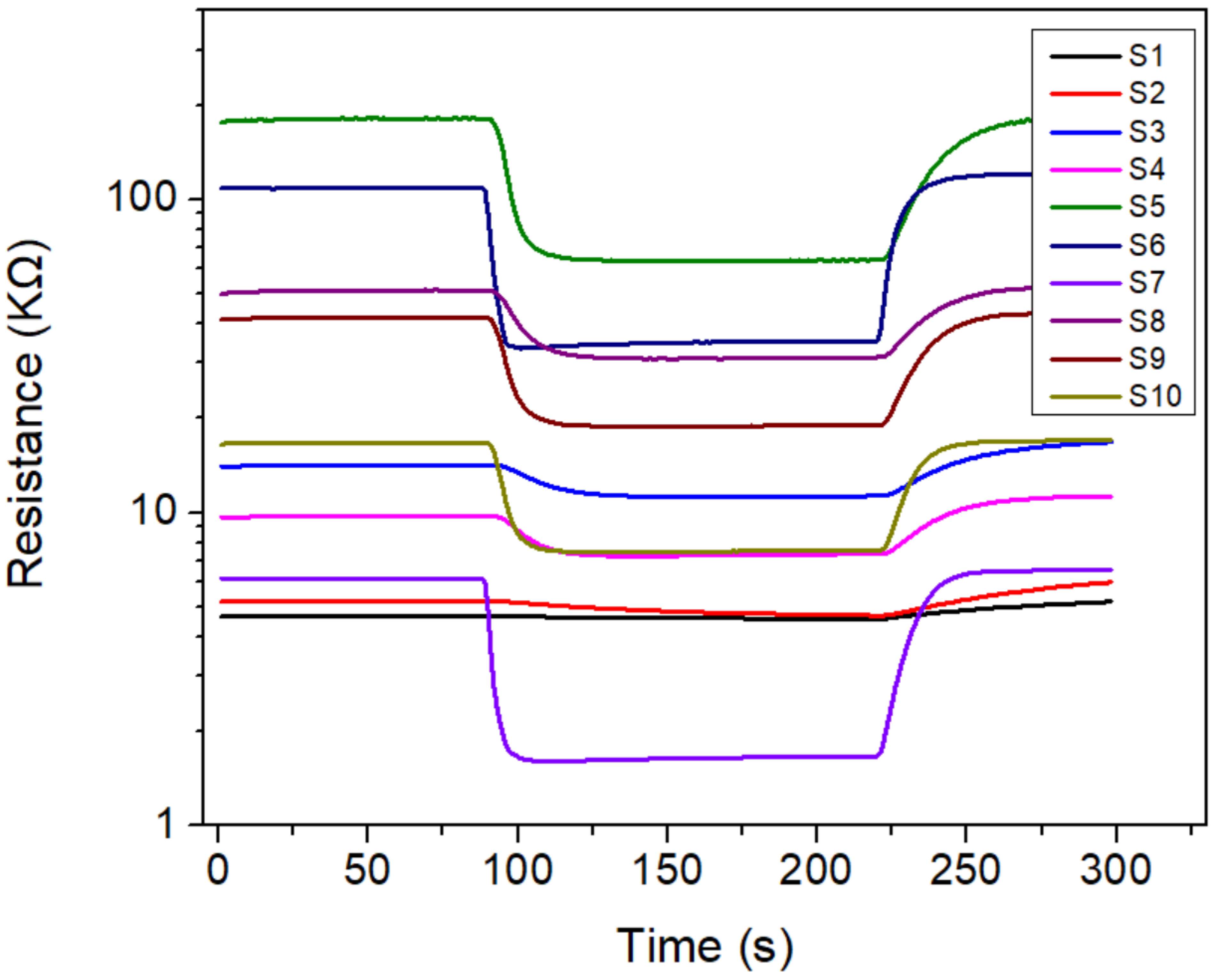
Figure 2 shows the typical response curves of the initial sensor array to CO-CH4 gas mixtures and each curve represents a different sensor’s transition with respect to detection time. It can be seen that although their initial resistances were different in the reference gas (ambient air), all of the sensors maintained stable baselines. When the CO-CH4 gas was introduced into the sensor array chamber, the resistances of all the sensors decreased sharply, and then reached a stable response state. After the target gas was pumped away, the sensor resistances gradually increased and returned to their baseline values. It can also be observed that the responses of different sensors to the CO-CH4 gas were significantly different. These results indicate that the as-designed E-nose had a good response to the target gas. However, although these sensors differed significantly in response to the target gas, it is still difficult to identify gases only from the response of a single sensor due to the inherent cross-sensitivity of the semiconductor sensors. Therefore, we could not tell which sensor has the possible optimal response with respect to the measured resistances before the E-nose optimization.
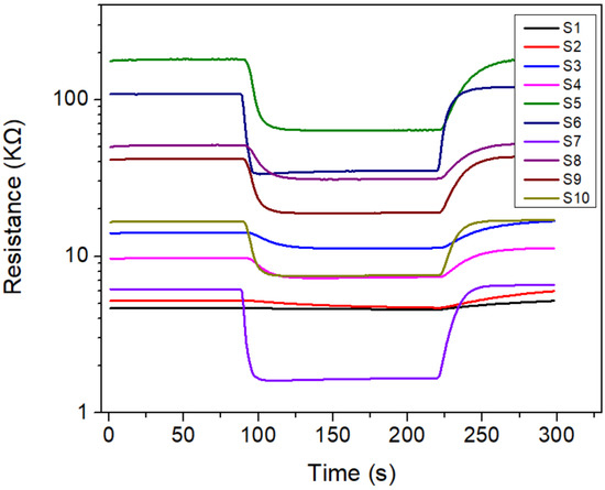
Figure 2.
Typical response curves of initial sensor array in CO-CH4 gas mixtures.
4.2. Analysis of Single Evaluation Indicator
4.2.1. Results of Sensitivity Indicator
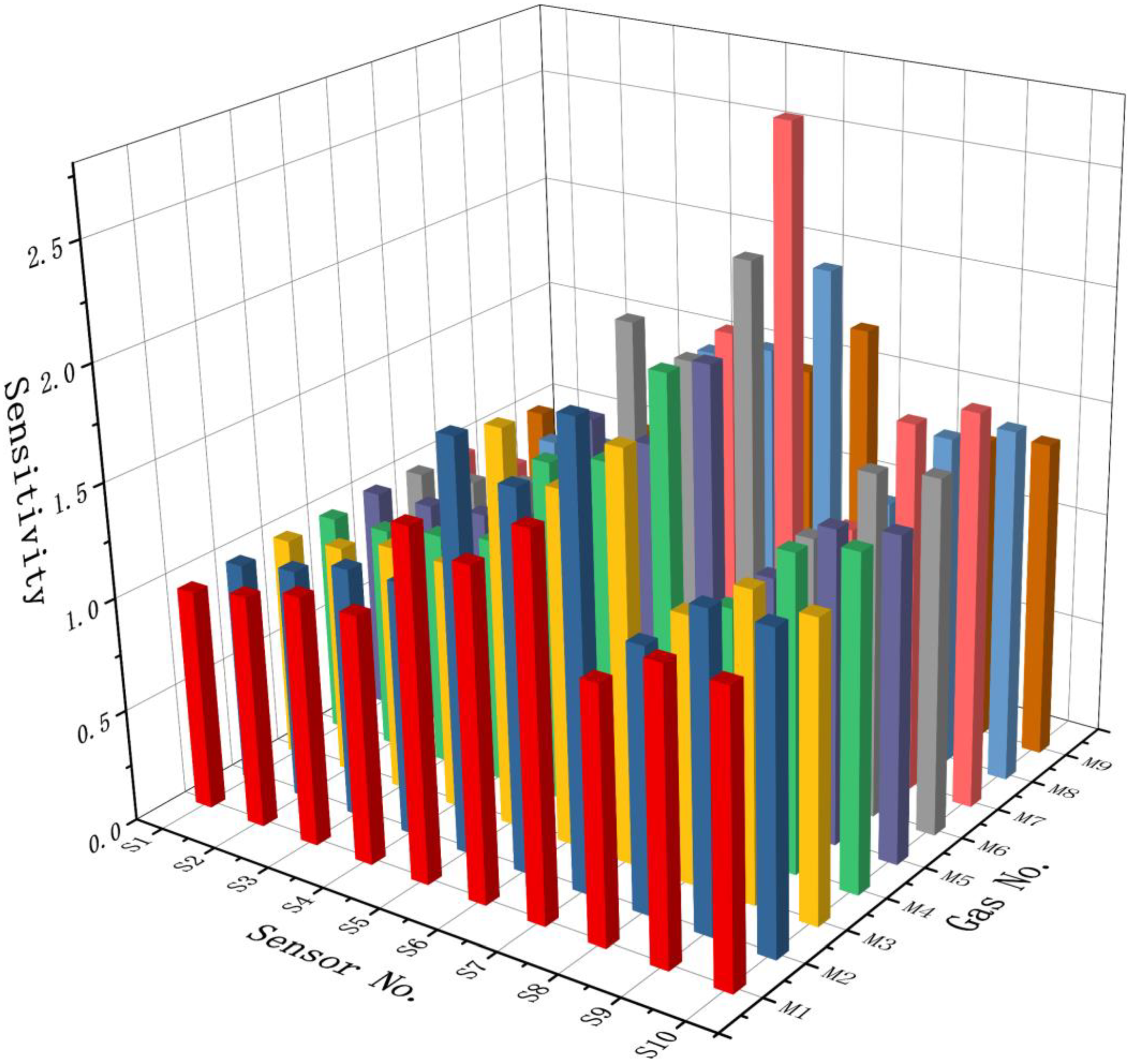
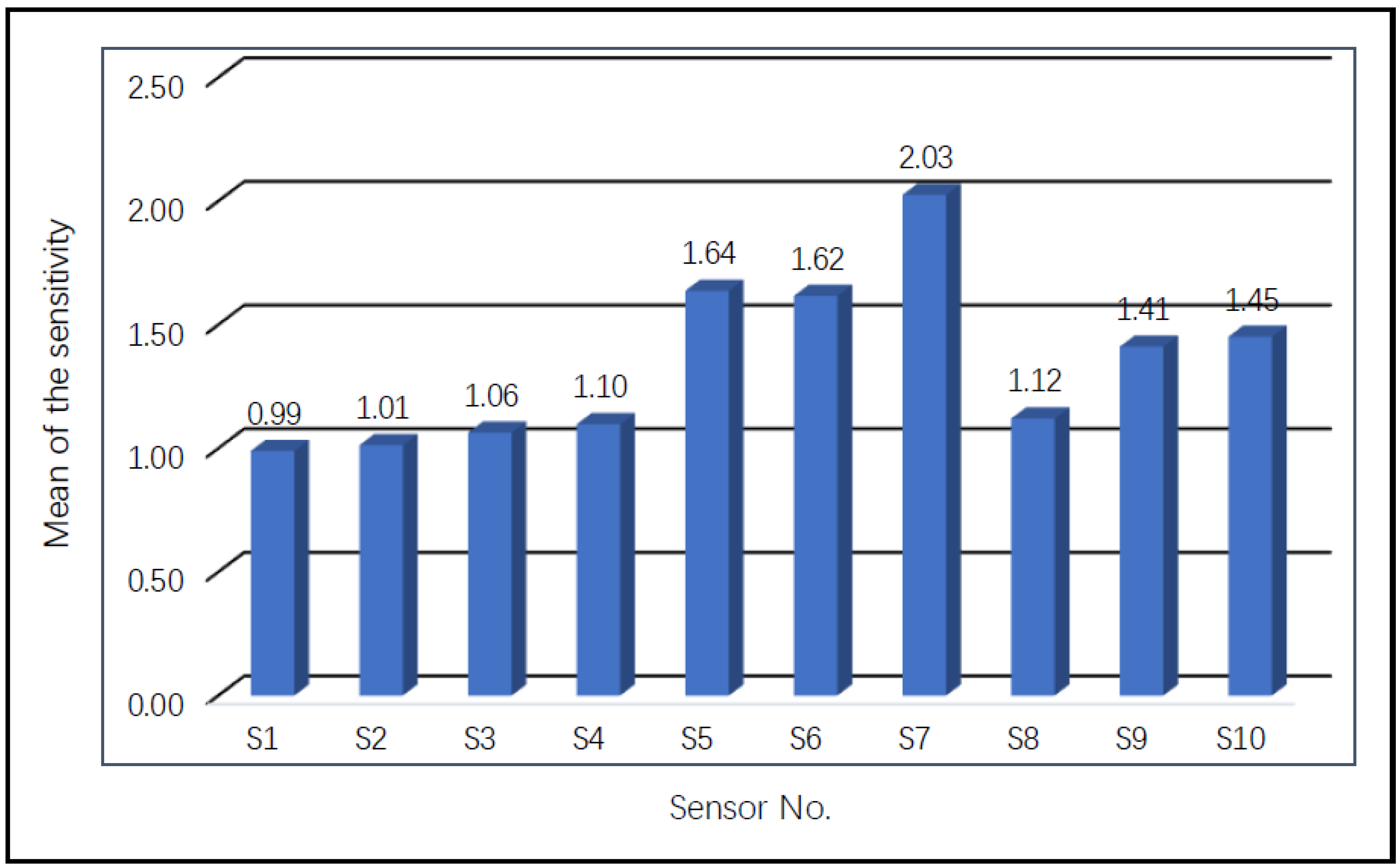
Figure 3 illustrates the sensitivities of all the sensors to the nine experimental gas mixtures, indicating that different sensors had obvious sensitivity differences to different gas samples. In order to observe the sensitivity of each sensor more intuitively, the average sensitivities of each sensor in all gas samples were calculated and are summarized in Figure 4. The three sensors with the highest average sensitivities were S7 (2.03), S5 (1.64), and S6 (1.62). In contrast, the three sensors with the lowest average sensitivities were S1 (0.99), S2 (1.01), and S3 (1.06). Therefore, from the perspective of sensitivity indicator, we removed sensors S1, S2, and S3 from the initial sensor array.

Figure 3.
Sensitivities of the initial sensor array to the experimental gas mixtures.
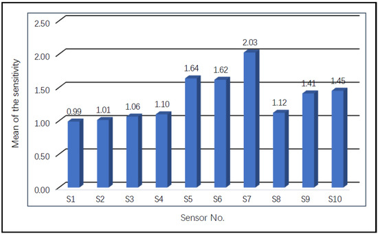
Figure 4.
Average sensitivities of different sensors to the experimental gas mixtures.
4.2.2. Results of Selectivity Indicator
Figure 5 shows the calculation results of the selectivity values of all the sensors to the experimental gases. Sensors S7 (4.14), S4 (1.63), and S9 (0.69) were the three sensors with the highest selectivity values, while sensors S1 (0.02), S2 (0.03), and S3 (0.06) performed the worst in the selectivity evaluation. From the sensitivity analysis results, the three sensors S1, S2, and S3 had poor abilities in distinguishing target gases, so they were eliminated from the initial sensor array.
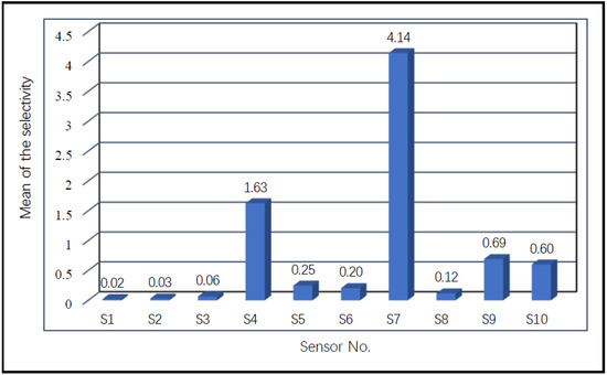
Figure 5.
Selectivity of the initial sensor array to the experimental gases.
4.2.3. Results of Correlation Indicator
The calculation result of the correlation evaluation between sensors is shown in Figure 6. It can be seen that there were high correlations between certain sensors, so the gas response data acquired by the initial sensor array may contain high information redundancy. For example, the correlation between sensors S6 and S7 was equal to 0.98. In order to reduce information redundancy and shorten calculation time, it may be considered to keep only one of the two sensors. Figure 7 shows the average value of the correlation coefficients between each sensor and the other 8 sensors. It can be observed from the calculation results that the three sensors with the smallest average correlation coefficients were S2 (0.69), S1 (0.71), and S6 (0.81), and the three sensors with the largest correlation coefficients were S8 (0.90), S9 (0.89), and S5 (0.89). A small correlation coefficient indicates that the sensor has less information redundancy with other sensors. From the perspective of improving the optimization performance of the sensor array, the sensors with small correlation coefficients were reserved. It should be noted that the pairwise correlation is more relevant than looking at the average correlations over all sensors. The average correlations were calculated just for observing the differences between sensors under the correlation evaluation indicator. Therefore, the comprehensive evaluation model proposed in this study is based on the pairwise sensor correlation.
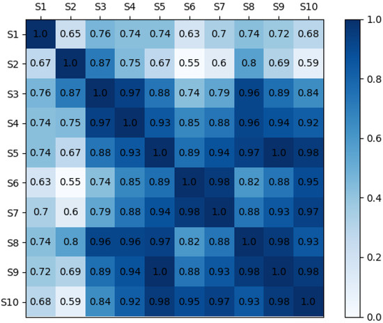
Figure 6.
Correlation coefficients between sensors in the initial sensor array.
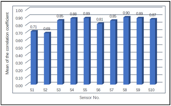
Figure 7.
The average value of the correlation coefficient between sensors.
4.2.4. Results of Repeatability Indicator
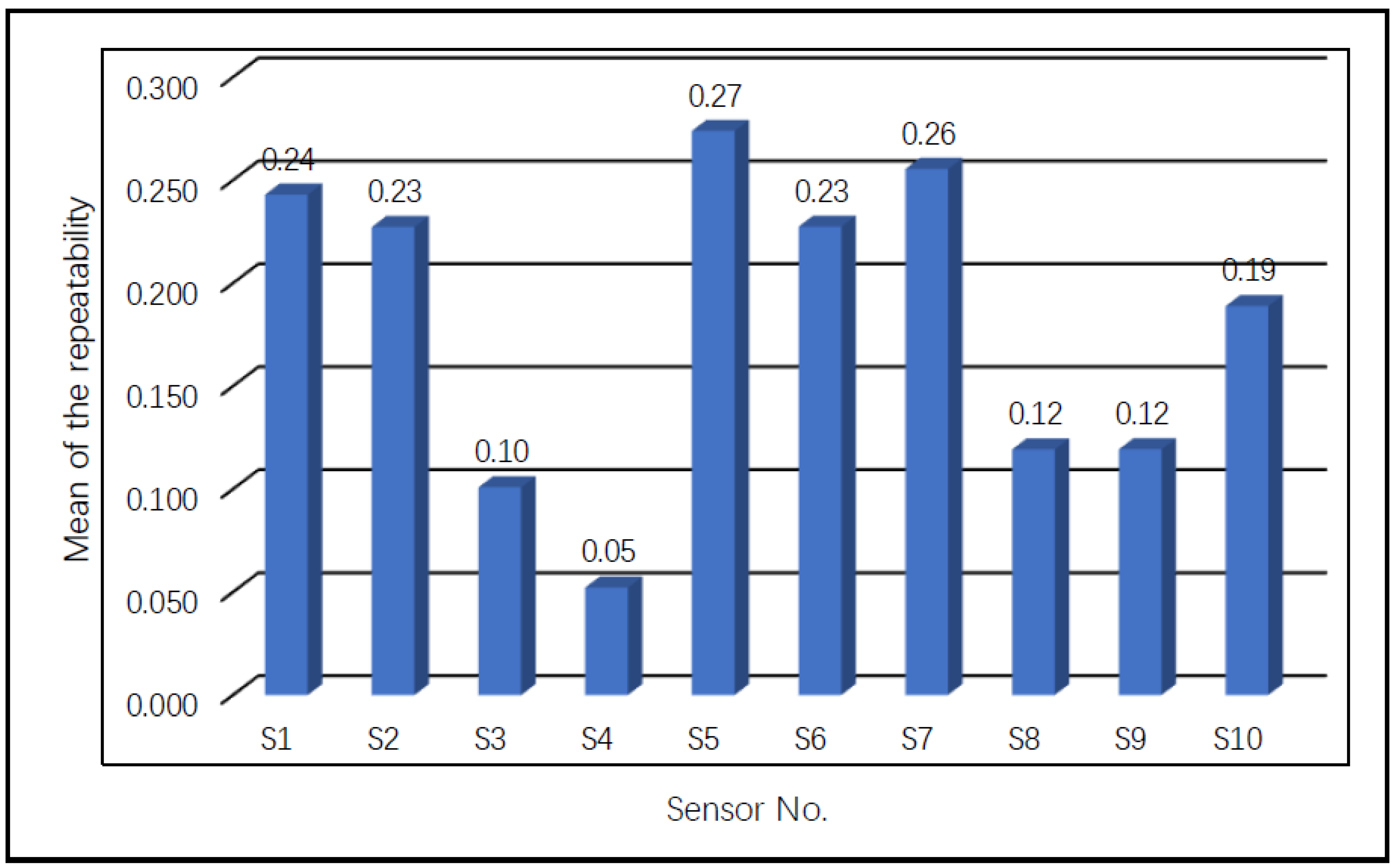
Figure 8 displays the repeatability results of all sensors to the experimental gases calculated according to Equation (4). The results confirmed that the repeatability values of different sensors in different gases were quite different. In order to compare the repeatability of each sensor, we calculated their average values (see Figure 9). It can be seen that the three sensors with the largest discrete values were S5 (0.27), S7 (0.26), and S1 (0.24), indicating that the experimental repeatability capabilities of these sensors were relatively low. In contrast, the three sensors with the smallest discrete values were S4 (0.05), S3 (0.1), and S8 (0.12). Therefore, in order to improve the stability of the E-nose performance, sensors S5, S7, and S1 were discarded from the initial sensing array.
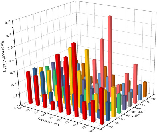
Figure 8.
Repeatability results of all sensors in the initial sensor array.
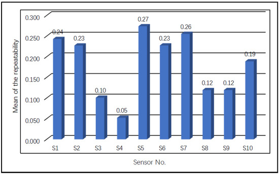
Figure 9.
The average values of the sensors’ repeatability evaluation results.
According to the analysis results of the four evaluation indicators, if the initial sensor array was optimized by removing the three sensors with the worst performances, the optimization results are summarized in Table 3. Both the sensitivity indicator and the selectivity indicator evaluated S1, S2, and S3 as the sensors with the worst performance, which indicates that there may be a certain correlation between the two evaluation indicators, that is, when a sensor has a low selectivity, its sensitivity may also be low. However, the correlation and repeatability evaluation results indicated a completely different situation. Therefore, according to these two evaluation indicators, deleting S5, S8, and S9, or S3, S4, and S8, respectively, can realize the optimization of the initial sensor array.
Table 3.
Optimization of the initial sensor array based on different evaluation indicators.
4.3. Weight Values of Evaluation Indicators
The above results analyzed each single evaluation indicator independently, so the optimization schemes obtained according to these indicators were different. Given that different evaluation indicators may have different impacts on the performance of the E-nose, it is not comprehensive to evaluate the sensor array only by a single evaluation indicator. Table 4 lists the weight value of each of the evaluation indicators calculated by EWM (Section 2.2). The weight value of the selectivity equaled 0.452, which was obviously higher than that of the other three indicators. This result indicates that selectivity was the most important among the four indicators. On the contrary, the correlation had the lowest weight value of 0.015. Therefore, it can be concluded that, compared with the other three indicators, the correlation had the least influence on the performance of the E-nose.
Table 4.
The weight values of the evaluation indicators calculated based on EWM.
4.4. Comprehensive Evaluation Results Based on the EWM-TOPSIS Model
Table 5 is the final evaluation score of the 10 sensors, calculated based on the EWM-TOPSIS model. The three sensors with the highest comprehensive evaluation scores were S7 (0.4232), S4 (0.2369), and S9 (0.091). The above experimental results have proved that the performances of these three sensors (S7, S4, and S9) were excellent for all single evaluation indicators. Therefore, it is reasonable that their comprehensive evaluation scores were also the highest. In contrast, the three sensors that obtained the lowest scores were S6 (0.028), S2 (0.007), and S1 (0.0052). According to the single indicator results, sensor S2 performed poorly in the evaluation of sensitivity and selectivity, and sensor S3 scored lower in the three indicators of sensitivity, selectivity, and repeatability. Although sensor S6 performed well in selectivity, it did not score highly in the repeatability evaluation. Their poor performances in the evaluation of different indicators makes their comprehensive evaluation scores lower. This result also proved the rationality of the as-proposed EWM-TOPSIS model. Therefore, according to the results of the comprehensive evaluation scores, we optimized the E-nose by removing sensors S1, S2, and S6 from the sensor array.
Table 5.
Evaluation scores of all sensors based on the EWM-TOPSIS model.
5. Discussion
5.1. Effect of Sensor Array Optimization on Extracted Gas Features
In order to verify the effect of sensor array optimization on the gas features extracted by the E-nose, we used the principal component analysis method (PCA) to analyze the experimental gas samples. The gas features for PCA were signal amplitudes collected on the nine types of gas mixtures using the as designed E-nose. Figure 10 shows the PCA analysis results—the contributions of PC1 and PC2 were 87.15% and 1.2%, respectively, and the total contribution of the two principal components equaled 88.35%, which indicates that the initial sensor array had the ability to sense different gases. However, the classification of the nine gas samples could not be discriminated because of the obvious overlap among many gas samples (gases M2, M3, M5, and M6, and the circles around individual groups in the figure were manually added as a guide for the eye). Therefore, the initial sensor array of the E-nose needs to be optimized.
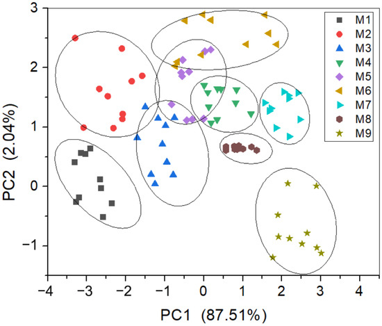
Figure 10.
PCA analysis of gas features extracted by E-nose with the initial sensor array.
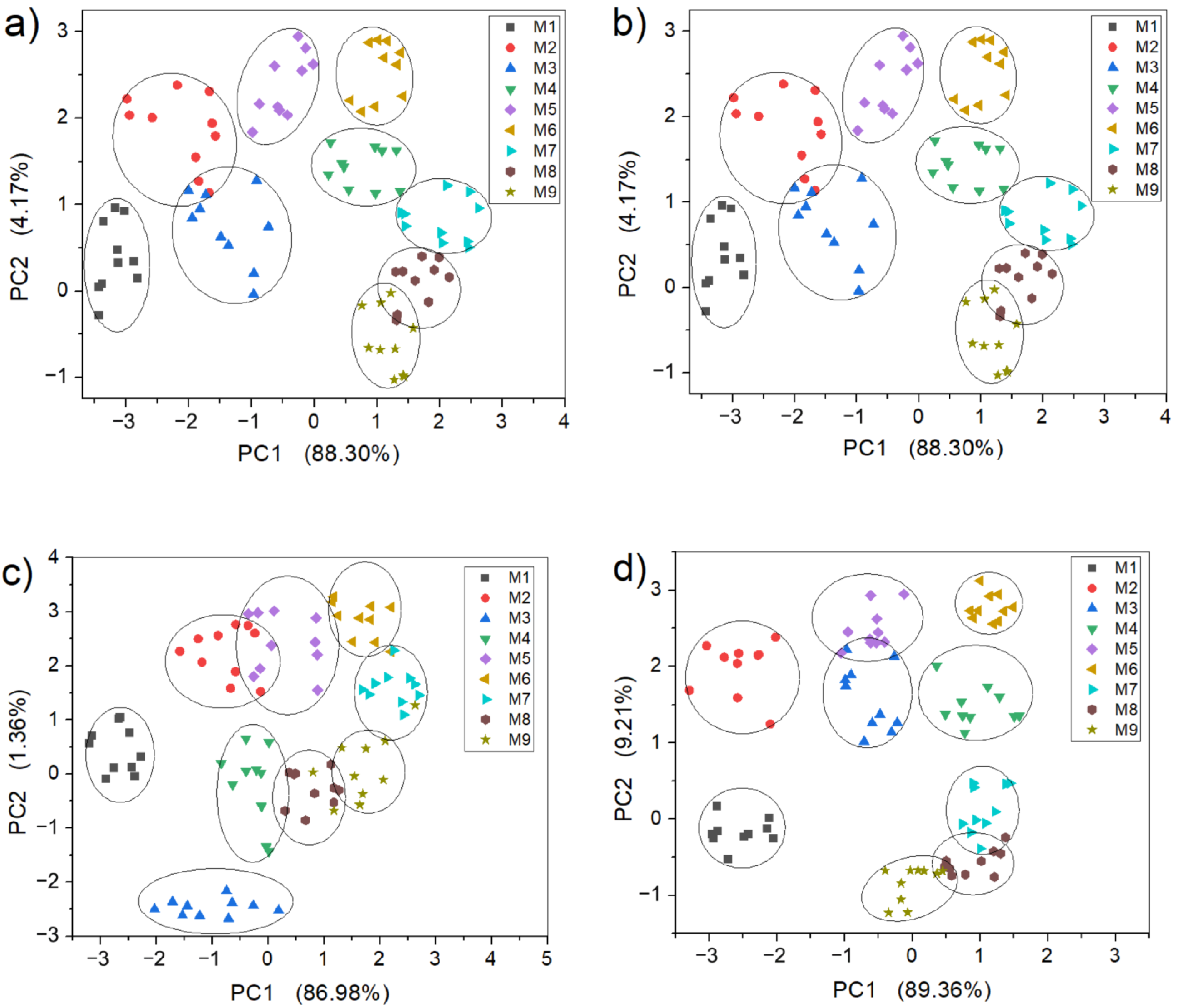
Figure 11 shows the PCA analysis results of the gas features extracted by E-nose, with the sensor array optimized according to different single evaluation indicators. After the sensitivity evaluation, the sensors S1, S2, and S3 were suggested to be removed from the initial sensor array, so the gas features were extracted based on the remaining seven sensors. According to the PCA result (Figure 11a), its two components of PC1 and PC2 explained 88.3% and 4.17% of the variance among the gas samples, respectively, and accounted for 92.47% of the total variance. The classification of gas samples was, therefore, improved compared with that of the initial sensor array, and the overlaps only existed between samples M2 and M3, and M8 and M9. Optimizing the sensing array according to the selectivity indicator yielded the same results as the sensitivity, given that the same sensors (S1, S2, and S3) were selected (see Figure 11b). The experimental results after removing sensors S5, S8, and S9 from the initial sensor array, in accordance with the correlation indicator, are shown in Figure 11c. It can be observed that except for samples M1 and M3, which were able to be completely separated, the rest of the samples still had partial overlap. However, compared with the initial sensing array, the discrimination of the rest of the samples was improved, which indicated that the sensors S5, S8, and S9 may have brought some redundant information, and removing them was beneficial for the E-nose to extract gas features. Figure 11d shows the experimental results of the sensor array optimized according to the repeatability indicator. It can be seen that the gas feature extraction ability of the optimized sensor array was also improved compared with the initial sensor array. It is worth noting that the sensor array optimized according to the correlation indicator was not as good as the sensitivity and selectivity indicators for gas feature extraction. According to the calculation results of the EWM, the weight value of the correlation indicator was the lowest among the four indicators. An evaluation indicator with a lower weight value inevitably has a weaker impact on the performance of the E-nose, so the optimization effect of the sensor array based on this indicator was poor. This result also proved the rationality of the weight value assignment based on the EWM proposed in this paper.
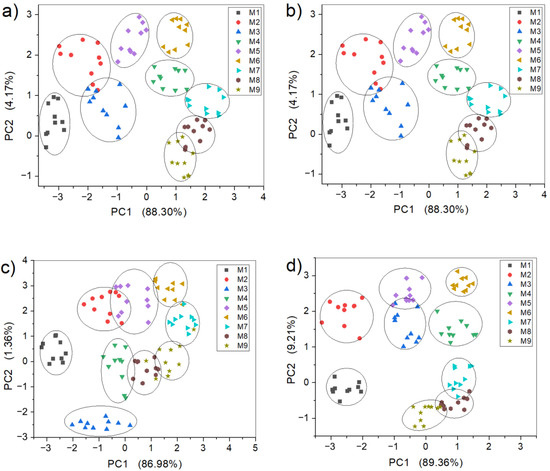
Figure 11.
PCA analysis of gas features extracted by E-nose with sensor array optimized based on a single evaluation indicator: (a) sensitivity, (b) selectivity, (c) correlation, and (d) repeatability.
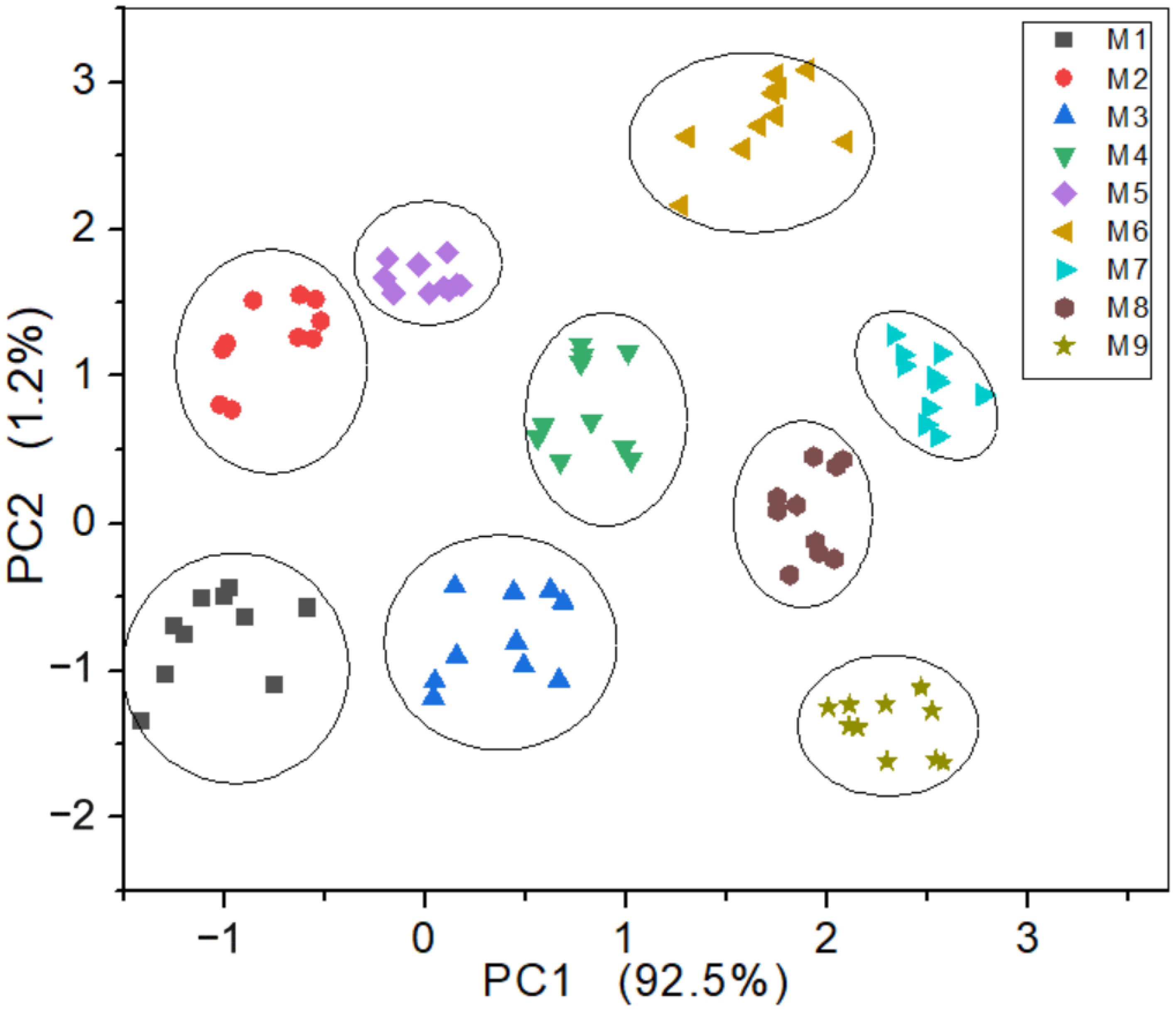
Although the ability of E-nose to extract gas features was improved after the sensor array optimization according to the four single evaluation indicators, there were still some samples that overlapped each other (see Figure 11). This is because a single evaluation indicator cannot achieve a comprehensive evaluation of the sensor array, so the sensor array has not been optimally optimized. Figure 12 shows the experimental results of the sensor array optimized by the EWM-TOPSIS model proposed in this paper. Its first component and second component could explain 92.5% and 1.2% of the variance among samples, respectively, and overall accounted for 93.7% of the total variance of data. It can be seen that the distinction of the extracted gas features was very obvious and there was no cross-overlapping phenomenon (as marked by the manually added circles in Figure 12). Compared with the optimization results of the single evaluation indicators, when sensor S6 was eliminated, the ability of the E-nose to extract gas features could be greatly improved. However, sensor S6 was not suggested to be removed from the initial sensor array by any single evaluation indicator. This result confirmed that the comprehensive evaluation of the sensor array cannot be achieved only by relying on the single evaluation indicators. Therefore, a comprehensive evaluation model is needed to comprehensively evaluate the sensor array and then realize its optimization.
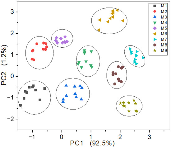
Figure 12.
PCA analysis of gas features extracted by the E-nose with the sensor array optimized based on EWM-TOPSIS model.
5.2. Effect of Sensor Array Optimization on Recognition Accuracy of E-nose
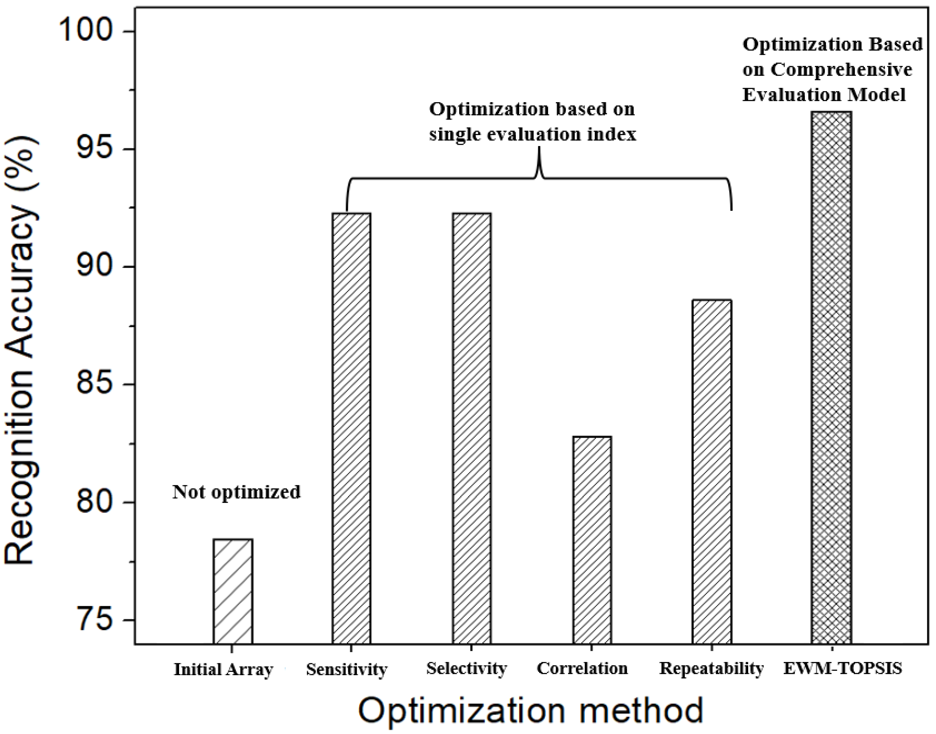
In order to investigate the influence of sensor array optimization on the recognition accuracy of the E-nose, this study established a gas recognition model using support vector machines (SVM), which selected RBF as the kernel function, and the hyperparameters C and gamma were determined through a network parametric search method. The experiment was carried out on the gas features extracted from the 90 CO-CH4 gas mixtures, in which 80% of the samples were randomly selected as the training dataset and 20% of the samples were used as the verification dataset, for which a fivefold cross-validation experiment was carried out. The classification accuracy of the nine mixed gases was taken as the recognition ability of the SVM model. Figure 13 shows the recognition accuracy before and after the sensor array optimization. It can be seen that after preliminary optimization based on the four single evaluation indicators, the highest recognition accuracy of the E-nose could reach to 93.3%, which was significantly improved compared with the 78.3% of the initial sensor array. After optimizing the sensor array through the EWM-TOPSIS model, the recognition accuracy of the electronic nose could be further improved to 96.5%. This proved that the comprehensive evaluation model could improve the recognition accuracy and was better than the single evaluation indicator in optimizing the sensor array for the E-nose.
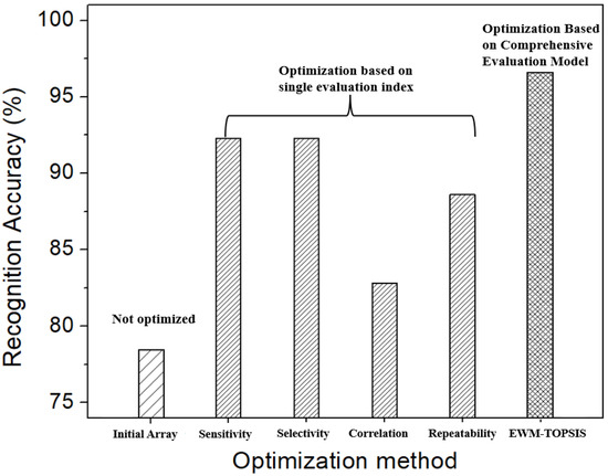
Figure 13.
Comparison of recognition accuracy of E-nose with different sensor array optimization methods.
6. Conclusions
In this paper, four evaluation indicators (sensitivity, selectivity, correlation, and repeatability) were selected to evaluate the sensor array in multiple dimensions, and a comprehensive evaluation model for sensor array optimization based on EWM-TOPSIS algorithm was proposed. In order to verify the effectiveness of the as-proposed model, it was applied to optimize the E-nose system containing 10 sensors, and a comparative investigation was carried out on the recognition ability of the E-nose with the sensor array before and after optimization. The main results are summarized as follows:
- (1)
- The optimization of the sensor array for E-nose according to a single evaluation indicator has limitations.
- (2)
- Different evaluation indicators contribute differently to the overall performance of the E-nose. Therefore, the weights of different evaluation indicators should be considered when comprehensively evaluating the sensor array.
- (3)
- The proposed comprehensive evaluation model based on EWM-TOPSIS can accurately reflect the contribution of different evaluation indicators to the overall performance of the sensor array, and the recognition accuracy of the E-nose with the sensor array optimized by this model can be significantly improved.
Author Contributions
Conceptualization, Y.Z. (Yongli Zhao); Methodology, Z.P. and Y.Z. (Yongli Zhao); Software, Z.P. and Y.Z. (Yongli Zhao); Validation, Z.P., Y.Z. (Yongli Zhao), J.Y., P.P., F.B., X.L., Y.G. and Q.R.; Formal analysis, Z.P. and Y.Z. (Yongli Zhao); Investigation, Y.Z. (Yongli Zhao), X.L., Y.G. and Q.R.; Resources, Y.Z. (Yongli Zhao); Data curation, J.Y., P.P., F.B. and Y.Z. (Yafei Zhang); Writing—original draft, Z.P. and Y.Z. (Yongli Zhao); Writing—review & editing, Y.Z. (Yongli Zhao); Visualization, Y.Z. (Yafei Zhang); Supervision, Y.Z. (Yongli Zhao); Project administration, Y.Z. (Yongli Zhao); Funding acquisition, Y.Z. (Yongli Zhao). All authors have read and agreed to the published version of the manuscript.
Funding
This research was supported by Major Special Science and Technology project of Anhui Province (No. 202103a07020007) and Key Research and Development Program of Anhui Province (No. 202104a05020057).
Institutional Review Board Statement
Not applicable.
Informed Consent Statement
Not applicable.
Data Availability Statement
Data is contained within the article.
Conflicts of Interest
The authors declare no conflict of interest.
References
- Ahmadipour, M.; Pang, A.L.; Ardani, M.R.; Pung, S.-Y.; Ooi, P.C.; Hamzah, A.A.; Wee, M.M.R.; Haniff, M.A.S.M.; Dee, C.F.; Mahmoudi, E.; et al. Detection of breath acetone by semiconductor metal oxide nanostructures-based gas sensors: A review. Mater. Sci. Semicond. Process. 2022, 149, 106897. [Google Scholar] [CrossRef]
- Cociorva, S.; Iftene, A. Indoor Air Quality Evaluation in Intelligent Building. Energy Procedia 2017, 112, 261–268. [Google Scholar] [CrossRef]
- Wen, J.; Zhao, Y.; Rong, Q.; Yang, Z.; Yin, J.; Peng, Z. Rapid odor recognition based on reliefF algorithm using electronic nose and its application in fruit identification and classification. J. Food Meas. Charact. 2022, 16, 2422–2433. [Google Scholar] [CrossRef]
- Wasilewski, T.; Gębicki, J. Emerging strategies for enhancing detection of explosives by artificial olfaction. Microchem. J. 2021, 164, 106025. [Google Scholar] [CrossRef]
- Feng, S.; Farha, F.; Li, Q.; Wan, Y.; Xu, Y.; Zhang, T.; Ning, H. Review on Smart Gas Sensing Technology. Sensors 2019, 19, 3760. [Google Scholar] [CrossRef]
- Bag, A.K.; Tudu, B.; Bhattacharyya, N.; Bandyopadhyay, R. Dealing with Redundant Features and Inconsistent Training Data in Electronic Nose: A Rough Set Based Approach. IEEE Sens. J. 2014, 14, 758–767. [Google Scholar] [CrossRef]
- Cheng, L.; Meng, Q.-H.; Lilienthal, A.J.; Qi, P.-F. Development of compact electronic noses: A review. Meas. Sci. Technol. 2021, 32, 062002. [Google Scholar] [CrossRef]
- Alizadeh, T. Chemiresistor sensors array optimization by using the method of coupled statistical techniques and its application as an electronic nose for some organic vapors recognition. Sens. Actuators B Chem. 2010, 143, 740–749. [Google Scholar] [CrossRef]
- Yin, Y.; Yu, H.; Chu, B.; Xiao, Y. A sensor array optimization method of electronic nose based on elimination transform of Wilks statistic for discrimination of three kinds of vinegars. J. Food Eng. 2014, 127, 43–48. [Google Scholar] [CrossRef]
- Xu, Z.; Shi, X.; Lu, S. Integrated sensor array optimization with statistical evaluation. Sens. Actuators B Chem. 2010, 149, 239–244. [Google Scholar] [CrossRef]
- Leccese, F.; Cagnetti, M.; Giarnetti, S.; Petritoli, E.; Tuti, S.; Luisetto, I.; Pecora, A.; Maiolo, L.; Durovic-Pejcev, R.; Dordevic, T.; et al. Electronic Nose: A First Sensors Array Optimization for Pesticides Detection Based on Wilks’ A-Statistic. In Proceedings of the 2018 5th IEEE International Workshop on Metrology for AeroSpace (MetroAeroSpace), Rome, Italy, 20–22 June 2018. [Google Scholar]
- Chen, R.R.; Luo, D.H.; Sun, Y.; Sun, Y.L.; Hossini, H.G. A Sensor Array Optimization Method Based on Variance Difference for Machine Olfaction. Appl. Mech. Mater. 2014, 618, 523–527. [Google Scholar] [CrossRef]
- Borowik, P.; Adamowicz, L.; Tarakowski, R.; Siwek, K.; Grzywacz, T. Odor Detection Using an E-Nose with a Reduced Sensor Array. Sensors 2020, 20, 3542. [Google Scholar] [CrossRef]
- Chaudry, A.N.; Hawkins, T.; Travers, P. A method for selecting an optimum sensor array. Sens. Actuators B Chem. 2000, 69, 236–242. [Google Scholar] [CrossRef]
- Russo, R.D.F.S.M.; Camanho, R. Criteria in AHP: A Systematic Review of Literature. Procedia Comput. Sci. 2015, 55, 1123–1132. [Google Scholar] [CrossRef]
- Zhu, Y.; Tian, D.; Yan, F. Effectiveness of Entropy Weight Method in Decision-Making. Math. Probl. Eng. 2020, 2020, 3564835. [Google Scholar] [CrossRef]
- Yu, L.; Yang, W.; Duan, Y.; Long, X. A Study on the Application of Coordinated TOPSIS in Evaluation of Robotics Academic Journals. Math. Probl. Eng. 2018, 2018, 5456064. [Google Scholar] [CrossRef]
- Zhao, C.; Zhao, Y. The investigation of Zn content on the structure and electrical properties of ZnxCu0.2Ni0.66Mn2.14−xO4 negative temperature coefficient ceramics. J. Mater. Sci. Mater. Electron. 2012, 23, 1788–1792. [Google Scholar] [CrossRef]
- Tong, Y.; Zhao, B.; Zhao, Y.; Yang, T.; Yang, F.; Hu, Q.; Zhao, C. Novel Anode-Supported Tubular Solid-Oxide Electrolytic Cell for Direct NO Decomposition in N2 Environment. Int. J. Electrochem. Sci. 2015, 10, 5338–5349. [Google Scholar]
- Zhao, Y.; Zhao, C.; Huang, J.; Zhao, B. LaMnO3–Ni0.75Mn2.25O4 Supported Bilayer NTC Thermistors. J. Am. Ceram. Soc. 2014, 97, 1016–1019. [Google Scholar] [CrossRef]
- Zhao, Y.; Zhao, C.; Tong, Y. Spinel-structured Ni-free Zn0.9CuxMn2.1−xO4 (0.1 ≤ x ≤ 0.5) thermistors of negative temperature coefficient. J. Electroceramics 2013, 31, 286–290. [Google Scholar] [CrossRef]
- Kumar, R.; Singh, S.; Bilga, P.S.; Jatin; Singh, J.; Singh, S.; Scutaru, M.-L.; Pruncu, C.I. Revealing the benefits of entropy weights method for multi-objective optimization in machining operations: A critical review. J. Mater. Res. Technol. 2021, 10, 1471–1492. [Google Scholar] [CrossRef]
- Salih, M.M.; Zaidan, B.; Zaidan, A.; Ahmed, M.A. Survey on fuzzy TOPSIS state-of-the-art between 2007 and 2017. Comput. Oper. Res. 2019, 104, 207–227. [Google Scholar] [CrossRef]


Disclaimer/Publisher’s Note: The statements, opinions and data contained in all publications are solely those of the individual author(s) and contributor(s) and not of MDPI and/or the editor(s). MDPI and/or the editor(s) disclaim responsibility for any injury to people or property resulting from any ideas, methods, instructions or products referred to in the content. |
© 2023 by the authors. Licensee MDPI, Basel, Switzerland. This article is an open access article distributed under the terms and conditions of the Creative Commons Attribution (CC BY) license (https://creativecommons.org/licenses/by/4.0/).