Kernel Learning by Spectral Representation and Gaussian Mixtures

Abstract

One of the main tasks in kernel methods is the selection of adequate mappings into higher dimension in order to improve class classification. However, this tends to be time consuming, and it may not finish with the best separation between classes. Therefore, there is a need for better methods that are able to extract distance and class separation from data. This work presents a novel approach for learning such mappings by using locally stationary kernels, spectral representations and Gaussian mixtures.

1. Introduction

During the 90’s, the use of kernels [1,2,3,4,5] in Machine Learning received a considerable attention for their ability to improve the performance of linear classifiers. By using kernels, Support Vector Machines and other kernel methods [6,7] can classify complex data sets by mapping them into high dimensional spaces. However, an underlying issue exists, summarized by a simple question: Which kernel should be used? [8].

Kernel selection is not a small task and would highly depend on the problem to be solved. A first idea to select the best kernel could be evaluating different kernels from a small set using leave-one-out cross-validation and selecting the kernel with better classification properties. Nevertheless, this can become a time-consuming task when the number of samples range in the thousands. A better idea is to use a combination of kernels to create kernels with better classification properties. Methods using this type of techniques are called Multiple Kernel Learning (MKL) [9]. For example, Lanckriet [10] uses a Semi-Definite Programming (SDP) to find the best conic combination of multiple kernels. However, these methods still require some pre-selected set of kernels as inputs. A better plan will be to use the distance information at the class data sets. For example, Hoi [11] tries to find a kernel Gram matrix by building the Laplacian Graph [12] of the data. Then, an SDP is applied to find the best combination of kernels.

However, none of these methods are scalable given that their Gram matrix needs to be built the computational complexity of building a Gram matrix is $(O\left(N^2\right)$ where N is the number of samples. As a possible solution, it has been proposed to use Sequential Minimal Optimization (SMO) [13] to reduce complexity. This allows to move the quadratic programming problem to a quadratic programming sub-problems. For example, Bach [14] uses an SDP setup and solves the problem by using an SMO algorithm. Other techniques [15] use a random sample of the training set, and a possible approximation to the Gram Matrix to reduce complexity $(O(m^{2}N+m^2+mN)$, m sub-problem size). Expanding on this idea, Rahimi [16] approximates kernel functions using samples of the distribution, but only for stationary kernels. On the other hand, Ghiasi-Shirazi [17] proposes a method for learning m number of stationary kernels in the approach of MKL. The method has a main advantage, its ability to learn m number of kernels in an unsupervised way by reducing the complexity of the output function. Furthermore, it reduces the complexity of the classifier output from $O\left(mxNx{N}_{S}V\right)$ to $O\left(mxN\right)$ by using m kernels. Finally, Oliva [18], makes use of Bayesian methods to learn a stationary kernel in a non-parametric way.

On this work, we propose to learn locally stationary kernel from data, given that stationary kernels are a subset of the locally stationary kernel, by using a spectral representation and Gaussian Mixtures [19]. This allows to improve the classification and regression task by looking at the kernel as the result of a sampling process on a spectral representation. This paper is structured in the following way: in Section 2, we show the basic theory to understand the idea of stationary and locally stationary kernels. In Section 3, the proposed algorithm is developed by using Fourier Basis and sampling. Additionally, a theorem is given about the performance of the spectral representation. In Section 4, we review the experiments for classification and regression tasks to test the robustness of the proposed algorithm. Finally, we present an analysis of the advantages of the proposed algorithm and possible venues of research in the Section 5.

2. The Concept of Kernels

The main idea of using kernel methods is to obtain the distance between samples on higher dimensional. Thus, avoid mapping the samples to higher dimensional spaces and using the inner product for such process. In other words, let $\mathcal{X}\subseteq {\mathbb{R}}^D$ be the input set, where $D\in \mathbb{N}$, let $\mathcal{K}$ be a feature space, and suppose the feature mapping function is defined as $\mathit{\phi }:\mathcal{X}\to \mathcal{K}$. Hence, the kernel function, $\kappa :\mathcal{X}\times \mathcal{X}\to \mathbb{R}$, has the following property:

$$\kappa (\mathit{x},{\mathit{x}}^{\prime })\equiv ⟨\mathit{\phi }\left(\mathit{x}\right),\mathit{\phi }\left({\mathit{x}}^{\prime }\right)⟩,$$

where $\mathit{x},{\mathit{x}}^{\prime }\in \mathcal{X}$. Thus, $\mathit{\phi }$ and the feature space can be implicitly defined. Now, let ${\left\{{\mathit{x}}_i\right\}}_{i=1}^N$ be the set of samples, $\kappa :\mathcal{X}\times \mathcal{X}\to \mathbb{R}$ be a valid kernel, and $⟨·,·⟩$ be a well defined inner product. Then, the elements at the Gram Matrix, $K\in {\mathbb{R}}^{N\times N}$, are computed using the $\kappa$ mapping, $K_{ij}:=\kappa ({\mathit{x}}_i,{\mathit{x}}_j)$. Given this definition, Genton [20] makes an in-depth study of the class of kernel from a statistics perspective, i.e., the kernel functions as a co-variance function. He pointed out that kernels have a spectral representation which can be used to represent their Gram matrix. Based on this representation, the proposed algorithm learns the Gram matrix by using a Gibbs sampler to obtain the structure of such matrix.

2.1. Stationary Kernels

Stationary kernels [20] are defined as $\kappa (\mathit{x},{\mathit{x}}^{\prime })={\kappa }_s(\mathit{x}-{\mathit{x}}^{\prime })$. An important factor in such definition is its dependency on the lag vector which can be interpreted as generalizations of the Gaussian probability distribution functions which are used to represent distributions [15]. Additionally, Bochner [21] proved that a symmetric function ${\kappa }_s$ is a positive definite in ${\mathbb{R}}^D$, if and only if, it has the form:

$${\kappa }_s(\mathit{x}-{\mathit{x}}^{\prime })={\int }_{{\mathbb{R}}^D}{e}^{2\pi i{\mathit{\omega }}^T(\mathit{x}-{\mathit{x}}^{\prime })}d\mu (\mathit{\omega }),$$

(1)

where $\mu$ is a positive finite measure. Equation (1) is called the spectral representation of ${\kappa }_s$. Now, suppose $\mu$ has a density $F(\mathit{\omega })$ and $\mathit{\tau }=\mathit{x}-{\mathit{x}}^{\prime }$. Thus, it is possible to obtain:

$$\begin{array}{cc}\hfill \kappa (\mathit{\tau })& =\int F(\mathit{\omega })e^{2\pi i{\mathit{\omega }}^T\mathit{\tau }}d\mathit{\omega },\hfill \\ \hfill F(\mathit{\omega })& =\int \kappa (\mathit{\tau })e^{-2\pi i{\mathit{\omega }}^T\mathit{\tau }}d(\mathit{\tau }).\hfill \end{array}$$

In other words, the kernel function ${\kappa }_s$ and its spectral density F are Fourier dual of each other. Furthermore, if $\kappa \left(\mathbf{0}\right)=\int F(\mathit{\omega })d\mathit{\omega }$ and F is a probability measure, the unique condition to define a valid Gaussian process is $\kappa \left(\mathbf{0}\right)=1$. In other words, we need this condition to ensure that the kernel $\kappa$ and the function f are correctly correlated.

2.2. Locally Stationary Kernels

Extending on the previous concept, Silverman [22] defines the locally stationary kernels as:

$$\kappa (\mathit{x},\mathit{x}):={\kappa }_1\left(\frac{\mathit{x}+{\mathit{x}}^{\prime }}{2}\right){\kappa }_s(\mathit{x}-{\mathit{x}}^{\prime }),$$

(2)

where ${\kappa }_1$ is a non negative function and ${\kappa }_s$ is a stationary kernel. This type of kernels increase the power of the representation by introducing a possible variance into the final calculated similarity through the use of ${\kappa }_1$. Furthermore, we can see from Equation (2) that the Locally Stationary Kernels include all stationary kernels. In order to see this, we make ${\kappa }_1(·)=c$, where c is a positive constant, then $\kappa (\mathit{x},\mathit{x}):=c{\kappa }_s(\mathit{x}-{\mathit{x}}^{\prime })$, a multiple of all stationary kernels. Furthermore, the variance of locally stationary kernels is given by $\mathit{x}={\mathit{x}}^{\prime }$, thus, the variance is defined as:

$$\kappa (\mathit{x},\mathit{x})=\kappa \left(\mathit{x}\right)\kappa \left(\mathbf{0}\right)={\kappa }_1\left(\mathit{x}\right),$$

This means that the variance of the Locally Stationary Kernels relies in the positive definite function ${\kappa }_1$.

The spectral representation of a locally stationary kernel is also given by [22], and it is defined as:

$${\kappa }_1\left(\frac{\mathit{x}+{\mathit{x}}^{\prime }}{2}\right){\kappa }_s(\mathit{x}-{\mathit{x}}^{\prime })={\int }_{\mathcal{X}}{\int }_{\mathcal{X}}exp\left(i\frac{{\mathit{\omega }}_1^T\mathit{x}-{\mathit{\omega }}_2^T{\mathit{x}}^{\prime }}{2}\right)f_1\left(\frac{{\mathit{\omega }}_1+{\mathit{\omega }}_2}{2}\right)f_2({\mathit{\omega }}_1-{\mathit{\omega }}_2)d{\mathit{\omega }}_{1}d{\mathit{\omega }}_2.$$

Furthermore, by setting $\mathit{x}={\mathit{x}}^{\prime }=\mathbf{0}$, we can get:

$$\kappa (\mathbf{0},\mathbf{0})={\int }_{\mathcal{X}}{\int }_{\mathcal{X}}{f}_1\left(\frac{{\mathit{\omega }}_1+{\mathit{\omega }}_2}{2}\right)f_2({\mathit{\omega }}_1-{\mathit{\omega }}_2)d{\mathit{\omega }}_{1}d{\mathit{\omega }}_2.$$

Consequently, in order to define a locally stationary kernel, $f_1$ and $f_2$ must be integrable functions. Additionally, an important fact is that the kernel $\kappa$ has a defined inverse, given by:

$$f_1\left(\frac{{\mathit{\omega }}_1+{\mathit{\omega }}_2}{2}\right)f_2({\mathit{\omega }}_1-{\mathit{\omega }}_2)=\frac{1}{{\left(2\pi \right)}^2}{\int }_{\mathcal{X}}{\int }_{\mathcal{X}}{\kappa }_1\left(\frac{{\mathit{x}}_1+{\mathit{x}}^{\prime }}{2}\right){\kappa }_2(\mathit{x}-{\mathit{x}}^{\prime })d\mathit{x}d{\mathit{x}}^{\prime }.$$

Moreover, $f_2$ is the Fourier transform of ${\kappa }_1$ and $f_1$ is the Fourier transform of ${\kappa }_2$. Thus, if we introduce two dummy variables $\mathit{u}=(\mathit{x}+{\mathit{x}}^{\prime })/2$ and $\mathit{v}=\mathit{x}-{\mathit{x}}^{\prime }$, it is possible to obtain:

$$\begin{array}{cc}\hfill f_1\left({\mathit{\omega }}_1\right)& =\frac{1}{2\pi }{\int }_{\mathcal{X}}exp(-i{\mathit{v}}^T{\mathit{\omega }}_1){\kappa }_2\left(\mathit{v}\right)d\mathit{v}\hfill \\ \hfill f_2\left({\mathit{\omega }}_2\right)& =\frac{1}{2\pi }{\int }_{\mathcal{X}}exp(-i{\mathit{u}}^T{\mathit{\omega }}_2){\kappa }_1\left(\mathit{u}\right)d\mathit{u}\hfill \end{array}$$

and

$$\begin{array}{cc}\hfill {\kappa }_1\left(\mathit{u}\right)& ={\int }_{\mathcal{X}}exp\left(i{\mathit{u}}^T{\mathit{\omega }}_2\right)f_2\left({\mathit{\omega }}_2\right)d{\mathit{\omega }}_2\hfill \\ \hfill {\kappa }_2\left(\mathit{v}\right)& ={\int }_{\mathcal{X}}exp\left(i{\mathit{v}}^T{\mathit{\omega }}_1\right)f_1\left({\mathit{\omega }}_1\right)d{\mathit{\omega }}_1,\hfill \end{array}$$

with this in mind, it is possible to use the ideas in [16] to approximate the locally stationary kernels.

3. Approximating Stationary Kernels

Rahimi [16] makes use of (1) to approximate stationary kernels. This is, if we define ${\zeta }_{\mathit{\omega }}=exp\left(i{\mathit{\omega }}^T\mathit{x}\right)$; then, Equation (1) becomes:

$$\kappa (\mathit{x}-{\mathit{x}}^{\prime })={\int }_{\mathcal{X}}f(\mathit{\omega })exp\left(i{\mathit{\omega }}^T(\mathit{x}-{\mathit{x}}^{\prime })\right)d\mathit{\omega }={\mathbb{E}}_{\mathit{\omega }}\left[{\zeta }_{\mathit{\omega }}\left(\mathit{x}\right){\zeta }_{\mathit{\omega }}^{*}\left({\mathit{x}}^{\prime }\right)\right]$$

where $\mathit{\omega }\sim f$. Now, using Monte Carlo integration and taking ${\mathit{\omega }}_j\sim f$, the kernel can be approximated as

$$\kappa (\mathit{x}-{\mathit{x}}^{\prime })\approx \frac{1}{M_1}\sum _{j=1}^{M_1}{\zeta }_{{\omega }_j}\left(\mathit{x}\right){\zeta }_{{\omega }_j}^{*}\left({\mathit{x}}^{\prime }\right).$$

(3)

In particular, if the kernel is real-valued; then, Equation (3) becomes

$$\kappa (\mathit{x}-{\mathit{x}}^{\prime })\approx \frac{1}{M_1}{\mathit{\varphi }}^T\left(\mathit{x}\right)\mathit{\varphi }\left({\mathit{x}}^{\prime }\right),$$

(4)

where $\mathit{\varphi }\left(\mathit{s}\right)=[cos({\mathit{\omega }}_1^T\mathit{s}),\dots ,cos({\mathit{\omega }}_{M_1}^T\mathit{s}),sin({\mathit{\omega }}_1^T\mathit{s}),\dots ,sin({\mathit{\omega }}_{M_1}^T\mathit{s})]$. A side effect of (4) is that we can compute $f\left(\mathit{x}\right)$ as $f\left(\mathit{x}\right)={\sum }_{i=1}^n{\alpha }_i\kappa ({\mathit{x}}_i-\mathit{x})$. This means that function f can be approximated as

$$f\left(\mathit{x}\right)\approx \frac{1}{M}\sum _{i=1}^n{\alpha }_i\mathit{\varphi }{\left({\mathit{x}}_i\right)}^T\mathit{\varphi }\left(\mathit{x}\right)={\gamma }^T\mathit{\varphi }\left(\mathit{x}\right)$$

where $\gamma =\frac{1}{M}{\sum }_{i=1}^n{\alpha }_i\mathit{\varphi }\left({\mathit{x}}_i\right)$ is a constant. This constant makes possible to avoid some of the operations to obtain the Gram matrix.

3.1. Approximating Locally Stationary Kernel

As we know, ${\kappa }_2$ is a stationary kernel which allows to approximate ${\kappa }_2$ as presented in Section 3. Now, to obtain the locally stationary kernel, we would like to approximate ${\kappa }_1$. For this, we define ${\zeta }_{\mathit{v}}^{\prime }\left(\mathit{x}\right)=exp(i{\mathit{v}}^T\mathit{x}/2)$:

$${\kappa }_1\left(\frac{\mathit{x}+{\mathit{x}}^{\prime }}{2}\right)={\int }_{{\mathbb{R}}^D}exp\left(i{\mathit{v}}^T\left(\frac{\mathit{x}+{\mathit{x}}^{\prime }}{2}\right)\right)f_2\left(\mathit{v}\right)d\mathit{v}={\mathbb{E}}_{\mathit{v}}\left[{\zeta }_{\mathit{v}}^{\prime }\left(\mathit{x}\right){\zeta }_{\mathit{v}}^{\prime }\left(\mathit{x}\right)\right],$$

where $\mathit{v}\sim f_2$. Using Monte Carlo integration and taking ${\mathit{v}}_k\sim f_2$, for $k=1,2,\dots ,M_2$, it is possible to approximate ${\kappa }_1$ as:

$${\kappa }_1\left(\frac{\mathit{x}+{\mathit{x}}^{\prime }}{2}\right)\approx \frac{1}{M_2}\sum _{k=1}^{M_2}{\zeta }_{{\mathit{v}}_k}^{\prime }\left(\mathit{x}\right){\zeta }_{{\mathit{v}}_k}^{\prime }\left({\mathit{x}}^{\prime }\right).$$

(5)

To approximate the output of the locally stationary kernel, we can use Equations (3) and (5) as follows:

$$\begin{array}{cc}\hfill \kappa (\mathit{x},{\mathit{x}}^{\prime })& ={\kappa }_1\left(\frac{\mathit{x}+{\mathit{x}}^{\prime }}{2}\right){\kappa }_2(\mathit{x}-{\mathit{x}}^{\prime })\hfill \\ \hfill & \approx \frac{1}{M_1{M}_2}\left(\sum _{k=1}^{M_2}exp\left(i\frac{{\mathit{v}}_k^T\mathit{x}}{2}\right)exp\left(i\frac{{\mathit{v}}_k^T{\mathit{x}}^{\prime }}{2}\right)\right)\left(\sum _{n=1}^{M_1}exp\left(i{\mathit{\omega }}_n^T\overrightarrow{x}\right)exp\left(-i{\mathit{\omega }}_n^T{\mathit{x}}^{\prime }\right)\right)\hfill \\ \hfill & =\frac{1}{M_1{M}_2}\sum _{n=1}^{M_1}\sum _{k=1}^{M_2}exp\left(i{\left(\frac{{\mathit{v}}_k}{2}+{\mathit{\omega }}_n\right)}^T\mathit{x}\right)exp\left(i{\left(\frac{{\mathit{v}}_k}{2}-{\mathit{\omega }}_n\right)}^T{\mathit{x}}^{\prime }\right)\hfill \end{array}$$

where ${\mathit{\omega }}_n\sim f_1$ and ${\mathit{v}}_k\sim f_2$. In particular, if our kernel is real-valued, then previous equation becomes

$${\kappa }_1\left(\frac{\mathit{x}+{\mathit{x}}^{\prime }}{2}\right){\kappa }_2\left(\mathit{x}-{\mathit{x}}^{\prime }\right)\approx \frac{1}{M_1{M}_2}\mathit{\phi }{\left(\mathit{x}\right)}^T{\mathit{\phi }}^{-}\left({\mathit{x}}^{\prime }\right)$$

(6)

where

$$\begin{array}{cc}\hfill \mathit{\phi }\left(\mathit{s}\right)& =\left[cos\left({\left(\frac{{\mathit{v}}_1}{2}+{\mathit{\omega }}_1\right)}^T\mathit{s}\right),\dots ,cos\left({\left(\frac{{\mathit{v}}_{M_2}}{2}+{\mathit{\omega }}_{M_1}\right)}^T\mathit{s}\right),sin\left({\left(\frac{{\mathit{v}}_1}{2}+{\mathit{\omega }}_1\right)}^T\mathit{s}\right),\dots ,sin\left({\left(\frac{{\mathit{v}}_{M_2}}{2}+{\mathit{\omega }}_{M_1}\right)}^T\mathit{s}\right)\right]\hfill \\ \hfill {\mathit{\phi }}^{-}\left(\mathit{s}\right)& =\left[cos\left({\left(\frac{{\mathit{v}}_1}{2}-{\mathit{\omega }}_1\right)}^T\mathit{s}\right),\dots ,cos\left({\left(\frac{{\mathit{v}}_{M_2}}{2}-{\mathit{\omega }}_{M_1}\right)}^T\mathit{s}\right),-sin\left({\left(\frac{{\mathit{v}}_1}{2}-{\mathit{\omega }}_1\right)}^T\mathit{s}\right),\dots ,-sin\left({\left(\frac{{\mathit{v}}_{M_2}}{2}-{\mathit{\omega }}_{M_1}\right)}^T\mathit{s}\right)\right]\hfill \end{array}$$

and ${\mathit{\omega }}_n\sim f_1$, ${\mathit{v}}_k\sim f_2$. Thus, the advantage of representing the locally stationary kernel as Equation (6) is the possibility of computing $f\left(\mathit{x}\right)$ as:

$$f\left(\mathit{x}\right)=\sum _{j=1}^N{\alpha }_i\kappa ({\mathit{x}}_j,\mathit{x})\approx \frac{1}{M_1{M}_2}\sum _{j=1}^N{\alpha }_i{\mathit{\phi }}^T\left({\mathit{x}}_j\right){\mathit{\phi }}^{-}\left(\mathit{x}\right)={\mathit{\psi }}^T{\mathit{\phi }}^{-}\left(\mathit{x}\right)$$

where $\mathit{\psi }=\frac{1}{M_1{M}_2}{\sum }_{j=1}^N{\alpha }_i{\mathit{\phi }}^T\left({\mathit{x}}_j\right)$. Given this representation, we only need to compute $\mathit{\psi }$ once, avoiding the use of total Gram Matrix representation.

Now, it is necessary to remark an interesting property of using this representation. It is possible to say that $|{\mathit{\phi }}^T\left(\mathit{x}\right){\mathit{\phi }}^{-}\left({\mathit{x}}^{\prime }\right)-\kappa (\mathit{x},{\mathit{x}}^{\prime })|\le C$ (using the Hoeddfing’s inequality [23]) almost everywhere. Given this, it is possible to obtain the following inequality: given any $ϵ>0$, and taking samples $M_1$ and $M_2$ from ${\kappa }_2$ and ${\kappa }_1$ respectively; then

$$P\left(|{\mathit{\phi }}^T\left(\mathit{x}\right)\mathit{\phi }\left({\mathit{x}}^{\prime }\right)-\kappa (\mathit{x},{\mathit{x}}^{\prime })|\ge ϵ\right)\le 2exp\left(-\frac{M_1{M}_2{ϵ}^2}{2({\sigma }^2+2{ϵ}^2/3)}\right).$$

Therefore, the proposed representation of the kernel allows to obtain a good approximation to ${\mathit{\phi }}^T\left(\mathit{x}\right){\mathit{\phi }}^{-}\left({\mathit{x}}^{\prime }\right)$. Furthermore, the following theorem gives a tighter bound making possible to say: Given a larger $ϵ$, the less likely is the possibility of having a larger $\left|{\mathit{\phi }}^T\left(\mathit{x}\right)\mathit{\phi }\left({\mathit{x}}^{\prime }\right)-\kappa (\mathit{x},{\mathit{x}}^{\prime })\right|$.

Theorem 1.

Approximation of a locally stationary kernel.

Let $\mathcal{M}$ be a compact subset of ${\mathbb{R}}^D$ with diameter $Diam\left(\mathcal{M}\right)$, and ${\sigma }^2>ϵ/2$ then the approximation of the kernel is given by:

$$P\left(\underset{\mathit{x},{\mathit{x}}^{\prime }}{sup}\left|{\mathit{\phi }}^T\left(\mathit{x}\right)\mathit{\phi }\left({\mathit{x}}^{\prime }\right)-\kappa (\mathit{x},{\mathit{x}}^{\prime })\right|\ge ϵ\right)<\frac{2{\sigma }^2}{ϵ}\left(1+4Diam\left(\mathcal{M}\right)exp\left(-\frac{M_1{M}_2{ϵ}^2}{4D({\sigma }^2+2{ϵ}^2/3)}\right)\right)$$

Proof of Theorem 1.

Define $s(\mathit{x},{\mathit{x}}^{\prime })\equiv {\mathit{\phi }}^T\left(\mathit{x}\right){\mathit{\phi }}^{-}\left({\mathit{x}}^{\prime }\right)$, a locally stationary kernel $\kappa (\mathit{x},{\mathit{x}}^{\prime })\equiv {\kappa }_1\left(\frac{\mathit{x}+{\mathit{x}}^{\prime }}{2}\right){\kappa }_2(\mathit{x}-{\mathit{x}}^{\prime })$ and $f(\mathit{x},{\mathit{x}}^{\prime })=|s(\mathit{x},{\mathit{x}}^{\prime })-\kappa (\mathit{x},{\mathit{x}}^{\prime })|\le 2$. Then, it is possible to say that $\mathbb{E}\left[f(\mathit{x},{\mathit{x}}^{\prime })\right]=0$. Given that ${\kappa }_2$ is shift invariant, it is possible to define ${\Delta }_{-}\equiv \mathit{x}-{\mathit{x}}^{\prime }\in {\mathcal{M}}_{-}$. Now, given that ${\kappa }_1$ can be interpreted as the mean, it is possible to define ${\Delta }_{+}\equiv \frac{\mathit{x}+{\mathit{x}}^{\prime }}{2}\in {\mathcal{M}}_{+}$. Consequently, it is possible to define $\kappa ({\Delta }_{-},{\Delta }_{+})={\kappa }_1\left({\Delta }_{+}\right){\kappa }_2\left({\Delta }_{-}\right)$. Let $\mathcal{M}\subset {\mathbb{R}}^D$ a compact bounded subset, it is known that $Diam\left({\mathcal{M}}_{-}\right)\le 2Diam\left(\mathcal{M}\right)$ and $Diam\left({\mathcal{M}}_{+}\right)\le 2Diam\left(\mathcal{M}\right)$. With this in mind, it is possible to define $ϵ$-net that covers ${\mathcal{M}}_{-}\times {\mathcal{M}}_{+}$ at most $T={\left(\frac{4Diam\left(\mathcal{M}\right)}{r}\right)}^{2D}$ balls of radius r. Let ${\{{\Delta }_{-,i},{\Delta }_{+,i}\}}_{i=1}^T$ denote the center of these T balls, and let $L_f$ be the Lipschitz constant of f. Therefore, we have that $\left|f\right({\Delta }_{-},{\Delta }_{+}\left)\right|<ϵ$ for all ${\Delta }_{-},{\Delta }_{+}\in {\mathcal{M}}_{-}\times {\mathcal{M}}_{+}$. Then, $f({\Delta }_{-,i},{\Delta }_{+,i})<\frac{ϵ}{2}$ and $L_f<\frac{ϵ}{2r}$ for all i. Now, $L_f=\parallel \nabla f({\Delta }_{+,i}^{*},{\Delta }_{-,i}^{*})\parallel$, where $({\Delta }_{+}^{*},{\Delta }_{-}^{*})={max}_{{\Delta }_{+},{\Delta }_{-}\in {\mathcal{M}}_{-}\times {\mathcal{M}}_{+}}\parallel \nabla f({\Delta }_{+},{\Delta }_{-})\parallel$. Additionally, we know $\mathbb{E}[\nabla s({\Delta }_{+},{\Delta }_{-})]=\nabla \kappa ({\Delta }_{+},{\Delta }_{-})$. Thus, it is possible to say:

$$\mathbb{E}\left[L_f^2\right]=\mathbb{E}[\parallel \nabla s({\Delta }_{+}^{*},{\Delta }_{-}^{*})-\kappa ({\Delta }_{+}^{*},{\Delta }_{-}^{*}){\parallel }^2]=\mathbb{E}[\parallel s({\Delta }_{+}^{*},{\Delta }_{-}^{*}){\parallel }^2]+\mathbb{E}[\parallel \kappa ({\Delta }_{+}^{*},{\Delta }_{-}^{*}){\parallel }^2]$$

Now, given that $\mathbb{E}[\parallel s({\Delta }_{+}^{*},{\Delta }_{-}^{*}){\parallel }^2]$ and $\mathbb{E}[\parallel \kappa ({\Delta }_{+}^{*},{\Delta }_{-}^{*}){\parallel }^2]$ are positive,

$$\mathbb{E}[\parallel s({\Delta }_{+}^{*},{\Delta }_{-}^{*}){\parallel }^2]-\mathbb{E}[\parallel \kappa ({\Delta }_{+}^{*},{\Delta }_{-}^{*}){\parallel }^2]\le \mathbb{E}[\parallel s({\Delta }_{+}^{*},{\Delta }_{-}^{*}){\parallel }^2]={\sigma }^2$$

with $\mathbb{E}\left[L_f^2\right]={\sigma }^2$ and $\mathbb{E}\left[L_f\right]=\sigma$, where ${\sigma }^2$ is the second momentum of Fourier transform of $\kappa$. Thus, using the Markov’s inequality,

$$\begin{array}{cc}\hfill P\left(L_f\ge t\right)& \le \frac{\mathbb{E}\left[L_f\right]}{t},\hfill \\ \hfill P\left(L_f\ge \frac{ϵ}{2r}\right)& \le \frac{2r{\sigma }^2}{ϵ}\hfill \end{array}$$

Finally, using the Boole’s inequality we have

$$P\left({\cup }_{i=1}^T\left|f({\Delta }_{+,i}^{*},{\Delta }_{-,i}^{*})\right|\ge \frac{ϵ}{2}\right)\le 2Texp\left(-\frac{M_1{M}_2{ϵ}^2}{2({\sigma }^2+2{ϵ}^2/3)}\right)$$

With this at hand, it is possible to say:

$$P\left(\underset{\mathit{x},{\mathit{x}}^{\prime }}{sup}\left|{\mathit{\phi }}^T\left(\mathit{x}\right)\mathit{\phi }\left({\mathit{x}}^{\prime }\right)-\kappa (\mathit{x},{\mathit{x}}^{\prime })\right|\ge ϵ\right)\le 1-2{\left(\frac{4Diam\left(\mathcal{M}\right)}{r}\right)}^{2D}exp\left(-\frac{M_1{M}_2{ϵ}^2}{2({\sigma }^2+2{ϵ}^2/3)}\right)-\frac{2r{\sigma }^2}{ϵ}$$

Meaning that we need to solve the following equation

$$1-k_1{r}^{-2D}-k_{2}r,$$

(7)

where

$$\begin{array}{cc}\hfill k_1& =2{\left(4Diam\left(\mathcal{M}\right)\right)}^{2D}exp\left(-\frac{M_1{M}_2{ϵ}^2}{2(\sigma +2{ϵ}^2/3)}\right),\hfill \\ \hfill k_2& =\frac{2{\sigma }^2}{ϵ}\hfill \end{array}$$

The solution of (7) is given by $r={\left(\frac{k_1}{k_2}\right)}^{\frac{1}{2D}}$. Then, plugging back this result,

$$1-k_1{\left({\left(\frac{k_1}{k_2}\right)}^{\frac{1}{2D}}\right)}^{-2D}-k_2{\left(\frac{k_1}{k_2}\right)}^{\frac{1}{2D}}.$$

After some development, it is possible to obtain:

$$k_1{\left({\left(\frac{k_1}{k_2}\right)}^{\frac{1}{2D}}\right)}^{-2D}=\frac{2{\sigma }^2}{ϵ},k_2{\left(\frac{k_1}{k_2}\right)}^{\frac{1}{2D}}=2{\left(\frac{{\sigma }^2}{ϵ}\right)}^{\frac{2D-1}{2D}}4Diam\left(\mathcal{M}\right)exp\left(-\frac{M_1{M}_2{ϵ}^2}{4D({\sigma }^2+2{ϵ}^2/3)}\right)$$

Using this equality, we get (8) and (9).

$$P\left(\underset{\mathit{x},{\mathit{x}}^{\prime }}{sup}\left|{\mathit{\phi }}^T\left(\mathit{x}\right)\mathit{\phi }\left({\mathit{x}}^{\prime }\right)-\kappa (\mathit{x},{\mathit{x}}^{\prime })\right|\le ϵ\right)\ge 1-\frac{2{\sigma }^2}{ϵ}-2{\left(\frac{{\sigma }^2}{ϵ}\right)}^{\frac{2D-1}{2D}}4Diam\left(\mathcal{M}\right)exp\left(-\frac{M_1{M}_2{ϵ}^2}{4D({\sigma }^2+2{ϵ}^2/3)}\right)$$

(8)

$$P\left(\underset{\mathit{x},{\mathit{x}}^{\prime }}{sup}\left|{\mathit{\phi }}^T\left(\mathit{x}\right)\mathit{\phi }\left({\mathit{x}}^{\prime }\right)-\kappa (\mathit{x},{\mathit{x}}^{\prime })\right|\ge ϵ\right)\le \frac{2{\sigma }^2}{ϵ}+2{\left(\frac{{\sigma }^2}{ϵ}\right)}^{\frac{2D-1}{2D}}4Diam\left(\mathcal{M}\right)exp\left(-\frac{M_1{M}_2{ϵ}^2}{4D({\sigma }^2+2{ϵ}^2/3)}\right)$$

(9)

Now, if ${\sigma }^2>ϵ/2$, then $\frac{2{\sigma }^2}{ϵ}+{\frac{2{\sigma }^2}{ϵ}}^{\frac{2D-1}{2D}}x<\frac{2{\sigma }^2}{ϵ}(1+x)$. Finally:

$$P\left(\underset{\mathit{x},{\mathit{x}}^{\prime }}{sup}\left|{\mathit{\phi }}^T\left(\mathit{x}\right)\mathit{\phi }\left({\mathit{x}}^{\prime }\right)-\kappa (\mathit{x},{\mathit{x}}^{\prime })\right|\ge ϵ\right)<\frac{2{\sigma }^2}{ϵ}\left(1+4Diam\left(\mathcal{M}\right)exp\left(-\frac{M_1{M}_2{ϵ}^2}{4D({\sigma }^2+2{ϵ}^2/3)}\right)\right)$$

□

3.2. Learning Locally Stationary Kernel, GaBaSR

In this section, we explain how to learn the proposed stationary kernel. This learning algorithm is based on the work presented in [18], named Bayesian Nonparametric Kernel (BaNK) algorithm. However, given its greatest representation capabilities, we propose learning a Gaussin mixture distribution to improve the performance of the algorithm. For this reason, we name this model as Gaussian Mixture Bayesian Nonparametric Kernel Learning using Spectral Representation (GaBaSR). Furthermore, to learn the Gaussian mixture, the proposed algorithm uses ideas proposed in [15], together with a different way to learn the kernel in the classification task. Additionally, one of its main advantages is the use of vague/non-informative priors, [15,24], as well as having fewer hyperparameters for learning the kernels.

3.2.1. GaBaSR Algorithm

Based in the previous ideas, we have the following high level description of the algorithm.

• Learn all the parameters for the Gaussian mixture $\rho (\mathit{\omega })$:
  • Let ${\{{\pi }_k,{\mathit{\mu }}_k,{\Sigma }_k\}}_{k=1}^K$ be the current parameters of the Gaussian Mixture Model (GMM), where ${\pi }_k$ is the prior probability of the kth component, ${\mathit{\mu }}_k$ is the mean and ${\Sigma }_k$ is the covariance matrix of the kth component, then the GMM is given by $\rho (\mathit{\omega })={\sum }_{k=1}^K{\pi }_k\mathcal{N}\left(\mathit{x}\right|{\mathit{\mu }}_k,{\Sigma }_k)$, here the output will be the new sample parameters for the GMM $\rho (\mathit{\omega })$.
• Take M samples from $\rho (\mathit{\omega })$, i.e., ${\mathit{\omega }}_i\sim \rho (\mathit{\omega }),i=1,2,...,M$ for the spectral representation.
  • Here the input are the parameters of the GMM, and the frequencies ${\mathit{\omega }}_i,i=1,...,M$, and the output will be the new frequencies sampled.
• Approximate the kernel as

  $${\kappa }_1\left(\frac{\mathit{x}+{\mathit{x}}^{\prime }}{2}\right){\kappa }_2\left(\mathit{x}-{\mathit{x}}^{\prime }\right)\approx \frac{1}{M_1{M}_2}\mathit{\phi }{\left(\mathit{x}\right)}^T{\mathit{\phi }}^{-}\left({\mathit{x}}^{\prime }\right)$$
• Predict the new samples:

  (a)

  If the task is a regression use:

  $$f\left(\mathit{x}\right)=\mathcal{N}({\beta }^T\mathit{\phi }\left(\mathit{x}\right),{\sigma }^2)$$

  (b)

  If the task is a classification use:

  $$f\left(\mathit{x}\right)=\frac{1}{1+exp(-{\mathit{\beta }}^T\mathit{\phi }\left(\mathit{x}\right))}$$

In this work, we use a Markov Chain Monte Carlo (MCMC) algorithm, the Gibbs sampler [25], to learn and predict new inputs. The final entire process is described in the following subsections.

3.2.2. Learning the Gaussian Mixture

In order to learn the parameters $Z_i,{\mu }_k,$ and ${\Sigma }_k$ of the Gaussian mixture, we take the following steps:

• First sample $Z_i$:
  $Z_i$ indicates the component of the Gaussian Mixture from which the random frequency ${\mathit{\omega }}_i$ is drawn.
  For $i=1,2,...,M$ do:

  (a)

  The element ${\mathit{\omega }}_i$ belongs to class $k=1,2,...,K$ with probability:

  $$p(z_i=k|{\mathit{Z}}_{-i},\alpha ,{\mathit{\mu }}_k,{\Lambda }_k)\propto \frac{N_{-i,k}}{N-1+\alpha }{\left|{\Lambda }_k\right|}^{1/2}{e}^{-1/2{({\mathit{\omega }}_i-{\mathit{\mu }}_k)}^T{\Lambda }_k({\mathit{\omega }}_i-{\mathit{\mu }}_k))}$$

  (b)

  The element ${\mathit{\omega }}_i$ belongs to an unrepresented class, with probability:

  $$p(z_i=k^{\prime }|\alpha ,{\mathit{\mu }}_{k^{\prime }},{\Lambda }_{k^{\prime }})\propto \frac{\alpha }{N-1+\alpha }{\left|{\Lambda }_{k^{\prime }}\right|}^{1/2}{e}^{-1/2{({\mathit{\omega }}_i-{\mathit{\mu }}_{k^{\prime }})}^T{\Lambda }_k({\mathit{\omega }}_i-{\mathit{\mu }}_{k^{\prime }}))},$$

  where the parameters ${\mathit{\mu }}_{k^{\prime }}$ and ${\Lambda }_{k^{\prime }}$ are sampled from their priors,

  $$\begin{array}{cc}\hfill {\mathit{\mu }}_k\sim & \mathcal{N}(\mathit{\lambda },R^{-1}),\hfill \\ \hfill {\Lambda }_k\sim & \mathcal{W}(\beta ,W^{-1}),\hfill \end{array}$$

  where $\mathit{\lambda },R^{-1},\beta$ and $W^{-1}$ are vague/non-informative priors.

• Second sample ${\mathit{\mu }}_k$ and ${\Sigma }_k$:
  For $k=1,2,...,K$, sample ${\mathit{\mu }}_k$ and ${\Sigma }_k$ from:

  $$\begin{array}{cc}\hfill {\mathit{\mu }}_k\sim & \mathcal{N}\left((N_k{\overline{\mathit{w}}}_k{\Lambda }_j+\mathit{\lambda }R){(N_k{\Lambda }_k+R)}^{-1},{(N_k{\Lambda }_k+R)}^{-1}\right),\hfill \\ \hfill {\Lambda }_k\sim & \mathcal{W}\left(\beta +N_k+D-1,{\left({\left(\beta W\right)}^{-1}+\sum _{i=1}^N\left(\delta (z_i=k)({\mathit{\omega }}_i-{\mathit{\mu }}_k){({\mathit{\omega }}_i-{\mathit{\mu }}_k)}^T\right)\right)}^{-1}\right).\hfill \end{array}$$

3.2.3. Sampling to approximate the kernel

As we established earlier, the kernel can be represented by:

$$\kappa (\mathit{x}-{\mathit{x}}^{\prime })\approx \frac{1}{M}{\mathit{\phi }}^T\left(\mathit{x}\right)\mathit{\phi }\left({\mathit{x}}^{\prime }\right),$$

where $\mathit{\phi }\left(\mathit{s}\right)=[cos\left({\mathit{\omega }}_1^T\mathit{s}\right),\dots ,cos\left({\mathit{\omega }}_M^T\mathit{s}\right),sin\left({\mathit{\omega }}_1^T\mathit{s}\right),\dots ,sin\left({\mathit{\omega }}_M^T\mathit{s}\right)]$, and ${\mathit{\omega }}_i,i=1,2,3,...,M$ is a sampled from the learned Gaussian Mixture. In order to approximate the kernel, for each random representation, we take a candidate frequency with probability $r=min(1,\alpha )$, where

$$\alpha =\frac{P\left(\mathit{y}\right|X,W_{-j},{\mathit{\omega }}_j^{*})}{P\left(\mathit{y}\right|X,W)}$$

Now, if the task is a regression, then Equation (10) is used. With classification, Equation (11) is used. Then, we take a random number $u\sim U(0,1)$ and accept ${\mathit{\omega }}_j^{*}$ if $u<r$; otherwise reject ${\mathit{\omega }}_j^{*}$. For this, it is clear that we need to sample ${\mathit{\omega }}_j^{*}$ from:

$${\mathit{\omega }}_j^{*}\sim \mathcal{N}\left({\mathit{\omega }}_j^{*}\right|{\mathit{\mu }}_{Z_j},{\Sigma }_{Z_j})$$

In order to compute $P\left(\mathit{y}\right|X,\Omega )$, it is necessary to identify what type of task is being solved, regression or classification.

• In the case of a regression:

  $$P\left(\mathit{y}\right|X,\Omega )\propto \sqrt{\frac{|V_N|}{|V_0|}}\frac{b_0^{a_0}}{b_N^{a_N}}\frac{\Gamma \left(a_N\right)}{\Gamma \left(a_0\right)},$$

  (10)

  where

  $$\begin{array}{cc}\hfill {\mathit{w}}_N& =V_N(V_0^{-1}{\mathit{w}}_0+\Phi {\left(X\right)}^T\mathit{y})\hfill \\ \hfill V_N& ={(V_0+\Phi {\left(X\right)}^T\Phi \left(X\right))}^{-1}\hfill \\ \hfill a_N& =a_0+\frac{N}{2}\hfill \\ \hfill b_N& =b_0+\frac{1}{2}({\mathit{w}}_0^T{V}_0^{-1}{\mathit{w}}_0+{\mathit{y}}^T\mathit{y}-{\mathit{w}}_N^T{V}_N^{-1}{\mathit{w}}_N)\hfill \\ \hfill \Phi \left(X\right)& ={(\mathit{\phi }{\left({\mathit{x}}_1\right)}^T,...,\mathit{\phi }{\left({\mathit{x}}_N\right)}^T)}^T\hfill \end{array}$$
• In the classification task, an approximation of the logistic regression is used,

  $$p(y_i=C_1|\mathit{x},X,W)\approx sigm\left({\mathit{w}}_N^T\mathit{\phi }\left(\mathit{x}\right)\right),$$

  where $sigm\left(a\right)=\frac{1}{1+exp(-a)}$. Thus, the likelihood is approximated by:

  $$\begin{array}{cc}\hfill p\left(\mathit{y}\right|X,W)& =\prod _{i=1}^{N}p{(y_i=C_1|\mathit{x},X,W)}^{y_i}{(1-p(y_i=C_1|\mathit{x},X,W))}^{1-y_i}\hfill \\ \hfill & \approx \prod _{i=1}^N{\left(sigm\left({\mathit{w}}_N^T\mathit{\phi }\left({\mathit{x}}_i\right)\right)\right)}^{y_i}{\left(1-sigm\left({\mathit{w}}_N^T\mathit{\phi }\left({\mathit{x}}_i\right)\right)\right)}^{1-y_i}\hfill \end{array}$$

  (11)

  where,

  $$\begin{array}{cc}\hfill {\mathit{w}}_N& =V_N(V_0^{-1}{\mathit{w}}_0+\Phi {\left(X\right)}^T\mathit{y})\hfill \\ \hfill V_N& ={(V_0+\Phi {\left(X\right)}^T\Phi \left(X\right))}^{-1}\hfill \end{array}$$
• Computing $\alpha$: the following criteria is used to accept a sample ${\mathit{\omega }}_j^{*}$ with probability r:

  $$r=min\left(1,\alpha \right),$$

3.2.4. Learning Locally Stationary Kernels

In order to learn locally stationary kernels, we use a similar process, but we compute $\mathit{\phi }\left(x\right)$ by using Equation (6) instead of Equation (4). Equation (6) needs the variables ${\mathit{\omega }}_i,i=1,2,...,M_1$ (approximating the ${\kappa }_2$) and ${\mathit{v}}_k,k=1,2,...,M_2$ (approximation for ${\kappa }_1$). To learn the variables in ${\kappa }_2$ we use the algorithm showed; however to learn the variables to approximate ${\kappa }_1$, we approximate ${\kappa }_1$ as a infinite Gaussian mixture. This means that we need to learn the variables $Z_j^{\prime },{\mathit{\mu }}_k^{\prime },{\Sigma }_k^{\prime }$ and ${\mathit{v}}_k$ that approximate the function ${\kappa }_1$. Learning these variables is very similar on how we learn them from the stationary kernel with a slight modification:

• Sample $Z_j^{\prime }$: Sampling $Z_j^{\prime }$ is analogous to learning the stationary kernel but with ${\mathit{v}}_k$ instead of ${\mathit{\omega }}_k$.
• Sample ${\mathit{\mu }}_k^{\prime },{\Sigma }_k^{\prime }$: This sample is analogous to the previous section but with ${\mathit{v}}_k$ instead of ${\mathit{\omega }}_k$.
• Sample ${\mathit{v}}_k$: To sample ${\mathit{v}}_k$, we sample from

  $${\mathit{v}}_k^{*}\sim \mathcal{N}({\mathit{v}}_k^{*}|{\mathit{\mu }}_{Z_j^{\prime }}^{\prime },{\Sigma }_{Z_j^{\prime }}^{\prime }).$$
  In order to compute $P\left(\mathit{y}\right|X,W,V)$, we use $\mathit{\phi }\left(x\right)$ as a locally stationary kernel instead of a stationary kernel. This simple change allows to add more learning capabilities to GaBaSR.

3.2.5. Complexity of GaBaSR

• Complexity of sampling all $Z_i$: The complexity of sampling one $Z_i$ is $O\left(KMd\right)$. Thus, the complexity of sampling all $Z_i$ for $i=1,2,...,M$ is bounded by $O\left(K{M}^{2}d\right)$, where d is the dimension of the input vectors, M is the number of samples to approximate the kernel and K is the number of Gaussian’s found by the algorithm.
• Complexity of sampling all ${\mathit{\mu }}_k$ and ${\Sigma }_k$:

  -

  Complexity of computing ${\mathit{\mu }}_k$: To take a sample we need to compute $(N_k{\overline{\mathit{w}}}_k{\Lambda }_j+\mathit{\lambda }R){(N_k{\Lambda }_k+R)}^{-1}$ which takes $O(d+d^2)$. Also, we need to compute ${(N_k{\Lambda }_k+R)}^{-1}$ which takes $O\left(d^3\right)$, so the complexity is bounded by $O\left(d^3\right)$.

  -

  Complexity of computing ${\Lambda }_k$: To take a sample we need to compute ${\left(\beta W\right)}^{-1}$ which takes $O\left(d^3\right)$. After after that we need to compute the inverse of a matrix of $d\times d$ which takes $O\left(d^3\right)$, so this step is bounded by $O\left(d^3\right)$.

  -

  Complexity of computing both ${\mathit{\mu }}_k$ and ${\Lambda }_k$ is bounded by $O\left(d^3\right)$.

  We need to take K samples, so sample all ${\mathit{\mu }}_k$ and ${\Sigma }_k,k=1,2,...,K$ is bounded by $O\left(K{d}^3\right)$.
• Complexity of $P\left(\mathit{y}\right|X,W_{-j},{\mathit{\omega }}_j^{*})$: The complexity of computing $P\left(\mathit{y}\right|X,W_{-j},{\mathit{\omega }}_j^{*})$ (doesn’t matter if it is a regression or classification task) is bounded by $O(NdM+M^{2}N+M^3)$. Since the complexity of computing the matrix $\Phi \left(X\right)$ is $O\left(NdM\right)$; then, the complexity of computing $V_N$ is $O(M^{2}N+M^3)$. This means that the complexity of taking M samples (${\mathit{\omega }}_1,{\mathit{\omega }}_2,...,{\mathit{\omega }}_M)$ is bounded by $O(Nd{M}^2+M^{3}N+M^4)$.
• Complexity of one swap (loop) of the algorithm: We sum the three complexities and we have: $O(K{M}^{2}d+K{d}^3+Nd{M}^2+M^{3}N+M^4)=O(M^{2}d(K+N)+K{d}^3+M^{3}N+M^4)=O\left(M^{3}N\right)$ because $N>>M$.
• Complexity of s swaps (loops) of the algorithm: If we make s swaps, then the complexity of all the GaBaSR is bounded by $O\left(s{M}^{3}N\right)$.

4. Experiments

In this work, the experiments are performed without data cleaning i.e. no normalization or removal of outliers is done. Additionally, we use vague/non-informative priors to test the robustness of GaBaSR. We use the following variables $a_0=0.001,b_0=0.001,V_0=0.000001\ast I_{2M}$, where $I_{2M}$ is the identity matrix of dimension $2M\times 2M$.

Using non-informative priors together with the fact that there is no need of prepossessing the data, can be seen as one of the many the advantage of GaBaSR. Finally, the main idea of the kernel methods is to give more power to linear machines via the kernel trick. For this reason, we designed the experiments to compare GaBaSR with pure linear machines. Unfortunately, when trying to collect the original datasets by Oliva et al. [18], we found that they are no longer available online. Thus, the comparison between GaBaSR and Oliva’s algorithm could not be performed.

4.1. Classification

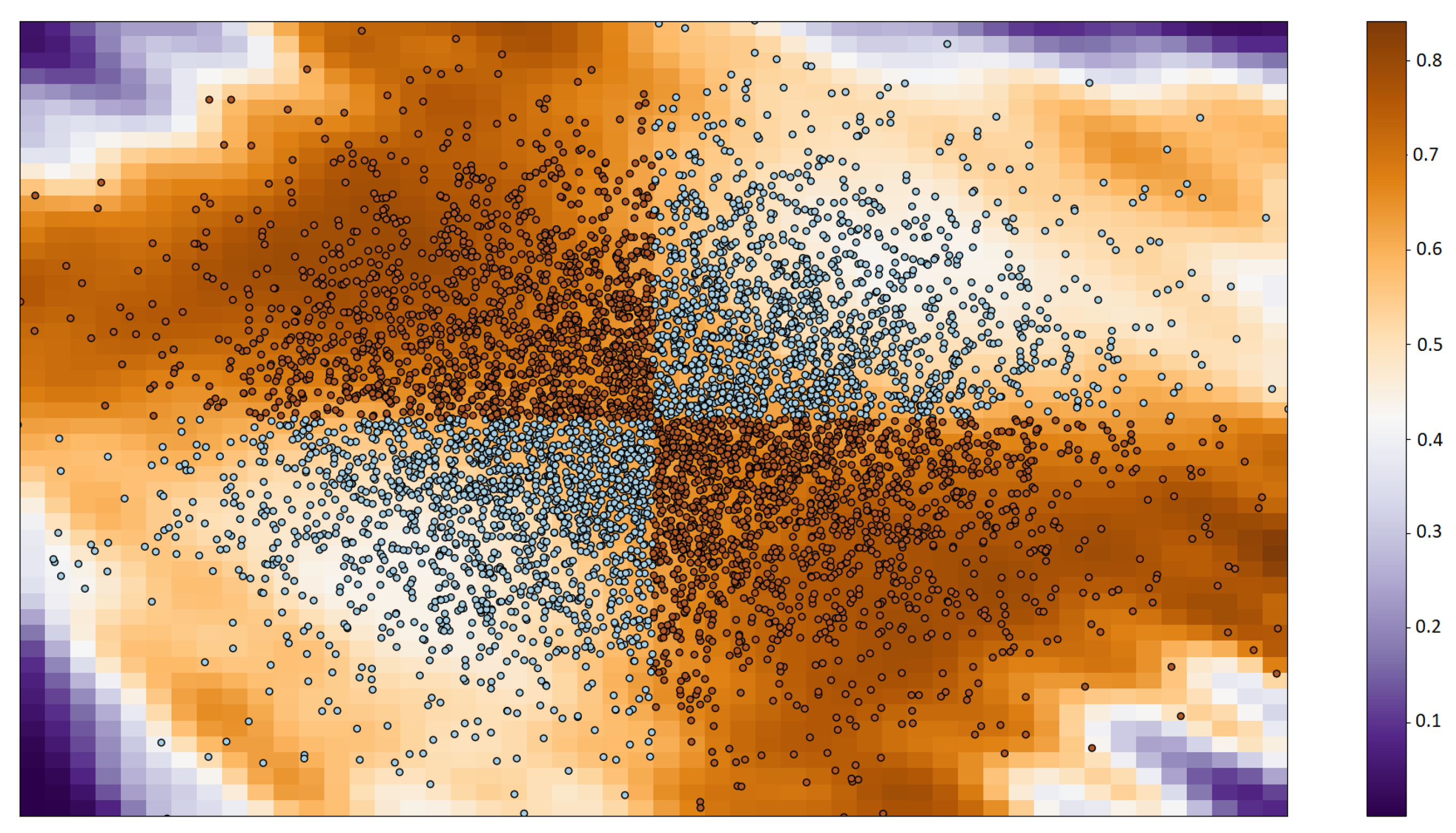
The first dataset is the XOR problem in 2D. We set the number of samples to $N=6000$. After five swaps with 300 frequencies (M), the proposal got an AUC of 0.98. The result of this experiment is shown in Figure 1.

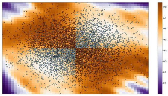
Figure 1. The XOR problem with the probability of belonging to class 1 (orange). If the probability is more than 0.5, then the sample belongs to class 1 otherwise belongs to class 2.

All the results of the GaBaSR algorithm uses 500 samples (M) and 5 swaps each one. For classification problem we use some small datasets, Breast Cancer, Credit-g, Blood Transfusion, Electricity, Egg-eye-state and Kr vs Kp. The breast cancer dataset it comes from the UCI repository [26] dataset, this dataset is the breast cancer wisconsin dataset. The Credit-g dataset comes from the UCI repository [26] and classifies people by a set of attributes as good or bad credit risk. The Electricity Dataset we downloaded from openml.org and contains data from the Australian New South Wales. Dataset egg-eye-state we downloaded from UCI, this describes if the eye is closed (1) or open (0). Kr Vs Kp dataset was downloaded from UCI, is the King Rook vs King Pawn and it’s from the King+Rook’s side to move and the classification is see if win or not win.

Table 1, Table 2 and Table 3 show the results when we try to solve the problem using perceptron, SVM and GaBaSR, respectively. From those tables, we can see that the in the problems of Kr vs. Kp and Electricity GaBaSR has "similar" AUC to SVM but it is important to notice that in blood transfusion GaBaSR performs better than the perceptron and SVM.

Table 1. Results of the Perceptron.

Dataset	N	M	Swaps	AUC
Breast Cancer [26]	569	500	5	0.96480
Credit-g [26]	1000	500	5	0.44576
Blood Transfusion [27]	748	500	5	0.37572
Electricity [28]	45,312	500	5	0.68576
Egg-eye-state [26]	14,980	500	5	0.61635
Kr vs Kp [26]	3196	500	5	0.99357

Table 2. Results SVM Classification.

Dataset	N	M	Swaps	AUC
Breast Cancer [26]	569	500	5	0.934656
Credit-g [26]	1000	500	5	0.85282
Blood Transfusion [27]	748	500	5	0
Electricity [28]	45,312	500	5	0.76076
Egg-eye-state [26]	14,980	500	5	0.692924
Kr vs Kp [26]	3196	500	5	0.96970

Table 3. Results of GaBaSR Classification.

Dataset	N	M	Swaps	AUC
Breast Cancer [26]	569	500	5	0.51348
Credit-g [26]	1000	500	5	0.5142
Blood Transfusion [27]	748	500	5	0.54063
Electricity [28]	45,312	500	5	0.74991
Egg-eye-state [26]	14,980	500	5	0.519743
Kr vs Kp [26]	3196	500	5	0.9045

In other words, if we compare Table 3 with Table 2, it is possible to observe that the results, in general, for SVM Classification are better than for GaBaSR Classification. AUC equal to 0.5 indicates that the classifier is random, so it does not fulfil its function. Comparing Table 3 with Table 2, we can conclude that SVM Classification works properly for all tested datasets except Blood Transfusion, and GaBaSR Classification works properly only for Kr vs. Kp and Electricity. Results for Blood Transfusion obtained by GaBaSR are better than for SVM but still not satisfactory. A bad result is also a result that has its value.

In general we had a good accuracy, in most of the cases we had an accuracy above 0.8. For example in the dataset for the breast cancer, we had an accuracy of 0.89, which in general is a good accuracy. In the dataset credit-g we had 0.91 of accuracy using only 500 frequencies in 5 swaps.

4.2. Regression

For the regression experiments, we use a synthetic data set in our regression attempt. For this, samples are taken from the Gaussian Mixture distribution shown in Equation (12). After that, $M=250,\mathrm{and}\mathit{\beta }\sim \mathcal{N}(0,I_{501})$ are set. In fact, the number 501 is because the extended vector is used, which takes samples from $y_i\sim \mathcal{N}({\mathit{\phi }}_{\rho }{\left(x_i\right)}^T\mathit{\beta })$, where ${\mathit{\beta }}_{\rho }$ represents the random features from $\rho$, i.e. ${\omega }_i\sim \rho \left(\omega \right),i=1,2,...,M$. Furthermore, an instance of this problem is shown in Figure 2. Also, 250 samples and vague/non-informative prior to learn the function are used, and the result is shown in Figure 3.

$$\begin{array}{cc}\hfill p\left(\omega \right)& ={\pi }_{1}p\left(\omega |0,\frac{1}{2^2}\right)+{\pi }_{2}p\left(\omega |\frac{3\pi }{4},\frac{1}{2^2}\right)+{\pi }_{3}p\left(\omega |\frac{11\pi }{8},\frac{1}{4^2}\right)\hfill \end{array}$$

(12)

$$\begin{array}{cc}\hfill \mathrm{with}& {\pi }_1={\pi }_2={\pi }_3=\frac{1}{3}\hfill \end{array}$$

(13)

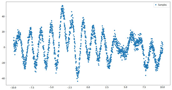
Figure 2. An instance of the samples taken from Equation (12).

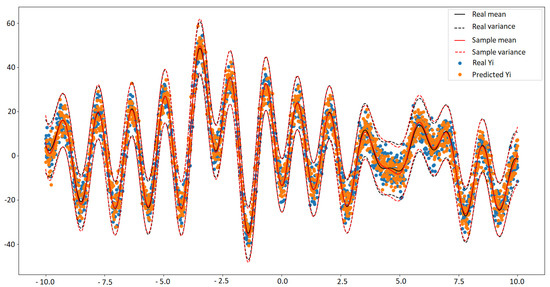
Figure 3. The real vs. predicted using GaBaSR.

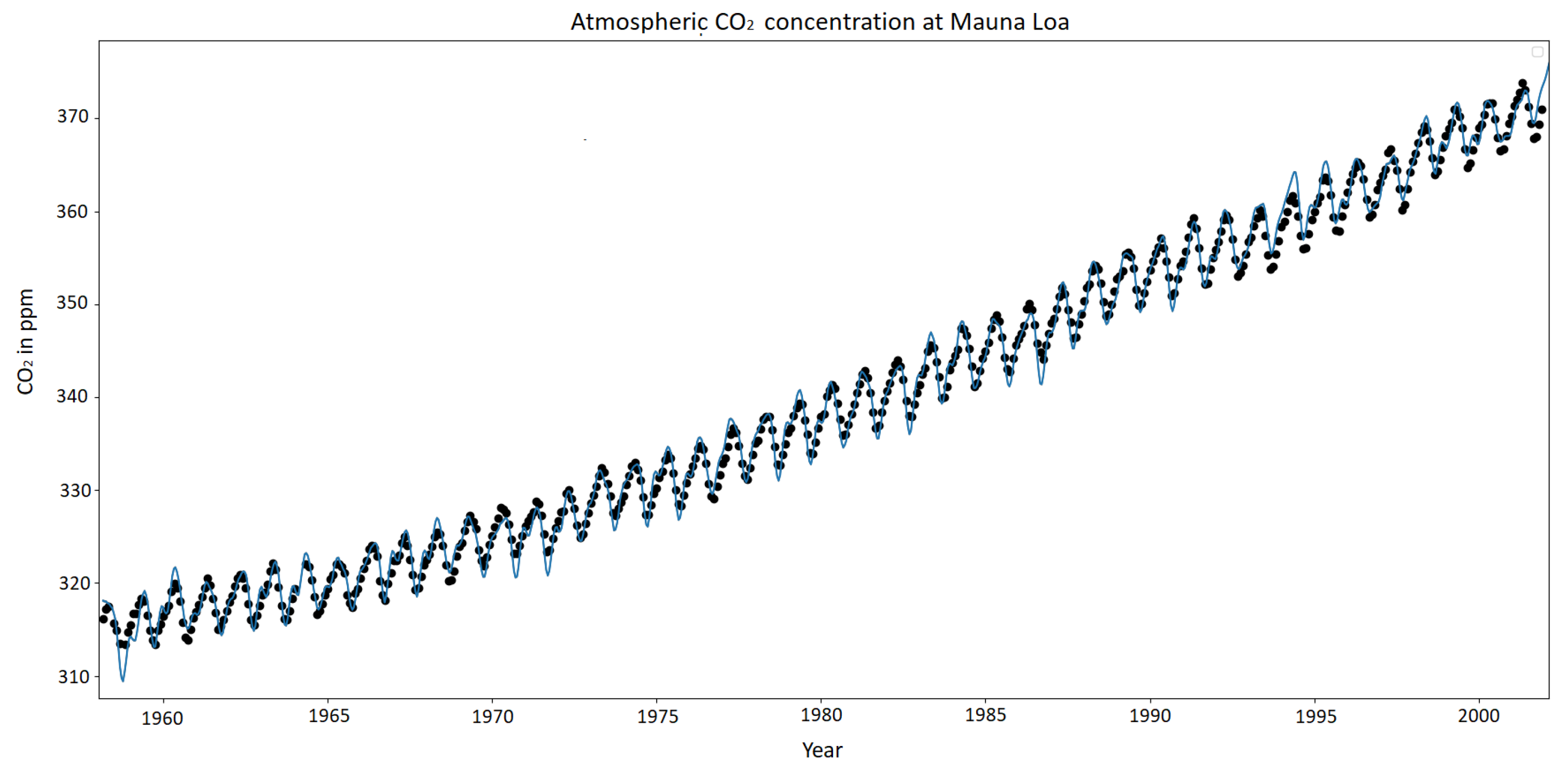
All the results of the GaBaSR algorithm uses 500 samples (M) and 5 swaps each one. For regression problems we use some small datasets, Mauna LOA CO${}_2$, California Houses, Boston house-price, and Diabetes. The Mauna LOA CO${}_2$ [29] from the global monitoring laboratory this collects the information of the monthly mean CO${}_2$, as we can see from Figure 4, this data it is stationary, has some repetitions and increments. The California Houses is a set of 20,640 rows with 8 columns. The Boston house price dataset was collected in 1978 from various suburbs in Boston. Diabetes Dataset has ten variables and the progression of the disease one year after.

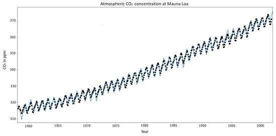
Figure 4. Mauna LOA CO${}_2$ from 1958 to 2001 and the prediction.

In this section we show three tables of results, Table 4 shows the results of our algorithm. Table 5 and Table 6 we present the results of the linear regression and the Support Vector Machine with linear kernel, respectively.

Table 4. Results GaBaSR Regression.

Dataset	M	Swaps	MSE	${\mathit{R}}^2$
Mauna LOA CO${}_2$	250	5	0.60522	0.99789
California houses	250	5	2.91313	−1.16892
Boston house-price	250	5	3.10931	0.97060
Diabetes	250	5	5,918,263.63330	−869.13210

Table 5. Results of Linear Regression.

Dataset	MSE	${\mathit{R}}^2$
Mauna LOA CO${}_2$	6.86	0.98
California houses	0.55	0.59
Boston house-price	18.92	0.78
Diabetes	3141.62	0.51

Table 6. Results Linear Regression SVM.

Dataset	MSE	${\mathit{R}}^2$
Mauna LOA CO${}_2$	758.08513	−1.60705
California houses	2.00777	−0.50784
Boston house-price	47.66904	0.43533
Diabetes	8094.08752	−0.36496

In this subsection, the experiments are performed with simple data and the result of a simple linear regression are shown. The results are shown in Table 4 and Table 5.

As it can be seen, an important result is the given by the Mauna LOA CO${}_2$ dataset. This dataset contains data from the year 1958 to 2001. Thus, for this experiment the algorithm is trained with $M=250$ and performing five swaps. After the model has been trained, to learn stationary kernels, it is possible to asses the performance of the model. For example, the achieved MSE is 0.6052 which helps at the estimation ot the CO${}_2$ outputs. For example, at the sample $2002.13$, we have prediction $376.873$ where the real measure for this value is $373.08$. The total results of Mauna LOA CO${}_2$ are shown in Figure 4 and Table 4.

We use the following datasets: (1) Mauna LOA CO${}_2$ from [29], (2) California houses from [30], (3) Boston house-price from [30] and Diabetes from [30]

5. Conclusions

Although GaBaSR’s result are promising, there are still quite a lot of work to do. For example, sampling the ${\mathit{\omega }}_j$ is quite slow, and there is a need to update the matrix $\Phi$ for only one sample. Oliva et al. [18] states that this can be done using low-rank updates. However, he does not present any procedure to perform such task, the low-rank updates are being consider for the next phase of GaBaSR. Thus, it is necessary to research how many samples M are required in order to obtain a low rank approximation.

In the experiments, it is possible to observe that GaBaSR is more accurate when performing a classification task rather than a regression task. This is an opportunity to improve the regression model. It means that the regression model needs more research to improve its performance or perhaps that a different model to learn the regression task is needed.

References

- Smola, A.J.; Schölkopf, B. Learning with Kernels; Citeseer: Princeton, NJ, USA, 1998; Volume 4. [Google Scholar]
- Soentpiet, R. Advances in Kernel Methods: Support Vector Learning; MIT Press: Cambridge, MA, USA, 1999. [Google Scholar]
- Anand, S.S.; Scotney, B.W.; Tan, M.G.; McClean, S.I.; Bell, D.A.; Hughes, J.G.; Magill, I.C. Designing a kernel for data mining. IEEE Expert 1997, 12, 65–74. [Google Scholar] [CrossRef]
- Schölkopf, B.; Smola, A.; Müller, K.R. Kernel principal component analysis. In Proceedings of the International Conference on Artificial Neural Networks, Lausanne, Switzerland, 8–10 October 1997; pp. 583–588. [Google Scholar]
- Zien, A.; Rätsch, G.; Mika, S.; Schölkopf, B.; Lengauer, T.; Müller, K.R. Engineering support vector machine kernels that recognize translation initiation sites. Bioinformatics 2000, 16, 799–807. [Google Scholar] [CrossRef] [PubMed]
- Tipping, M.E. The relevance vector machine. In Advances in Neural Information Processing Systems; MIT Press: Cambridge, MA, USA, 2000; pp. 652–658. [Google Scholar]
- Junli, C.; Licheng, J. Classification mechanism of support vector machines. In Proceedings of the WCC 2000-ICSP 5th International Conference on Signal Processing Proceedings 16th World Computer Congress, Beijing, China, 21–25 August 2000; Volume 3, pp. 1556–1559. [Google Scholar]
- Bennett, K.P.; Campbell, C. Support vector machines: Hype or hallelujah? Acm Sigkdd Explor. Newsl. 2000, 2, 1–13. [Google Scholar] [CrossRef]
- Gönen, M.; Alpaydın, E. Multiple kernel learning algorithms. J. Mach. Learn. Res. 2011, 12, 2211–2268. [Google Scholar]
- Lanckriet, G.R.; Cristianini, N.; Bartlett, P.; Ghaoui, L.E.; Jordan, M.I. Learning the Kernel Matrix with Semidefinite Programming. J. Mach. Learn. Res. 2004, 5, 27–72. [Google Scholar]
- Hoi, S.C.; Jin, R.; Lyu, M.R. Learning Nonparametric Kernel Matrices from Pairwise Constraints. In Proceedings of the 24th International Conference on Machine Learning ACM, Corvallis, OR, USA, 20–24 June 2007; pp. 361–368. [Google Scholar]
- Cvetkovic, D.M.; Doob, M.; Sachs, H. Spectra of Graphs; Academic Press: New York, NY, USA, 1980; Volume 10. [Google Scholar]
- Platt, J. Sequential Minimal Optimization: A Fast Algorithm for Training Support Vector Machines; Microsoft: Redmond, WA, USA, 1998. [Google Scholar]
- Bach, F.R.; Lanckriet, G.R.; Jordan, M.I. Multiple Kernel Learning, Conic Duality, and the SMO Algorithm. In Proceedings of the Twenty-First international Conference on Machine Learning ACM, Banff, AB, Canada, 4–8 July 2004; p. 6. [Google Scholar]
- Williams, C.K.; Rasmussen, C.E. Gaussian Processes for Machine Learning; MIT Press: Cambridge, MA, USA, 2006. [Google Scholar]
- Rahimi, A.; Recht, B. Random features for large-scale kernel machines. In Proceedings of the Advances in Neural Information Processing Systems, Vancouver, BC, Canada, 3–5 December 2007; pp. 1177–1184. [Google Scholar]
- Ghiasi-Shirazi, K.; Safabakhsh, R.; Shamsi, M. Learning translation invariant kernels for classification. J. Mach. Learn. Res. 2010, 11, 1353–1390. [Google Scholar]
- Oliva, J.B.; Dubey, A.; Wilson, A.G.; Póczos, B.; Schneider, J.; Xing, E.P. Bayesian Nonparametric Kernel-Learning. In Proceedings of the Artificial Intelligence and Statistics, Cadiz, Spain, 9–11 May 2016; pp. 1078–1086. [Google Scholar]
- Rasmussen, C. The infinite Gaussian mixture model. In Advances in Neural Information Processing Systems; MIT Press: Cambridge, MA, USA, 2000; pp. 554–560. [Google Scholar]
- Genton, M. Classes of kernels for machine learning: A statistics perspective. J. Mach. Learn. Res. 2001, 2, 299–312. [Google Scholar]
- Bochner, S. Harmonic Analysis and the Theory of Probability; California University Press: Berkeley, CA, USA, 1955. [Google Scholar]
- Silverman, R. Locally stationary random processes. IRE Trans. Inf. Theory 1957, 3, 182–187. [Google Scholar] [CrossRef]
- Hoeffding, W. Probability inequalities for sums of bounded random variables. In The Collected Works of Wassily Hoeffding; Springer: Berlin, Germany, 1994; pp. 409–426. [Google Scholar]
- Gelman, A.; Carlin, J.B.; Stern, H.S.; Dunson, D.B.; Vehtari, A.; Rubin, D.B. Bayesian Data Analysis; Chapman and Hall/CRC: Boca Raton, FL, USA, 2013. [Google Scholar]
- Geman, S.; Geman, D. Stochastic relaxation, Gibbs distributions, and the Bayesian restoration of images. IEEE Trans. Pattern Anal. Mach. Intell. 1984, 6, 721–741. [Google Scholar] [CrossRef] [PubMed]
- Dua, D.; Graff, C. UCI Machine Learning Repository. Open J. Stat. 2017, 10. [Google Scholar]
- Yeh, I.C.; Yang, K.J.; Ting, T.M. Knowledge discovery on RFM model using Bernoulli sequence. Expert Syst. Appl. 2009, 36, 5866–5871. [Google Scholar] [CrossRef]
- Gama, J. Electricity Dataset. 2004. Available online: http://www.inescporto.pt/~{}jgama/ales/ales_5.html (accessed on 6 August 2019).
- Carbon, D. Mauna LOA CO2. 2004. Available online: https://cdiac.ess-dive.lbl.gov/ftp/trends/CO2/sio-keel-flask/maunaloa_c.dat (accessed on 6 August 2019).
- Buitinck, L.; Louppe, G.; Blondel, M.; Pedregosa, F.; Mueller, A.; Grisel, O.; Niculae, V.; Prettenhofer, P.; Gramfort, A.; Grobler, J.; et al. API design for machine learning software: Experiences from the scikit-learn project. In Proceedings of the ECML PKDD Workshop: Languages for Data Mining and Machine Learning, Prague, Czech Republic, 23–27 September 2013; pp. 108–122. [Google Scholar]
Disclaimer/Publisher’s Note: The statements, opinions and data contained in all publications are solely those of the individual author(s) and contributor(s) and not of MDPI and/or the editor(s). MDPI and/or the editor(s) disclaim responsibility for any injury to people or property resulting from any ideas, methods, instructions or products referred to in the content. |
© 2023 by the authors. Licensee MDPI, Basel, Switzerland. This article is an open access article distributed under the terms and conditions of the Creative Commons Attribution (CC BY) license (https://creativecommons.org/licenses/by/4.0/).