1. Introduction
The internal communications and the refraction of information between individuals constitute numerous multi-agent systems; thus, they are important attributes of the properties that constitutes numerous natural systems. When exploring the multi-agent systems, synchronization plays an indispensable role in the power-grid networks, system biology, climatology, sociology, and technology, and especially in the consensus problem of multi-agent systems, all of which have been widely studied topic and applied in plenty of scenarios. Dynamic and self-dynamic networks, which contain linear and nonlinear parts, make the process of synchronization time-varying. These attributes make it shine in some cases, and the excessive activation and synchronization of neural networks have been found to associate with a series of dysfunctions and disorders of the brain, as well as tumor and neural diagnoses such as Parkinson’s disease, epileptic seizure, and Alzheimer’s disease. In engineering, synchronization also has important applications in smart-grid networking [
1], the industrial Internet [
2,
3], data fusion [
4,
5], and multi-agent systems [
6,
7,
8,
9]. So far, based on the computer network analysis and control theory, researchers have proposed a variety of models, algorithms, and approaches for solving the synchronization problem. The recent and specific problems are concentrated on the following directions: (1) The controllability and observability of multi-agent systems; (2) the robustness of synchronization in multi-agent systems; (3) disturbance and other restricted states; (4) the natural attributes of multi-agent systems; (5) the synchronization rate; and (6) the amount of calculation. Since we are focused on the control-oriented investigations, and simultaneously, neural networks have faced their boom era, a huge amount of computational cost pressure makes the last two directions mentioned above especially important. The mathematical analysis of synchronization is strengthened for reducing conversation [
10,
11], optimizing calculation [
12], and maximizing available resources [
13,
14] and limited application scenarios. With the deepening of research, it is becoming increasingly difficult to rely on mathematical algorithms to improve efficiency. In view of this, researchers gradually turned to other approaches.
By measuring the similarity between different data sources, and classified with multiple clusters, the pre-processing by cluster analysis can analyze various methods for different types of data, which greatly simplifies the data analysis process and is one of the most visible and explainable concepts in computer science. By applying the clustering analysis method to the large-scale complex dynamic network structure decomposition, the nodes with large correlations of properties are classified so that large-scale networks can be simplified and analyzed for a limited number of small-scale networks; thus, the network model could be simplified and the number of calculations could be reduced. The main structure of the network is also made clearer by the extraction of the main nodes. Louis M. Pecora et al. [
15] created a framework of an analysis method for network dynamics to show the connection between cluster formation and network symmetries. This finding provides the fundamental contributions to the analysis of the clustering of the dynamic network. Then, some early related applications have emerged. In [
16], based on eigenvalue decomposition, the authors proposed a centralized adaptive intermittent control approach to make cluster synchronization. By applying the adaptive approach, Tianping Chen et al. [
17] proposed sufficient conditions to guarantee global cluster synchronization for linearly coupled networks, which could be applied in neural calculation to save computations. Oriented from the pinning control strategy, the authors [
18] also found a new way to drive a general network to a selected cluster synchronization pattern. Considering an array of hybrid coupled neural networks with delay, based on Lyapunov stability theory and linear matrix inequality(LMI) method, Jinde Cao and Lulu Li [
19] proposed several sufficient conditions for cluster synchronization. It should be pointed out that compared with existing work, the coupling configuration matrix and inner coupling matrix have greater applicability. Additionally, relative works could also be seen in [
20,
21,
22,
23,
24,
25]. It is worth pointing out that there is some good work being done in some emerging and intersecting areas, such as AI-driven packet forwarding [
26] and the services of the customized industrial Internet of things [
27].
Considering that the algorithms mentioned above have made great progress in mathematics and application, the algorithms may be more complex, and many solutions are only suitable for some specific scenarios, which has led to the development of a wide range of applications and better operability. Therefore, to the author’s knowledge, there are few works on the implementation of the physical level of simplification that at the same time give the corresponding mathematical proof; this low-cost and widely used approach is also an applied method used to solve problems. In this paper, with the study of traversing binary tree theory, and the technology of cluster analysis, we proposed a network-partitioning method for pinning dynamic networks. In particular, a relative theory is proposed to guarantee all traversed nodes asymptotically synchronize to the pinning node. We have standardized this method and given one kind of specific implementation step; therefore, the main structure of the network is also highlighted. Additionally, the requirement of the application is only related to the structure of the natural structural properties of the networks and can be freely adjusted according to the actual use. The method focuses on reducing the amount of calculation, which could be applied as a pre-treatment process before most of networked synchronization algorithms. Simulations with the same algorithm show the effectiveness of the method.
The other parts are organized as follows.
Section 2 shows some preliminary knowledge of our model and introduces a description of the network partitioning problem. In
Section 3, we proposed a theorem that proves that all of the layers of the nodes in the sub-networks could synchronize to the central node.
Section 4 involves numerical simulation.
2. Preliminary Knowledge
Consider an undirected graph , where represents N notes in the graph, is the adjacency matrix, and represents an undirected edge in of the ordered pair of nodes and . is a set of undirected edges and . Without orientation, the edge of node is identical to the edge , and the information from different nodes and share the same weight. Diagonal element is defined as . It is easy to surmise that , .
We consider a common CDN with
N identical nodes of the form
where we have
is an inner-coupling matrix of appropriate dimensions,
as initial instant.
are the communication instants and satisfy
is the state vector of node
i.
d is a constant of time delay. When
,
holds at the initial condition.
To satisfy the synchronization requirement, all nodes must track the central node. In this paper, node 1 is always chosen as the central node.
Let
Therefore, we could rewrite Equation (
1) as follows:
Let
then the synchronization process could be described as
. To achieve the tracking goal, following assumption and lemma would be used.
Assumption 1 ([
28]).
A diagonal matrix exists, and then the nonlinear part of the node system satisfies the following condition: Lemma 1 ([
28]).
The following equation holds if matrix satisfies the same sum for each row.where Equation (
3) could be represented as
where
.
In practical neural networks, usually N would be a huge number; therefore, there would be a tremendous amount of . The computation burden would be enormous, although mathematical work could alleviate the problem, but the ceiling may have been encountered. Therefore, some structural approaches may be applied that may be more effective than extensive algorithms.
In our model, the structure of network is known and the central node is confirmed. For a certain single node in the networks, it is obvious that the connected edge with greater weight plays a more influential role than the smaller one. Therefore, by evaluating the influence of different connection weights of individual nodes without breaking the integrity of network structure, we could establish a rule that focuses on prior connections. The weighted edges with a strong influence could be selected and retained, and the edges with smaller weights that have trivial influence on the global synchronization target could be ignored. The structure will further save on computing resources. Based on that, the CDN with a tremendous number of nodes and connections could be partitioned by a finite number of sub-networks.
Remark 1. In the undirected graph, unlike the directed graph, usually there are no necessary pinning control networks. Therefore, throughout our paper, the central node is free to choose, and the setting of node 1 is just for convenience.
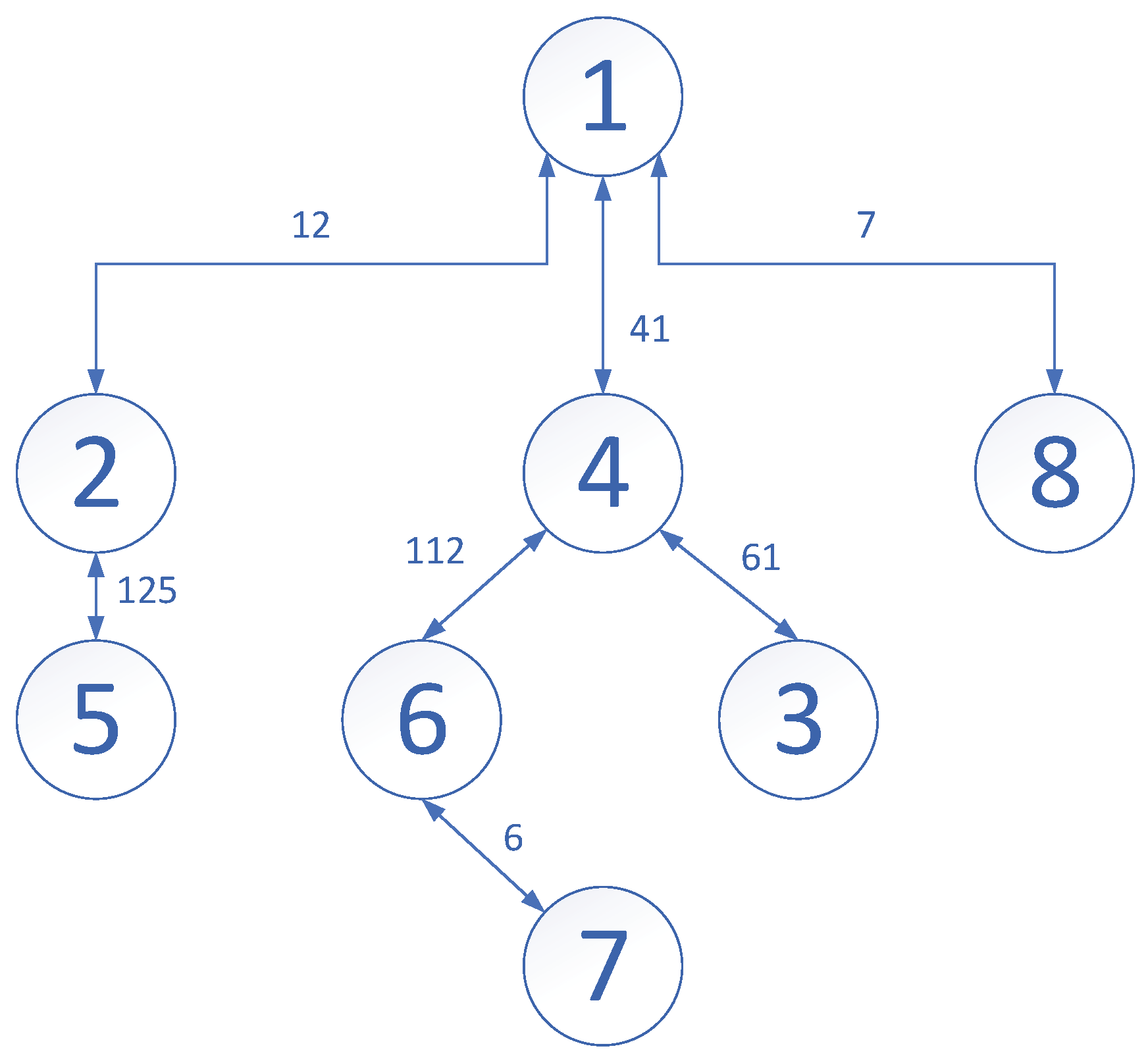
A simple example of CDN with 8 nodes is offered in
Figure 1.
The weight allocation matrix is
In
Figure 1, we can observe information transfers between node 1 and node 2, 3 and 8. Node 3 exchanges information with node 1 and 4 at the same time. For node 3, the coupling weight with node 4 is much bigger than with node 1, such that the impact from node 4 is even greater than node 1 to 3. Therefore, without affecting the complete transmission of topology, we could try to ignore the connection between node 1 and 3, to avoid useless calculations. By neglecting some trivial connections, we can realize the partitioning of the network to a finite number of sub-networks layer after layer, such that the computation burden could be relieved and the effectiveness could be boosted.
In
Figure 1, nodes 7 and 8 are the isolated nodes that only have one edge connecting to other nodes. Since node 1 is the central note, node 8 could be considered as a sub-network. As mentioned above, the connection weight between node 1 and node 3 is small. It does not affect the traversal of the whole network. Therefore, we could separate nodes 3, 4, 6, and 7 as another sub-network. Additionally, nodes 2 and 5 constitute the rest of the sub-network.
Consequently, the network of
Figure 1 could be transferred into the following
Figure 2, where the example with the form of system (
7) could be rewritten as 3 parts:
The algorithm in [
13] is applied here as reference. The total computation of scalar decision variables is
, where
,
in the example. Therefore, without partitioning the CDN, in Example 1, the number is
, while after partitioning the CDN, the number is
, which is much less than the method without partitioning the CDN.
Moreover, the advantages of partitioning will become more obvious as N increases.
Systematic process algorithms can be derived from the previous example.
3. Synchronization of Complex Dynamic Networks
Before beginning our systematic process, the integrity of information transmission should be ensured.
Throughout this paper, the synchronization algorithm is based on the following Lemma [
14].
Lemma 2. For a given scalar h, matrices , , X, , exist, and a diagonal matrix ; under Assumption 1, we havewhereThen, CDN (2) is globally exponentially synchronized. The proof process would be omitted here due to the limited space. The reader can see the whole proof process from the reference [
14].
We partition the network into finite chains, of which no cycle is included in the sub-networks. Then, the process of CDN synchronization could be reduced to the finite chains and the central note.With Lemma 2, the following theorem is proposed.
Theorem 1. Consider a class of multi-agent systems with a known structural connection weight. Partition the CDN into multi-layers of sub-networks with according sub-central nodes and stay full-connected. Assuming that each layer of the sub-network asymptotically synchronizes to the corresponding sub-central node; then, the whole CDN achieves asymptotical synchronization.
Proof. Partition the CDN with layers. Assuming that there would be sub-networks in the ith layer, therefore there would be sub-central nodes in the ith layer. denotes the jth single sub-central node. By using the prior definition, the first sub-central node is named by the 1st node, such that all nodes in the CDN could be described as . With that, we have that is the central node for all of the multi-agent systems. The sub-central node represents the jth sub-central node in the ith layer.
is the initial time. The aim is to prove that if , for any exists, and . Then, the = 0 also set up.
The proof could be achieved by the iterative method. Firstly, with the last layer, sub-networks (
th layer) asymptotically synchronize to the sub-central node
; then, the corresponding Lyapunov functional could exist and be represented as
, and we have
for all
.
Then, for the one up layer, a similar Lyapunov functional could be established with to prove that for the layer, the sub-network could achieve asymptotic synchronization.
We combine the
and
to be a new Lyapunov functional
, such that
By iterating this method over the entire network, the Lyapunov functionals could always exist
and
Such that there exist
to satisfy
□
Remark 2. In the proof, in Theorem 1, no concrete Lyapunov functional is needed to complete the proof; hence, it can be ignored.
Remark 3. Note that in the definition of , could be the same node because nodes in the th layer could the sub-central node in the th layer. The representation method does not affect the proof process.
One of the available partitioning network method is proposed with following steps:
Step 1: Lists all of the notes connected to the central node.
Step 2: Find nodes with only one connection and list them out; name these nodes “initial points”.
Step 3: Start the chain with the initial nodes. Find the node connected to the initial points, then continue the chain with the connected node to find the next step. The strategy is to connect the greater coupling weight. If the initial node only communicates with the central note, stop the search and mark the connection node as a sub-network.
Step 4: If the two chains meet at one node (not the central node), then two chains could be combined to be one chain and continue the path.
Step 5: When all of the chains are connected to the central node, mark all the chains and continue dealing with the rest of the nodes.
Step 6: Start the path from each node of the marked chain to build the sub-chain; like Step 1, the sub-central node could be set here if needed. Use the greater coupling weight strategy to connect all the other nodes.
Step 7: If two sub-chains connect to one node, the connection with stronger coupling weight could be kept as one node of the subchain. The weaker coupling weight connected node ignores this connection and searches for the second great coupling weight node.
Step 8: Repeat Step 6 until all nodes are traversed.
Step 9: After traversing all nodes in the network, the search could stop and the sub-networks could be built.
The algorithm is only a simple solution; it is not optimal. Strategies such as dynamical programming, prim’s algorithm, and others could be adopted here. Additionally, event-triggered samplers could be applied to offer a threshold. The effect of reducing the computation amount is more obvious when strategies consider more layers and a shorter chain; meanwhile, the efficiency of synchronization will be reduced by more layers. Moreover, coupling weight should also be taken into account because that will appreciably impact the synchronization rate. Therefore, the balance should be taken into account of equity simultaneously.
Remark 4. After the network-partitioning process, assuming that the new net has and by re-arranging the weight allocation matrix, the following form would be shown:where are the matrix block, and is the folded portion of the ith matrix block and is a symmetric matrix. With the re-arranged weight-allocation form, the connection between different nodes could be clarified. In our results, all of the sub-networks could be grouped into finite sub-networks that are only connected to the central node. Proofs could be offered to show where the calculation savings are coming from. This is not merely an oversight of some unnecessary coupling weights.
Before the Proof, the following assumption should be offered to make the network-partitioning process clearer.
Assumption 2. Each node in the complex networks only has one route connecting to the central node after the process of network partitioning.
Corollary 1. Considering the fully connected complex dynamic network, with the projection of network partitioning, under the condition of Assumption 1, the number of decision variables could be reduced such that the calculation could be saved.
Proof. No matter what synchronization criterion we choose, the number of decision variables will always have following form:
where
is an integer coefficient greater than or equal to zero; also,
n for the dimension of node is considered in the
.
M is the max order.
N is the number of nodes. For all of the partitioned network, the first layer only has the central node and is represented as
. In the
layer, the nodes are
, which are all sub-central nodes.
Let us start from the partitioned networks with layer 2, which means that all of the nodes are connected to the central node; therefore, we have
. Additionally, the number of decision variables could be
which is the same as the unpartitioned networks (
19). Let us extend the situation into the
layer; for the
ith layer, the
sub-central node has
sub-networks, and there are
nodes in each sub-network accordingly.
m is the serial number from
. Therefore, in the
layer, the number of decision variables we need to calculate is
where
is implemented here.
Furthermore, in each layer, the above proposition could be achieved. As the number of layers increases, the number of decision variables we need to deal with decreases at an accelerating rate.
For the central node,
represents sub-networks connected to the central node (even if only one point is included) from
to
. Additionally, the number of decision variables we have after partitioning the network is as follows:
Such that the proof is complete. □

