Ultra-High-Cycle Fatigue Life Prediction of Metallic Materials Based on Machine Learning

Abstract

The fatigue life evaluation of metallic materials plays an important role in ensuring the safety and long service life of metal structures. To further improve the accuracy and efficiency of the ultra-high-cycle fatigue life prediction of metallic materials, a new prediction method using machine learning was proposed. The training database contained the ultra-high-cycle fatigue life of different metallic materials obtained from fatigue tests, and two fatigue life prediction models were constructed based on the gradient boosting (GB) and random forest (RF) algorithms. The mean square error and the coefficient of determination were applied to evaluate the performance of the two models, and their advantages and application scenarios were also discussed. The ultra-high-cycle fatigue life of GCr15 bearing steel was predicted by the constructed models. It was found that only one datapoint of the GB model exceeded the triple error band, and the RF model had higher stability. The network model coefficient of determination and mean square error for the GB and RF models were 0.78, 0.79 and 0.69, 3.79, respectively. Both models could predict the ultra-high-cycle fatigue life of metallic materials quickly and effectively.

1. Introduction

Metal structures are generally subjected to cyclic loading during their service periods; thus, fatigue mechanisms trigger the nucleation of microcracks, crack expansion, and eventually, the complete failure of structures [1]. Due to the demand for environmental protection, metal structures should serve longer than ever, indicating that their fatigue life should exceed 10⁷ cycles (ultra-high-cycle fatigue life regime) [2]. Fatigue tests are most commonly used to predict the ultra-high-cycle fatigue life of metallic materials; however, fatigue tests are costly and time-consuming. Extensive research has been carried out to predict the ultra-high-cycle fatigue life of metallic materials more quickly and accurately [3,4,5]. Research on the fatigue life prediction of metallic materials can be divided into two main directions: physical models and data-driven models [6].

Physical models perform fatigue failure analysis and life prediction based on surface integrity factors, such as residual stress, surface roughness, internal defects, and grain size. Gao et al. [7] improved the Coffin-Mansaringeon model to increase fatigue life prediction accuracy. Li et al. [8] developed a fatigue life prediction model for surface carburized steel based on the definition of microstructures and the critical surface theory. Guo et al. [9] proposed a fatigue life prediction model using the concept of energy dissipation threshold as a failure criterion within the framework of thermodynamics. Newman Jr et al. [10] adopted the small crack theory to predict the fatigue life of two aluminum alloys and one steel alloy under different load histories. Most physical life prediction models have been developed based on fatigue damage theories, such as linear damage rules, nonlinear damage curves, two-stage linearization approach, crack growth concept, continuum damage mechanics, and energy-based theories [11]. Physical models can predict the fatigue life of metal parts to a certain extent; however, due to the disadvantages of the imperfect fatigue damage accumulation theory and the requirement of numerous model parameters, they cannot be easily used in practical engineering applications.

Data-driven models determine the relationship between the input and output of a given phenomenon based on available data [12]. With the development of artificial intelligence, machine learning (ML) has created more opportunities for data-driven models. Zhan et al. [13] proposed a damage mechanics-based machine learning framework for the data-driven fatigue life prediction of titanium alloys. Dang et al. [14] used a support vector regression (SVR) algorithm to develop a fatigue life prediction model by post mortem fractography analysis. Wang et al. [15] used a BP neural network to predict the VHCF life of centrifugal impeller blades. Zhang et al. [16] applied a neuro-fuzzy-based machine learning approach to predict the high-cycle fatigue life of laser powder bed-fused 316 L stainless steel. Pierson K. et al. [17] explored the use of ML to predict the microstructural sensitivity of three-dimensional (3D) crack surfaces in polycrystalline alloys. Raja A. et al. [18] investigated the relationship between the fatigue crack growth rate (da/dN) and the stress intensity factor range (∆K) by a machine learning model and reported that the application of machine learning to fatigue life prediction could be feasible. However, current data-driven fatigue life prediction models have the disadvantage of difficult access to input parameters and single application scenarios. For example, Dang et al. [14] used material microscopic properties as input parameters, which were difficult to be obtained and very expensive, to develop fatigue life prediction models. Thus, it is necessary to find a fatigue life prediction model with simple input parameters.

In the present study, an ultra-high-cycle fatigue life database containing ten types of metals was constructed, and subsequently fatigue life prediction models were built based on the gradient boosting (GB) and random forest (RF) algorithms. The mean square error and the neural network decision coefficient were used to evaluate the performance of the two models, and their advantages and application scenarios were also discussed. Finally, the generalization abilities of the models were evaluated by predicting the ultra-high-cycle fatigue life of GCr15-bearing steel. The models constructed in this work required simple input parameters and manifested excellent fatigue life prediction ability.

2. Database and Machine Learning Algorithms

2.1. Database

Conventional ultra-high-cycle fatigue tests are very time-consuming and take nearly four days to complete 10⁷ cycles at a frequency of 30 Hz; however, 20 kHz ultrasonic fatigue experiments consume at least 400 times less time than conventional ones [19]. Therefore, the establishment of a database based on ultrasonic fatigue experiments can reduce the test time during the model validation phase and also facilitate the replenishment of the database in the future. In this study, 84 ultrasonic fatigue experimental datapoints were collected from published works to establish a database. The database contained commonly used metals in engineering and materials formed by special methods (for example, GH4169 alloy formed by selective laser melting). It should be noted that the loading conditions for all ten materials were ultrasonic and the loading stress ratio was −1. Ultrasonic fatigue tests were conducted in a stress range of 100–900 MPa, and the fatigue life of all ten materials was achieved at 10⁷ cycles. The data sources and the test conditions are listed in

Table 1. Training database.

Materials	Machine Model	Loading Frequency	Stress Ratio	Number of Data	References
TC32 titanium alloy	USF-2000	20 kHz	−1	10	Literature [20]
X80 acicular ferrite	USE-2000	20 kHz	−1	8	Literature [21]
Ti60 titanium alloy	Self-developed	20 kHz	−1	6	Literature [22]
TC11 titanium alloy	Unknown	20 kHz	−1	10	Literature [23]
GH4169 alloy	USF-300	20 kHz	−1	8	Literature [24]
54SiCrV6 steel	USF-2000	20 kHz	−1	13	Literature [25]
ZK60 magnesium alloy	USF-2000	20 kHz	−1	9	Literature [26]
AA2198-T8 aluminum alloy	USF-2000	20 kHz	−1	8	Literature [27]
Ti-6Al-4V titanium alloy	Unknown	20 kHz	−1	7	Literature [28]
16MnR steel	Unknown	20 kHz	−1	5	Literature [29]

, and the stress distributions of the materials are shown in Figure 1. It should be noted that GCr15-bearing steel was not involved in the training of the model, but only as a final test of the model.

2.2. Machine Learning Algorithms

Artificial neural networks are inspired by brain perceptual processing. Computational algorithms are used to simulate brain neurons and allow models to learn autonomously to solve different types of problems [30].

Gradient boosting is a powerful machine-learning technique [31]. The main idea of this algorithm is to cascade the level of learners and use the errors of the previous learner for reinforcement in the current learner. The overall model error gets gradually reduced, and the improvement of model accuracy is eventually achieved. The specific implementation process is divided into four steps. Total data set S = {(x₁, y₁), (x₂, y₂), …, (x_n, y_n)}. The loss function is L (y, f (x)). The nodes of the regression tree are J. Partition the input space into j disjoint regions (R₁, R₂, …, R_j). Estimate a constant value for each region b_j. The regression tree equations are as

$$g_m(x)={\displaystyle \sum _{j=1}^j(b_{j}k)},x\subset R_j$$

(1)

$$k(x\subset R_j)=\left\{\begin{array}{l}1,x\subset R_j\\ 0,x\not\subset R_j\end{array}\right.$$

(2)

(1)

Initialize the model by

$$f_0(x)=\underset{c}{\arg \min }{\displaystyle \sum _{i=1}^{n}L(y_i,c)}$$

(3)

(2)

Calculate the residuals by

$$r_{im}=-{\left[\frac{\partial L(y_i,f_{m-1}(x_i)}{\partial f_{m-1}(x_i)}\right]}_{f(x)=f_{t-1}(x)}$$

(4)

where m and t denote number of samples and iterations.

(3)

Calculate the step size of gradient descent by

$$c_m=\arg \min {\displaystyle \sum _{i=1}^{n}L(y_i,f_{m-1}(x_i)+c{g}_m(x_i))}$$

(5)

(4)

Update model by

$$f_m(x)=f_{m-1}(x)+Lr\times c_m{g}_m(x)$$

(6)

where Lr denotes learning rate.

The random forest algorithm has gained much attention in different industries due to its efficiency and accuracy [32]. The core idea of this technique is to select the output results of several weak classifiers by voting to form a strong classifier. RF is a begging integration model, and it can be divided into three phases.

(1)

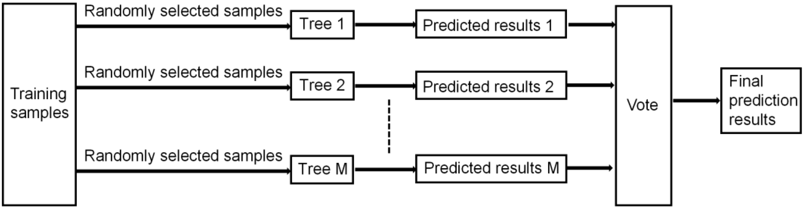
Sampling with put-back is performed on samples (one sample is selected randomly each time). The selected N number of samples is then used to train a decision tree as samples at the root node of the decision tree. N subsets of samples are obtained, denoted as N_i (i = 1, 2, …, k).

(2)

Each sample has M attributes. When each node of the decision tree needs to be split, m attributes are randomly selected from these M attributes to satisfy the following condition: m<<M. One attribute is then selected from these m attributes as the splitting attribute for that node. If the attribute selected by the next node is the attribute used in the last split of its parent node, the node reaches a leaf node and the splitting process stops. Build a regression model for each subset of samples, denoted as {f(x,o_i), i = 1, 2, …, k}, where the matrix x is the independent variable for modeling, and the set of parameters o_i is independently distributed.

(3)

After k rounds of training, a sequence of regression tree models {f₁(x), f₂(x), … f_k(x)} is obtained. The output function of the kth decision tree can be described as

$$fr(x)=\frac{1}{k}{\displaystyle \sum _{i=1}^k{f}_k(x)}$$

(7)

where f_r(x) denotes the prediction of RF for target variables.

The RF model uses parallel generation, whereas the GB model applies serial generation. The implementation processes of the GB and RF models are illustrated in Figure 2 and Figure 3, respectively.

3. Model Presentation

3.1. Determination of Input Parameters

The study of Lei He [33] on machine learning for the fatigue life prediction of steel pointed out that the static mechanical properties of the material affected its fatigue life. Xue et al. [34] found that in ultrasonic fatigue experiments, specimen size had a significant effect on ultra-high-cycle fatigue life, and fatigue strength decreased with the increase in specimen size. Hence, the modulus of elasticity (E), tensile strength (${\mathsf{\sigma }}_{\mathrm{b}}$), yield strength (${\mathsf{\sigma }}_{0.2}$), density ($\mathsf{\rho }$), elongation after fracture (A), and ultrasonic fatigue specimen geometry were selected as input parameters for the proposed models. Round specimens were used in ultrasonic fatigue tests because they are easy to be processed and have large displacement stress factors. All fatigue test specimens adopted a circular arc shape (Figure 4). In the determination of ultrasonic fatigue specimen geometry, specimen dimensions must satisfy the resonance equation [19]. The resonance equation indicates that the overall specimen size can be determined based on any three geometric dimensions. Therefore, the input parameters for ultrasonic fatigue specimen geometry were selected as R₁, R₂, and L₁. The input parameters of the ten materials are listed in

Table 2. Input parameters of the ten materials.

Materials	E (MPa)	${\mathsf{\sigma }}_{\mathbf{b}} \left(\mathbf{MPa}\right)$	${\mathsf{\sigma }}_{0.2} \left(\mathbf{MPa}\right)$	$\mathsf{\rho }$ (g/cm3)	A (%)	R1 (mm)	R2 (mm)	L1 (mm)
TC32 titanium alloy [20]	111	1380	1215	4.54	14.8	1.5	5	20
X80 acicular ferrite [21]	209	688	564	7.99	28	1.5	5	20
Ti60 titanium alloy [22]	114	1044	934	6.79	11	2	5	13
TC11 titanium alloy [23]	114	1132	971	4.48	16.5	1.5	6	15
GH4169 alloy [24]	191	1289	992	8.69	15.3	1.5	5	12
54SiCrV6 steel [25]	209	1743	1573	7.75	12	1.5	5	20
ZK60 magnesium alloy [26]	45	305	235	1.82	11	1.5	3.5	15
AA2198-T8 aluminum alloy [27]	71	597	538	2.79	9.9	1.5	5	14.3
Ti-6Al-4V titanium alloy [28]	106	1009	891	4.44	10	1.5	5	14
16MnR steel [29]	209	582	378	7.85	21	1.5	5	14

. It is important to note that numerous other variables are not described in this paper; however, they have great impacts on the fatigue life of materials. For example, surface defects can significantly affect the ultra-high-cycle fatigue life of materials. In the future, these variables will be investigated to further improve the accuracy of fatigue life prediction models.

3.2. Data Processing

The collected data were pre-processed to speed up the optimal solution and improve the accuracy of the models. Linear normalization was used for the input parameters [35].

$$X^{\prime }=\frac{X-X_{min}}{X_{max}-X_{min}}$$

(8)

where $X$ and $X^{\prime }$ denote the original data value and the normalized value, respectively, whereas $X_{max}$ and $X_{min}$ represent the maximum and minimum values of the original data, respectively.

The order of magnitude for the output parameters ranged between 10⁴ and 10⁹, and it was normalized nonlinearly [33] as

$$Y=ln\left(N_f\right)$$

(9)

where $Y$ is the true fatigue life and $N_f$ denotes the normalized fatigue life. The fatigue life values predicted by the models were obtained by inverse normalization.

3.3. Model Implementation

The numbers of nodes in the input and output layers of the models were 8 and 1, respectively. Hidden nodes were determined as

$$N^{\prime }=\sqrt{N+M}+a$$

(10)

where $N$ and $M$ denote the numbers of input and output nodes, respectively (ranged between 1 and 10), and $N^{\prime }$ is the number of hidden nodes. In the model training phase, the number of hidden nodes was varied to determine the best-fitted number. The numbers of nodes for the RF and GB models were 17 and 18, respectively.

Figure 5 illustrates the general implementation steps of machine learning. It is noticeable that the implementation process can be divided into a training phase and a testing phase. The training phase consists of the optimization of weights and biases and the tuning of hyperparameters. The testing phase is designed to evaluate the learning effect of the model and adjust the parameters based on the obtained result.

4. Model Evaluation and Comparison

The mean square error (MSE) [36] and the coefficient of determination (R²) [36] were adopted as prediction error metrics to compare the two models quantitatively.

$$MSE=\frac{{{\displaystyle \sum }}_{i=1}^n{(\widetilde{Y_i}-Y_i)}^2}{n}$$

(11)

$$R^2=1-\frac{{{\displaystyle \sum }}_{i=1}^n{(\widetilde{Y_i}-Y_i)}^2}{{{\displaystyle \sum }}_{i=1}^n{(\overline{Y_i}-Y_i)}^2}$$

(12)

where $\widetilde{Y_i}$ is the predicted life, $Y_i$ is the actual life, and $\overline{Y_i}$ denotes the average of the actual life. The smaller the $MSE$ value or the larger the $R^2$ value, the better the prediction performance. In addition, the generalization capabilities of the models were analyzed by predicting the fatigue life of GCr15 bearing steel.

4.1. Evaluation of Model Accuracy and Stability

The dataset was divided into two different proportions to investigate the impact of training dataset size on the performance of the machine learning models. The cases with 80% and 60% of the total training data were labeled as Case 80-20 (67 data for training and 17 data for testing) and Case 60-40 (50 data for training and 34 data for testing), respectively. It should be emphasized that the database was randomly disrupted before data partitioning to ensure the consistency of the two partitioning methods. To evaluate the models accurately, each model was trained and predicted ten times, and subsequently the best prediction was selected to illustrate prediction accuracy. Figure 6 compares the predicted and experimental fatigue life values for the two data division cases (the solid black lines indicate that the predicted and experimental values are equal, and the two black dashed lines are threefold error bands).

It is evident that the prediction accuracy of both models was improved greatly as the proportion of training data increased, implying that the size of training data significantly affected the accuracy of the models. The GB model predicted more accurately than the RF model. Both models had a conservative tendency for the prediction of 10⁷–10⁹ lifetimes, indicating that the predicted lifetimes were smaller than the experimental ones; however, for the prediction of lifetimes below 10⁷ cycles, the predicted values were larger, and these two prediction tendencies were more obvious in the RF model. The GB model took three times longer consumption time than the RF model, and it happened because the RF model used parallel generation, whereas the GB model adopted serial generation. In addition, the RF model predicted less volatility in the results. For example, during the fatigue life prediction of TC11 under 570 MPa, the variance of the ten predicted fatigue life values for the RF and GB models was 0.46 and 3.86, respectively. The RF model emphasizes stable prediction to ensure control, whereas the GB model is more suitable for scenarios where prediction accuracy is the primary goal.

4.2. Evaluation of Model Generalization Ability

Ultrasonic fatigue tests were performed on GCr15-bearing steel to obtain its fatigue life. The experimentally obtained fatigue lifetimes were then compared with the predicted values to evaluate the generalization abilities of the models. From Figure 1, the S–N curves of GCr15-bearing steel contained five stress levels and its fatigue life was distributed between 10⁴ and 10⁸ with a total of 12 data points.

All data in the database were used for model training, and fatigue life prediction was then performed for GCr15 bearing steel. It was found that the predicted life fluctuated greatly. For example, in some cases, the values of R² were close to zero, indicating that the models had a certain degree of degradation in their fatigue life prediction ability for new materials. It is already pointed out that training dataset size could significantly affect model accuracy. Gan et al. [37], in their study on fatigue life prediction under average stress using the RF algorithm and limited learning, also found that prediction ability was significantly improved when local or global similarities were involved between the new material and the material in the training. Therefore, three new experimental datasets of GCr15-bearing steel were added to the training database to expand the training dataset and introduce local similarities. The input parameters of GCr15-bearing steel are listed in

Table 3. Input parameters of GCr15-bearing steel.

Variable	Value	Variable	Value
E (GPa)	210	A (%)	24
${\mathsf{\sigma }}_{\mathrm{b}}$ (MPa)	857	R1 (mm)	1.5
${\mathsf{\sigma }}_{0.2}$ (MPa)	756	R2 (mm)	4
$\mathsf{\rho }$ (g/cm3)	7.81	L1 (mm)	15

. Ten fatigue life outputs were performed for each stress level, and the output life closest to the experimental data was selected as the prediction result. The fatigue life prediction results of the two models are compared with the experimental values in Figure 7.

With the addition of the three new experimental datasets of GCr15-bearing steel to the training database, the value of R² did not appear close to zero, improving the prediction capability of the models. The GB model had only one data point outside the triple error bands, whereas the RF model had only three data points within the triple error bands. The prediction accuracy of the GB model was better than that of the RF model. However, the RF model had better prediction stability than the GB model. Figure 8 compares the fatigue life prediction abilities of the two models for GCr15 bearing steel under 450 MPa for ten times, and it is noticeable that the GB model had two flaw points, whereas the prediction results of the RF model did not have large deviations. Figure 7 reveals that both models had a conservative tendency in making predictions for lifetimes above 10⁷ cycles. With the introduction of local similarities, both models could make good predictions for the fatigue life of new materials and maintain their respective advantages.

Table 4. Relative errors of the predicted and experimental data for GCr15 bearing steel.

Stress Amplitude (MPa)	490	490	480	480	470	470	470	470	460	460	460	450
Relative error of the GB model (%)	4.92	3.55	1.4	5.24	10.56	9.31	5.42	1.96	0.76	4.17	14.75	0.69
Relative error of the RF model (%)	16.84	15.31	23.78	18.95	18.15	16.81	12.65	8.96	1.93	3.06	13.76	0.93

presents the relative errors of the predicted and experimental values. The relative error of RF model is larger than GB.

Therefore, it can be inferred that the prediction ability of the two models for new materials was largely limited by the training database. With the introduction of local similarities, the prediction ability of the models was significantly improved. It is certain that with the progress of ultrasonic fatigue research, more materials will be added to the database and similarities between materials to be predicted and training materials will be further improved.

4.3. Comparison with Other Models

The fatigue life prediction abilities of the GB and RF models were compared with those of other models. The prediction results of the ANN algorithm for AM stainless steel 316L [36] and five models considering the effect of the mean stress for 2.2Ni–1Cr–0.5Mo–0.1 V steel [37] are presented in Figure 9 and Figure 10. The prediction results of the GBR algorithm for aluminum alloy [38] are shown in Figure 11. In terms of R² and MSE, the prediction accuracy of the GB model was higher than those of the MORROW, SWT, and FS models. The models of Figure 10 used twelve input parameters, whereas the models used in this work used eight input parameters. Therefore, the models proposed in this analysis ensured better prediction accuracy with lower input parameters. In addition, the model developed in this study has wider applicability. The ANN model developed by Zhan et al. applies to 316L, while the GBR model developed by Lian et al. applies to aluminum alloys.

5. Conclusions

To predict the ultra-high-cycle fatigue life of metallic materials, two ultra-high-cycle fatigue life prediction models were developed based on the GB and RF algorithms. The fatigue life of materials was obtained by inputting the partial mechanical properties of the materials and the geometry of ultrasonic fatigue specimens, largely reducing the cost of obtaining the fatigue life of metallic materials. The main observations of this work are presented below.

(1)

The training data size significantly affected the accuracy of the models. As the proportion of training data increased, the prediction ability of both GB and RF models was significantly improved.

(2)

The GB and RF models manifested different characteristics in predicting the fatigue life of metallic materials. The GB model had higher prediction accuracy than the RF model, whereas the RF model had better stability. In practical applications, they could be used alone or in combination to suit different scenarios.

(3)

Local similarities were introduced to the models. The fatigue life prediction ability of the GB and RF models for new materials was significantly improved by adding data of new materials to the training database.

References

1. Shanyavsky, A.A. Scales of metal fatigue cracking. Phys. Mesomech. 2015, 18, 163–173. [Google Scholar] [CrossRef]
2. Wang, Q.; Khan, M.K.; Bathias, C. Current understanding of ultra-high cycle fatigue. Theor. Appl. Mech. Lett. 2012, 2, 031002. [Google Scholar] [CrossRef] [Green Version]
3. Jang, J.; Khonsari, M.M. On the prediction of fatigue life subjected to variable loading sequence. Fatigue Fract. Eng. Mater. Struct. 2021, 44, 2962–2974. [Google Scholar] [CrossRef]
4. Miner, M.A. Cumulative Damage in Fatigue. J. Appl. Mech. 1945, 12, A159–A164. [Google Scholar] [CrossRef]
5. Forman, R.G.; Kearney, V.E.; Engle, R.M. Numerical analysis of crack propagation in cyclic-loaded structures. J. Basic Eng. 1967, 89, 459–463. [Google Scholar] [CrossRef]
6. Mosallam, A.; Medjaher, K.; Zerhouni, N. Data-driven prognostic method based on Bayesian approaches for direct remaining useful life prediction. J. Intell. Manuf. 2016, 27, 1037–1048. [Google Scholar] [CrossRef] [Green Version]
7. Gao, L.; Sun, C.; Zhuang, M.L.; Hou, M. Fatigue life prediction of HTRB630E steel bars based on modified coffin-manson model under pre-strain. In Structures; Elsevier: Amsterdam, The Netherlands, 2022; Volume 38, pp. 28–39. [Google Scholar]
8. Li, C.; Zhang, Y.; Cai, L.; Hu, T.; Wang, P.; Li, X.; Sun, R.; Li, W. A fatigue life prediction approach to interior cracking induced high cycle and very high cycle fatigue for surface-carburized steels. Fatigue Fract. Eng. Mater. Struct. 2022, 45, 865–881. [Google Scholar] [CrossRef]
9. Guo, Q.; Zaïri, F.; Guo, X. An intrinsic dissipation model for high-cycle fatigue life prediction. Int. J. Mech. Sci. 2018, 140, 163–171. [Google Scholar] [CrossRef]
10. Newman, J.C., Jr.; Phillips, E.P.; Swain, M.H. Fatigue-life prediction methodology using small-crack theory. Int. J. Fatigue 1999, 21, 109–119. [Google Scholar] [CrossRef] [Green Version]
11. Fatemi, A.; Yang, L. Cumulative fatigue damage and life prediction theories: A survey of the state of the art for homogeneous materials. Int. J. Fatigue 1998, 20, 9–34. [Google Scholar] [CrossRef]
12. Spear, A.D.; Kalidindi, S.R.; Meredig, B.; Kontsos, A.; Le, J.B. Data-driven materials investigations: The next frontier in understanding and predicting fatigue behavior. JOM 2018, 70, 1143–1146. [Google Scholar] [CrossRef] [Green Version]
13. Zhan, Z.; Hu, W.; Meng, Q. Data-driven fatigue life prediction in additive manufactured titanium alloy: A damage mechanics based machine learning framework. Eng. Fract. Mech. 2021, 252, 107850. [Google Scholar] [CrossRef]
14. Dang, L.; He, X.; Tang, D.; Li, Y.; Wang, T. A fatigue life prediction approach for laser-directed energy deposition titanium alloys by using support vector regression based on pore-induced failures. Int. J. Fatigue 2022, 159, 106748. [Google Scholar] [CrossRef]
15. Jinlong, W.; Wenjie, P.; Yongjie, B.; Yuxing, Y.; Chen, C. VHCF evaluation with BP neural network for centrifugal impeller material affected by internal inclusion and GBF region. Eng. Fail. Anal. 2022, 136, 106193. [Google Scholar] [CrossRef]
16. Zhang, M.; Sun, C.N.; Zhang, X.; Goh, P.C.; Wei, J.; Hardacre, D.; Li, H. High cycle fatigue life prediction of laser additive manufactured stainless steel: A machine learning approach. Int. J. Fatigue 2019, 128, 105194. [Google Scholar] [CrossRef]
17. Pierson, K.; Rahman, A.; Spear, A.D. Predicting microstructure-sensitive fatigue-crack path in 3D using a machine learning framework. JOM 2019, 71, 2680–2694. [Google Scholar] [CrossRef] [Green Version]
18. Raja, A.; Chukka, S.T.; Jayaganthan, R. Prediction of fatigue crack growth behaviour in ultrafine grained al 2014 alloy using machine learning. Metals 2020, 10, 1349. [Google Scholar] [CrossRef]
19. Bathias, C. Piezoelectric fatigue testing machines and devices. Int. J. Fatigue 2006, 28, 1438–1445. [Google Scholar] [CrossRef]
20. Wang, Z.; Wang, X.; Meng, Y.; Zheng, Y.; Zhao, Z. Study on ultra-high cycle fatigue performance of TC32 titanium alloy. Heat Treat. Met. 2019, 44, 595–598. [Google Scholar]
21. Zhang, J. Very high cycle fatigue behavior of X80 acicular ferrite line pipe. Trans. Mater. Heat Treat. 2020, 41, 144–150. [Google Scholar]
22. He, R.; Peng, H.; Liu, F.; Khan, M.K.; Chen, Y.; He, C. Crack Initiation Mechanism and Life Prediction of Ti60 Titanium Alloy Considering Stress Ratios Effect in Very High Cycle Fatigue Regime. Materials 2022, 15, 2800. [Google Scholar] [CrossRef] [PubMed]
23. Gao, T.; Xue, H.; Sun, Z.; Retraint, D. Investigation of crack initiation mechanism of a precipitation hardened TC11 titanium alloy under very high cycle fatigue loading. Mater. Sci. Eng. A 2020, 776, 138989. [Google Scholar] [CrossRef]
24. Song, Z.X.; Wang, D.; Wu, Z.; Sun, K.; Wu, H.; Liu, X. Ultrahigh cycle fatigue performance of GH4169 alloy by selective laser melting. Mater. Mech. Eng. 2020, 44, 72–77. [Google Scholar]
25. Zhang, J.M.; Yang, Z.G.; Li, S.X.; Li, G.Y.; Hui, W.J.; Weng, Y.Q. Ultra high cycle fatigue behavior of automotive high strength spring steels 54SiCrV6 and 54SiCr6. Acta Metall. Sin. 2006, 42, 259–264. [Google Scholar]
26. Chen, Y.; He, C.; Liu, F.; Wang, C.; Xie, Q.; Wang, Q.; Liu, Y. Effect of microstructure inhomogeneity and crack initiation environment on the very high cycle fatigue behavior of a magnesium alloy. Int. J. Fatigue 2020, 131, 105376. [Google Scholar] [CrossRef]
27. Xu, L.; Wang, Q.; Zhou, M. Micro-crack initiation and propagation in a high strength aluminum alloy during very high cycle fatigue. Mater. Sci. Eng. A 2018, 715, 404–413. [Google Scholar] [CrossRef]
28. Cao, X.; Wang, Q.; Chen, G.; Dou, Q.; Song, Z.; Wang, H. Influence of subjection to physiological saline solution on Ultra-high cycle fatigue properties of TC4. J. Southwest Univ. Sci. Technol. 2007, 22, 5–8. [Google Scholar]
29. Chen, S.; Liu, R.; Ouyang, Q.; Wang, Q.; Dong, S. Study on the Ultrasonic fatigue test of 16MnR. J. Southwest Univ. Sci. Technol. 2009, 24, 29–32. [Google Scholar]
30. Krogh, A. What are artificial neural networks? Nat. Biotechnol. 2008, 26, 195–197. [Google Scholar] [CrossRef]
31. Natekin, A.; Knoll, A. Gradient boosting machines, a tutorial. Front. Neurorobotics 2013, 7, 21. [Google Scholar] [CrossRef] [Green Version]
32. Iverson, L.R.; Prasad, A.M.; Matthews, S.N.; Peter, M. Estimating potential habitat for 134 eastern US tree species under six climate scenarios. For. Ecol. Manag. 2008, 254, 390–406. [Google Scholar] [CrossRef]
33. He, L.; Wang, Z.L.; Akebono, H.; Sugeta, A. Machine learning-based predictions of fatigue life and fatigue limit for steels. J. Mater. Sci. Technol. 2021, 90, 9–19. [Google Scholar] [CrossRef]
34. Xue, H.; Sun, Z.; Zhang, X.; Gao, T.; Li, Z. Very high cycle fatigue of a cast aluminum alloy: Size effect and crack initiation. J. Mater. Eng. Perform. 2018, 27, 5406–5416. [Google Scholar] [CrossRef]
35. Abd Elaziz, M.; Abo Zaid, E.O.; Al-qaness, M.A.A.; Ibrahim, R.A. Automatic Superpixel-Based Clustering for Color Image Segmentation Using q-Generalized Pareto Distribution under Linear Normalization and Hunger Games Search. Mathematics 2021, 9, 2383. [Google Scholar] [CrossRef]
36. Zhan, Z.; Li, H. Machine learning based fatigue life prediction with effects of additive manufacturing process parameters for printed SS 316L. Int. J. Fatigue 2021, 142, 105941. [Google Scholar] [CrossRef]
37. Gan, L.; Wu, H.; Zhong, Z. Fatigue life prediction considering mean stress effect based on random forests and kernel extreme learning machine. Int. J. Fatigue 2022, 158, 106761. [Google Scholar] [CrossRef]
38. Lian, Z.H.; Li, M.J.; L., W.C. Fatigue life prediction of aluminum alloy via knowledge-based machine learning. Int. J. Fatigue 2022, 157, 106716. [Google Scholar] [CrossRef]
Figure 1. S–N curves of the eleven alloys used in the dataset.
Applsci 13 02524 g001
Figure 2. Illustration of the GB architecture.
Applsci 13 02524 g002
Figure 3. Illustration of the RF architecture.
Applsci 13 02524 g003
Figure 4. Specimen geometry for ultrasonic fatigue tests.
Applsci 13 02524 g004
Figure 5. Machine learning process.
Applsci 13 02524 g005
Figure 6. Predicted fatigue life values for Case 60-40 ((A) GB and (B) RF) and Case 80-20 ((C) GB and (D) RF).
Applsci 13 02524 g006
Figure 7. Predicted fatigue life values for GCr15-bearing steel based on the GB and RF models.
Applsci 13 02524 g007
Figure 8. Predicted fatigue life values for GCr15-bearing steel at 450 MPa based on the GB and RF models.
Applsci 13 02524 g008
Figure 9. Comparison of the predicted and experimental fatigue life values for AM stainless steel 316L based on ANN [36].
Applsci 13 02524 g009
Figure 10. Comparison of the predicted and experimental fatigue life values for 2.2Ni–1Cr–0.5Mo–0.1 V steel [37].
Applsci 13 02524 g010
Figure 11. Comparison of the predicted and experimental fatigue life values for aluminum alloy based on GBR [38].
Applsci 13 02524 g011