Article

Human Pose Estimation Using MediaPipe Pose and Optimization Method Based on a Humanoid Model

Department of Electronics Engineering, Seunghak Campus, Dong-A University, Busan 49315, Republic of Korea
*
Author to whom correspondence should be addressed.
Appl. Sci. 2023, 13(4), 2700; https://doi.org/10.3390/app13042700
Submission received: 4 January 2023 / Revised: 10 February 2023 / Accepted: 15 February 2023 / Published: 20 February 2023
(This article belongs to the Section Computing and Artificial Intelligence)

Abstract

:
Seniors who live alone at home are at risk of falling and injuring themselves and, thus, may need a mobile robot that monitors and recognizes their poses automatically. Even though deep learning methods are actively evolving in this area, they have limitations in estimating poses that are absent or rare in training datasets. For a lightweight approach, an off-the-shelf 2D pose estimation method, a more sophisticated humanoid model, and a fast optimization method are combined to estimate joint angles for 3D pose estimation. As a novel idea, the depth ambiguity problem of 3D pose estimation is solved by adding a loss function deviation of the center of mass from the center of the supporting feet and penalty functions concerning appropriate joint angle rotation range. To verify the proposed pose estimation method, six daily poses were estimated with a mean joint coordinate difference of 0.097 m and an average angle difference per joint of 10.017 degrees. In addition, to confirm practicality, videos of exercise activities and a scene of a person falling were filmed, and the joint angle trajectories were produced as the 3D estimation results. The optimized execution time per frame was measured at 0.033 s on a single-board computer (SBC) without GPU, showing the feasibility of the proposed method as a real-time system.

1. Introductions

Due to improvements in medical technology and appropriate nutrition, the senior population is continuously growing all over the world. Seniors are monitored by health managers or caregivers in nursing facilities, homes, or hospitals. Seniors who live alone at home are at risk of falling and injuring themselves unless a family member, a social worker, or a caregiver is with them. A mobile robot that moves around the house, takes pictures of an elderly person’s pose from appropriate positions, and automatically analyzes their current pose or activity to alert relevant people when a dangerous situation or issue arises would be very useful. To this end, full-body joint angle data for Activities of Daily Living (ADL) is very efficient information for recognition, transmission to server, and restoration to DB as historical data [1].
To estimate joint angles, the classical approach is to solve inverse kinematics (IK) with a given set of 3D joint coordinates of a humanoid robot with a structure mimicking the human body. To solve IK, there are no closed-form IK equations for the entire joints of such complex robots. IK equations are derived from six parts: two arms, two legs, the torso, and the head [2]. In [1,3], joint angles are calculated for each part using a geometric relationship, which is difficult to apply in all variety of poses. On the other hand, heuristic optimization methods called “Firefly Algorithm” have been applied to solve IK equations for a three-link articulated planar system [4]. Recently, attempts to replace inverse kinematics formulae for human models with deep learning methods are being actively pursued [5,6].
Furthermore, motion capture systems that are quite expensive and take up a lot of space are the only way to obtain precise 3D joint coordinates for a subject. Therefore, the authors decided that the most realistic and simplest way would be to photograph a subject with a 2D camera and estimate each joint angle using a fast optimization algorithm based on a 3D humanoid model. This technology belongs to the field of 3D human pose estimation with monocular image or video.
Human pose estimation technology is being actively researched around the world in the areas of sports, surveillance, work monitoring, home elderly care, home training, entertainment, gesture control, and even metaverse avatar. In general, human pose estimation is classified into 2D and 3D coordinate estimation methods, single-person- and multiple-person-based methods according to the number of target subjects, monocular image- and multi-view image-based methods according to the number of shooting cameras, and single-image- and video-based methods according to the input type [7,8,9,10,11].
Specifically, according to the structure of deep learning process, human pose estimation is classified into single-stage methods and two-stage methods. The single-stage methods that directly map input images to 3D body joint coordinates can be categorized into two classes: detection-based methods [12,13] and regression-based methods [14,15]. The detection-based methods predict a likelihood heatmap for each joint which location is determined by taking the maximum likelihood of the heatmap, while the regression-based methods directly estimate the location of joints relative to the root joint location [14] or the angle of joints by introducing a kinematic model consisting of several joints and bones [15].
Because 2D pose estimation has a greater number of in-the-wild datasets with ground-truth joint coordinates than 3D pose estimation, two-stage methods of leveraging 2D pose estimation findings for 3D human pose estimation, also known as lifting from 2D to 3D, are being developed extensively [16]. The relationships between joints have been exploited by long short-term memory (LSTM) [17], and generative adversarial networks (GANs) are often used to produce a more realistic 3D human pose [18].
In spite of continuous technological advances, the deep learning methods of 3D pose estimation from 2D images should solve challenging problems, including a lack of in-the-wild datasets, a huge demand for various posture data, depth ambiguities, and a large searching state space for each joint [9]. Furthermore, a high-performance PC equipped with many GPUs is essential for executing deep learning packages.
Firstly, collecting a large in-the-wild dataset with 3D annotation is very intensive, and thus building the popular datasets of HumanEva [19] and Human3.6M [20] requires expensive motion capture systems and many subjects and experiments. Secondly, human pose has an infinite number of variants according to camera translation, body orientation, differences in height and body part ratio, etc. Thirdly, the depth ambiguity problem arises because different 3D poses can be mapped to a single 2D pose, which is known to be mitigated using temporal information from a series of images or multi-viewpoint images [21]. Lastly, the requirement for at least 17-dimensional joint space is also a high-order problem to solve with conventional optimization methods, and thus optimization results are time consuming and unacceptable in precision.
In this paper, to run a human pose estimation package on an SBC installed in a mobile robot, a new type of two-stage pose estimation method is proposed. The first stage of 2D pose estimation is performed with MediaPipe Pose [22], and the second stage of estimating joint angles is carried out with a fast optimization method, uDEAS [23] based on an elaborate humanoid model. We propose a 3D full-body humanoid model whose reference coordinate frame is located at the center of the pelvis, i.e., root joint, and three DoF (Degree of Freedom) lumbar joints are newly added to the center. The three lumbar joints of twist, flexion, and lateral flexion can make poses in which only the upper body rotates or bends, and thus they are indispensable joints necessary to create various natural poses, such as yoga, sitting, and lying, amongst others. However, some recent deep learning methods lack these core joints when modeling the human body [5,6]. In addition, the joint rotation polarity rules for all the humanoid joints are designed to be consistent with those of the Vicon motion capture system [24], which bridges numerous physiological research results on various activities of the human body using Vicon data [25]. An innovative method for resolving the inverse kinematics of the humanoid is to use uDEAS to tune 19 unknown pose-relevant variables for each frame of real-time pose estimation with camera-based or video-based images. This allows the humanoid joint angles to fit the 2D humanoid model that is reprojected from the 3D model to the MPP skeleton as closely as possible.
The proposed approach does not require the first problem of a significant amount of human pose data, and a full set of optimization variables is constructed for resolving the second pose variation problem. The third problem of depth ambiguity can be addressed by adding deviation of center of mass from the center of the supporting feet as well as appropriate penalty functions concerning an allowed range of joint angle rotation. The fourth problem can be overcome by employing a fast optimization method, such as uDEAS.
For the validation of the proposed approach, several ADL poses were attained by simulation and experiment. We generated simulations of human poses using a humanoid model and given joint angles as ground-truth data, and we allowed uDEAS to estimate the true joint angles by taking simulated poses as the input. In order to check for practicality, gymnastics motion and sudden fall motion were filmed with a camera. The 3D pose estimation results and the obtained joint trajectories were acceptable for application to mobile robots that monitor poses. Unfortunately, most state-of-the-art deep learning methods require CUDA-relevant libraries and a GPU hardware, and we could not apply them to our small mobile robot.
The contributions of this paper are presented below:
  • In order to simulate and estimate a human-like pose, a full-body humanoid robot model with lumbar joints was constructed including effects of camera view angle and distance.
  • Instead of solving the inverse kinematics of a humanoid for a given 2D skeletal model, the heuristic optimization method uDEAS directly adjusts the camera-relative body angles and intra-body joint angles to match the 2D projected humanoid model to the 2D skeletal model.
  • The depth ambiguity problem can be solved by adding a loss function deviation of center of mass from the center of the supporting foot (feet) and appropriate penalty functions for the ranges of natural joint angle rotations.
  • The proposed 3D human body pose estimation system showed an average performance of 0.33 s per frame using an inexpensive SBC without GPU.
  • We find that rare poses resulting from falling activity were well estimated in the present system. This may be difficult with deep learning methods due to the lack of training data.
This paper is organized into five sections. Section 2 briefly describes the methods that comprise the proposed pose estimation system. Section 3 explains the structure of the proposed system, and Section 4 describes the experimental results when applying our system to several representative poses. Section 5 concludes the present work and discusses future work.

2. Pose Estimation Approach

2.1. MediaPipe Pose

In this paper, MediaPipe Pose (MPP), an open-source cross-platform framework provided by Google, was employed to attain estimates of 2D human joint coordinates in each image frame. MediaPipe Pose builds pipelines and processes cognitive data in the form of video using machine learning (ML). MPP uses a BlazePose [26] that extracts 33 2D landmarks on the human body as shown in Figure 1. BlazePose is a lightweight machine learning architecture that achieves real-time performance on mobile phones and PCs with CPU inference. When using normalized coordinates for pose estimation, inverse ratio should be multiplied to the y-axis pixel values. Among the estimated MPP landmarks, we used 12 landmarks to estimate arbitrary poses and motions, which indices are 11, 12, 13, 14, 15, 16, 23, 24, 25, 26, 27, and 28, as shown in Figure 1.

2.2. Humanoid Robot Model

The human body must be represented using a humanoid robot model that mimics the organization of human-like links and joints in order to reconstruct 3D human poses from 2D joint data collected from MPP. Therefore, arbitrary 3D poses can be reconstructed from 2D images taken at arbitrary viewing angles and distances from a camera by measuring link lengths in pixels and estimating joint angles of the humanoid model using an optimization method.
In general, humanoid robots are described with links and joints based on the Denavit–Hartenberg (DH) method [27] in which a reference coordinate frame is placed on the supporting foot. Since the goal of the current approach is to generate and estimate poses of humanoid that are as human-like as possible, we improved our previous humanoid model [28] to generate arbitrary poses as follows:
  • Locating the origin of the reference frame at the center of the body, i.e., the root joint, to create arbitrary poses.
  • Adding three DoF lumbar spine joints at the center of the pelvis to create poses where only the upper body moves separately.
  • Redefining the rotational polarity of all joint variables to match the Vicon motion capture system for better interoperability of the joint data measured by the system.
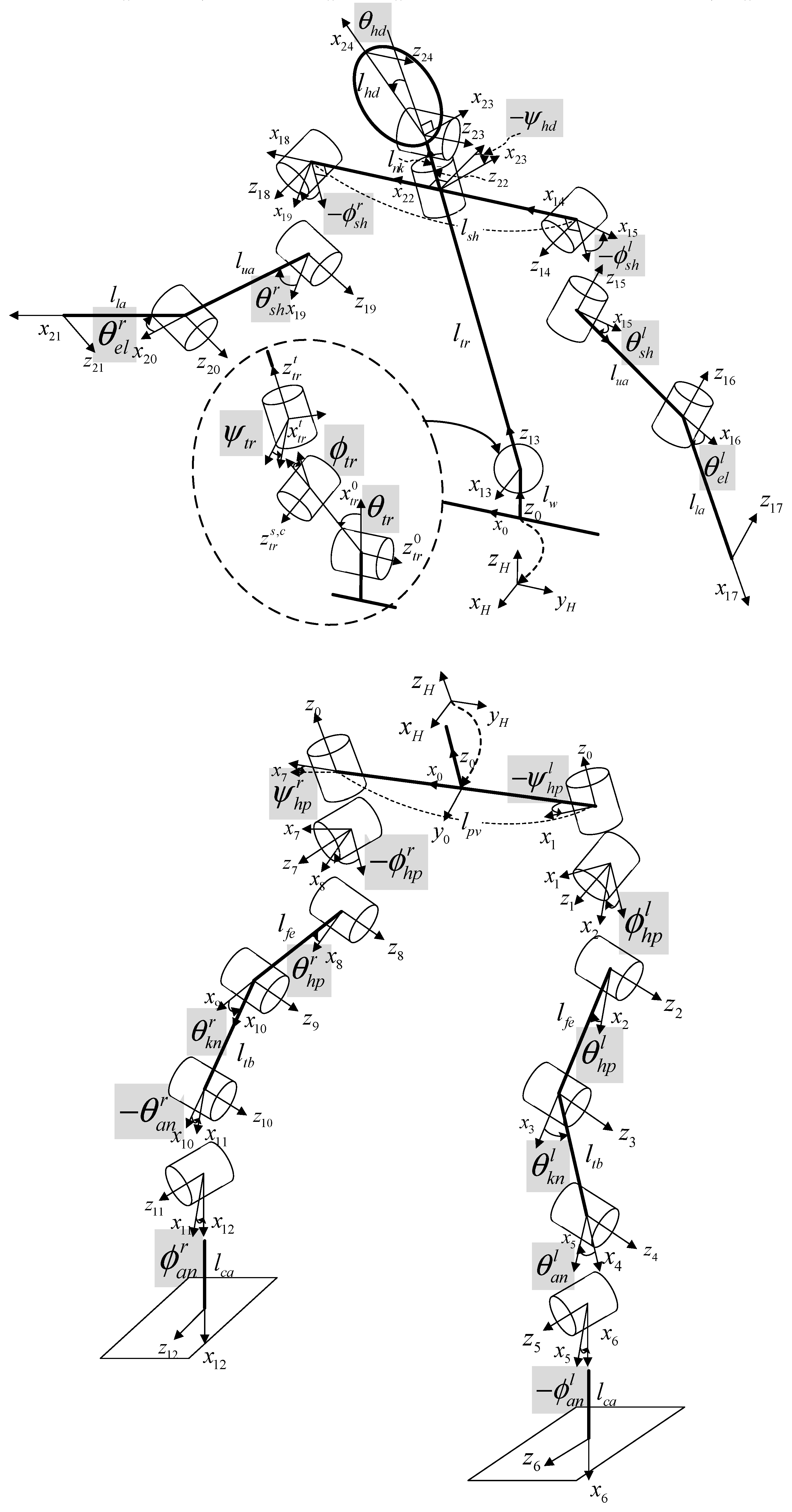
As shown in Figure 2, the proposed humanoid model is composed of a total of 23 joint variables. That is, it is composed of 12 joint angles which rotating axes are perpendicular to the sagittal plane ( θ h d , θ s h l , r , θ e l l , r , θ t r , θ h p l , r , θ k n l , r , θ a n l , r ) , 7 joint angles which rotating axes are perpendicular to the frontal plane ( ϕ s h l , r , ϕ t r , ϕ h p l , r , ϕ a n l , r ) , and 4 joint angles which rotating axes are perpendicular to the transverse plane ( ψ h d , ψ t r , ψ h p l , r ), where the subscripts hd, sh, el, tr, hp, kn, and an indicate joint names of the head, shoulder, elbow, torso, hip, knee, and ankle, respectively, and the superscripts l and r denote the left and right parts, respectively.

2.3. Reflecting Camera Effect

When deciding on a full-body pose, the position and viewing angle of the camera with respect to the subject are also crucial factors. The relative camera position determines the overall body size, which can be reflected to the humanoid model by multiplying the size factor γ to all the link lengths shown in Figure 2. That is, as the camera moves away, the body size decreases, i.e., γ < 1 , and vice versa, i.e., γ > 1 .
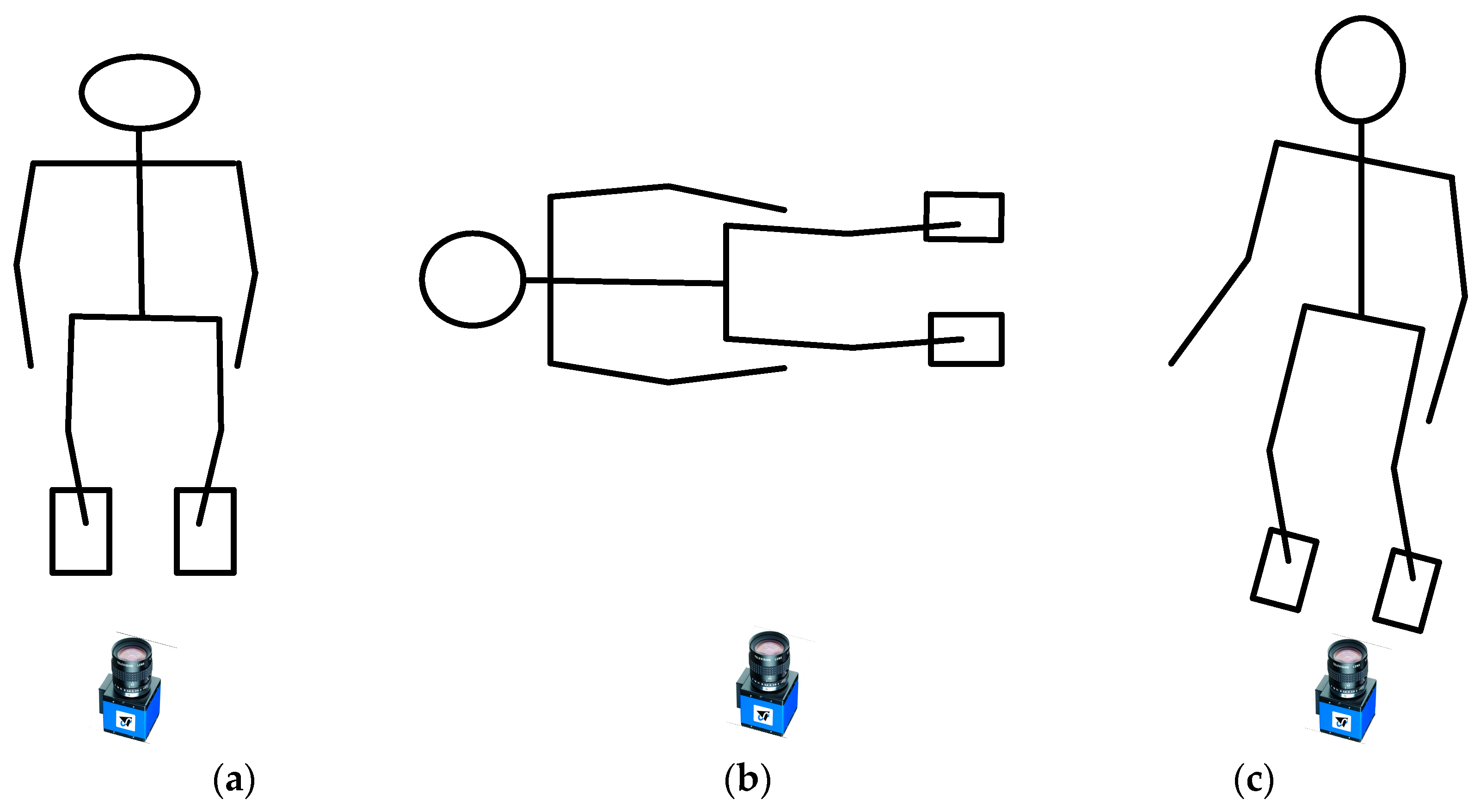
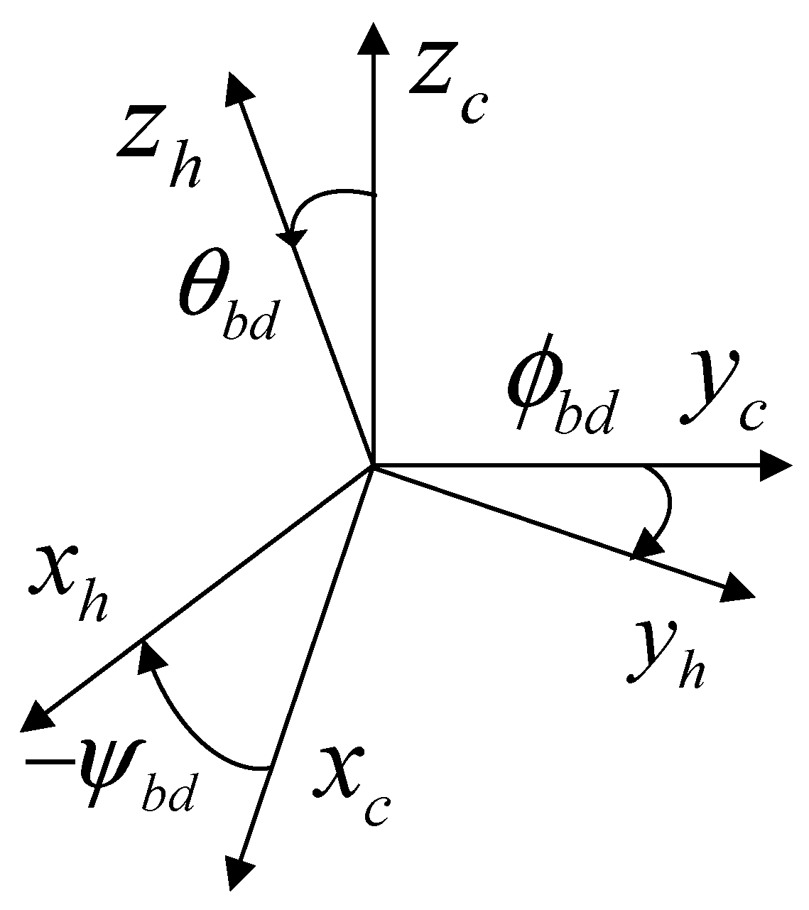
In addition, the relative camera view angle makes the same standing pose look different, as shown in Figure 3. Figure 3a shows a case where the camera shoots a subject from top to bottom. Figure 3b shows a situation where the camera is rotated 90 degrees clockwise. In Figure 3c, the camera views a subject from the front left. These differences in pose due to the camera view angle can be mathematically described by the relationship between the body coordinate frame and the camera-based coordinate frame, which is shown in Figure 4. The sagittal body angle θ b d , the coronal body angle ϕ b d , and the transversal body angle ψ b d correspond to the three pose changes in Figure 3, respectively. The polarity of these body angle parameters is determined to match the Vicon’s sign convention, such that θ b d > 0 for forward tilting, ϕ b d > 0 for left tilting, and ψ b d > 0 for left rotation [24], and vice versa.

2.4. Fast Global Optimization Method

For an estimation of the joint angles in the humanoid model that fits well with the MPP skeleton model for the current frame, inverse kinematics is basically necessary. However, it takes a long time to solve the formula-based inverse kinematics of the humanoid robot due to the complicated structure of the humanoid model, as shown in Figure 2.
uDEAS has been developed for solving non-smooth and multimodal engineering problems. uDEAS validates the fastest and most reliable global optimization performance on seven well-known low-dimensional (two to six) benchmark functions, three high-dimensional (up to 30) benchmark functions [29], the optimal designs of Gabor filter [30], and the joint trajectory generation for a humanoid’s ascending and descending stairs [31]. In addition, a modified version of uDEAS that can also search integer variables, cDEAS (combinatorial DEAS), has been recently developed and applied to the optimization of hybrid energy system [32].
uDEAS is a global optimization method that hybridizes local and global search schemes. For local search in uDEAS, all the optimization variables are represented by binary strings, such as genetic algorithm (GA) [33]. A basic unit of the local search is a session composed of single bisectional search (BSS) and multiple unidirectional search (UDS) with a binary string for each variable. The BSS attaches 0 and 1 at the end of the selected string as a new least significant bit (LSB), e.g., 010 2 01 2 011 2 , where the insertion of 0 (1) as a new LSB of the binary string corresponds to a decrease (increase) in its decoded real value compared to that of the parent string [23]. For example, assume that the binary string 010 2 is converted by the decoding function into a real value 0.3 and the cost value is 0.7, i.e., J ( d ( 010 2 ) ) = J ( 0.3 ) = 0.7 , whereas the binary string 011 2 is decoded into 0.1 and its cost value is 0.3, i.e., J ( d ( 011 2 ) ) = J ( 0.1 ) = 0.3 . Because J ( 0.1 ) < J ( 0.3 ) , increasing the current variable turns out to be a good search scheme as a result of the BSS.
On the other hand, the UDS adds or subtracts by 1 the optimal binary string according to the promising direction found at the previous BSS. For the BSS example mentioned above, the subsequent UDS will produce a binary string along the better BSS direction such that 100 2 ( first UDS ) 101 2 ( second UDS ) until no more cost reduction occurs. This set of BSS and UDS plays a significant role in balancing exploitation and exploration in the local search, respectively.
For the n-dimensional problem, uDEAS stacks up the n strings to make up a binary matrix with n rows.
  • Step 1. Initialization of new restart: Make an n × m binary matrix M which elements are randomly chosen binary digits. The row length index m is set m 0 . The optimization variable vector is v = [ v 1 v 2 v n ] T .
  • Step 2. Start the first session with i = 1 .
  • Step 3. BSS: From the current best matrix M , the binary vector of the j ( = J ( i ) ) -th row is selected as
    r j ( M ) = [ a j m a j ( m 1 ) a j 1 ] , a j k = { 0 , 1 } , 1 k m
    Attach 0 or 1 as a new LSB of the row vector, which yields
    r j = [ a j m a j ( m 1 ) a j 1 0 ] ,   r j + = [ a j m a j ( m 1 ) a j 1 1 ]
    Then, these strings are decoded into real values and replaced with the jth variable of the current best optimization variable vector v * as follows:
    v = v + = v * , v ( j ) = d ( r j ) , v + ( j ) = d ( r j + )
    Next, compute cost values J ( v ) and J ( v + ) . If J ( v ) < J ( v + ) , the direction for the UDS is set as u ( j ) = 1 ; otherwise, u ( j ) = 1 . The better row is saved as r j * .
  • Step 4. UDS: Depending on the direction u ( j ) , perform addition or subtraction to the jth row, which is described as
    r j ( M ) = r j * ( M ) + u ( j )
    Check whether the new row r j contributes to a further reduction of the loss function. If so, the current binary string and the variable are updated as the optimal ones as follows, and go to Step 4.
    r j * = r j , v * ( j ) = d ( r j * )
    Otherwise, go to Step 5.
  • Step 5. Save the resultant UDS best string, r * ( M ) , into the jth row of the current best matrix.
  • Step 6. If i < n , set i = i + 1 . Go to Step 3. Otherwise, if the current string length m is shorter than the prescribed maximal row length m f , set i = 1 , increase the row length index as m = m + 1 , and go to Step 2. In the case of m = m f , go to Step 7.
  • Step 7. If the number of restarts is less than the specified value, go to Step 1. Otherwise, terminate the current local search routine and choose the global minimum with the smallest cost value among the local minima found so far.

3. Proposed Pose Estimation Algorithm

Pose Estimation Process

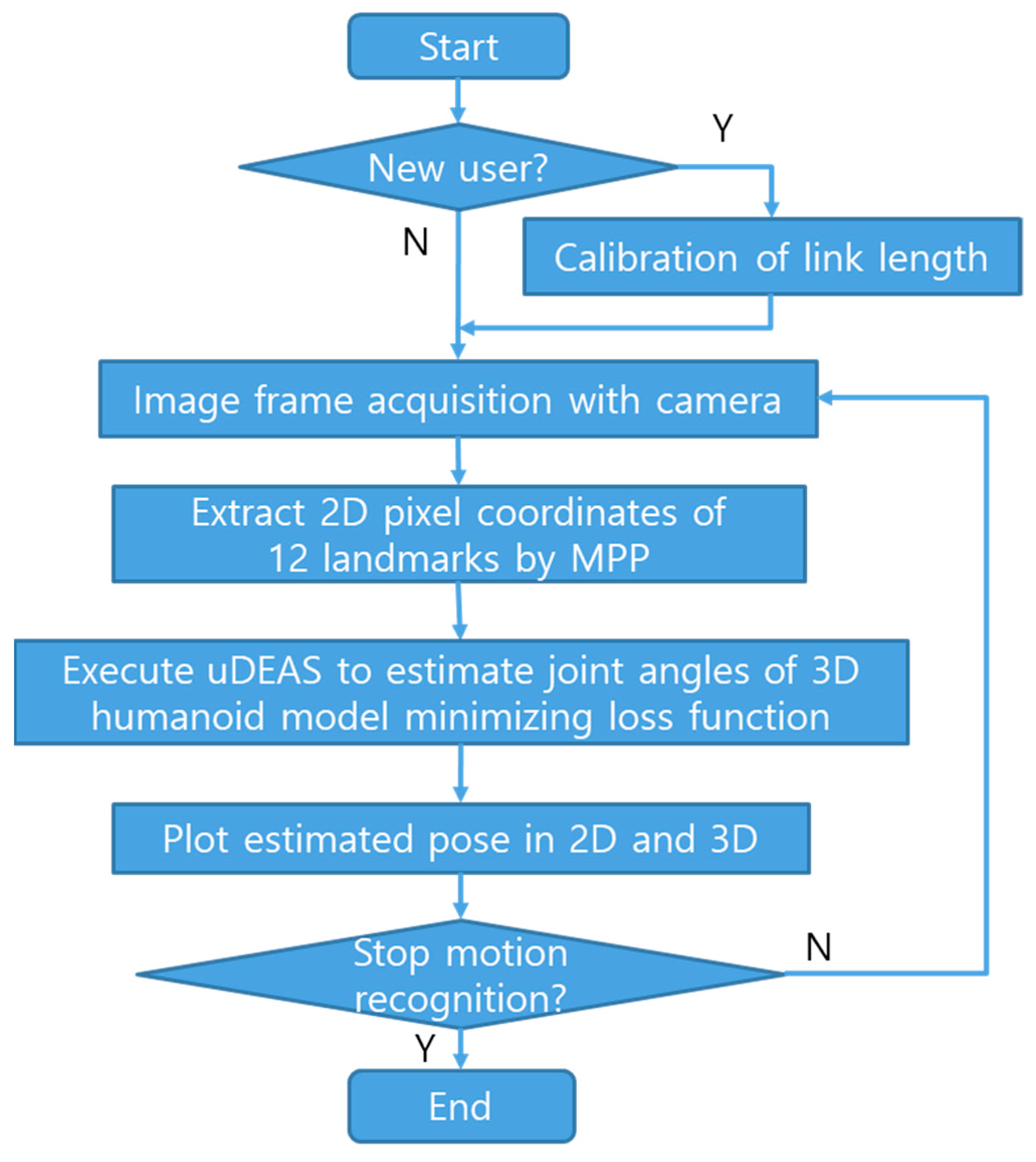
Figure 5 shows the overall flow diagram of the proposed pose estimation system.
  • Step 1. Calibration of link length: Our system checks whether the human subject is a new user or not because the subject’s bone length information is basically necessary for the model-based pose estimation. If the present system has no link length data for the current subject, the link length measurement process begins; the subject stands with the arms stretched down, images are captured for at least 10 frames, and the length of each bone link is calculated as the average distance between the coordinates of the end joints of the bone at each frame.
  • Step 2. Acquire images from an RGB camera with an image grabber module of SBC. Although an Intel RealSense camera is used in the present system, commercial RGB webcams are also available.
  • Step 3. Execute MPP and obtain 2D pixel coordinates of the 17 landmarks for the captured human body.
  • Step 4. Execute uDEAS to seek for unknown pose-relevant variables, such as the camera’s distance factor and viewing angles, and the intrabody joint angles by reducing the loss function formulated with the L2 norm between the joint coordinates obtained with MPP and those reprojected onto the corresponding 2D plane.
  • Step 5. Plot the estimated poses in 2D or 3D depending on the application field.
  • Step 6. If the current image frame is the last one or a termination condition is met, stop the pose estimation process. Otherwise, go to Step 2.
For an estimation of arbitrary poses at each frame, the size factor, γ , and the three body angle values related to the camera view angle, such as θ b d , ϕ b d , and ψ b d mentioned in Section 2.3, are added to the list of optimization variables. Therefore, a complete optimization vector for pose estimation consisting of 19 variables is estimated as follows:
V = [ γ , θ b d , ϕ b d , ψ b d , θ t r , ϕ t r , ψ t r , θ h p l , θ k n l , θ h p r , θ k n r , θ s h l , θ e l l , θ s h r , θ e l r , ϕ h p l , ϕ h p r , ϕ s h l , ϕ s h r ] T
The loss function to be minimized by uDEAS is designed to reflect three features: mean per joint position error (MPJPE) between the 2D MPP skeleton model and the fitted humanoid model; deviation of the 2D coordinates of the center of mass (CoM) from the center of the supporting feet of the 3D humanoid’s pose; and penalty values concerning the joint angles of the humanoid pose for consistency with the natural human pose.
The MPJPE is calculated by the mean distance between the true coordinates (for simulation case) or the MPP pixel coordinates (for experimental case), ( x p i , j , y p i , j ) and the coordinates of the 2D reprojected humanoid model onto the camera-based frame in Figure 4, ( y c i , j , z c i , j ) , which is described as
M P J P E ( v ) = ( x p i , j , y p i , j ) ( y c i , j , z c i , j ) 2 12 ,   i = l , r , j = s h , e l , w r , h p , k n , a n
When the two poses overlap exactly, this value decreases to zero.
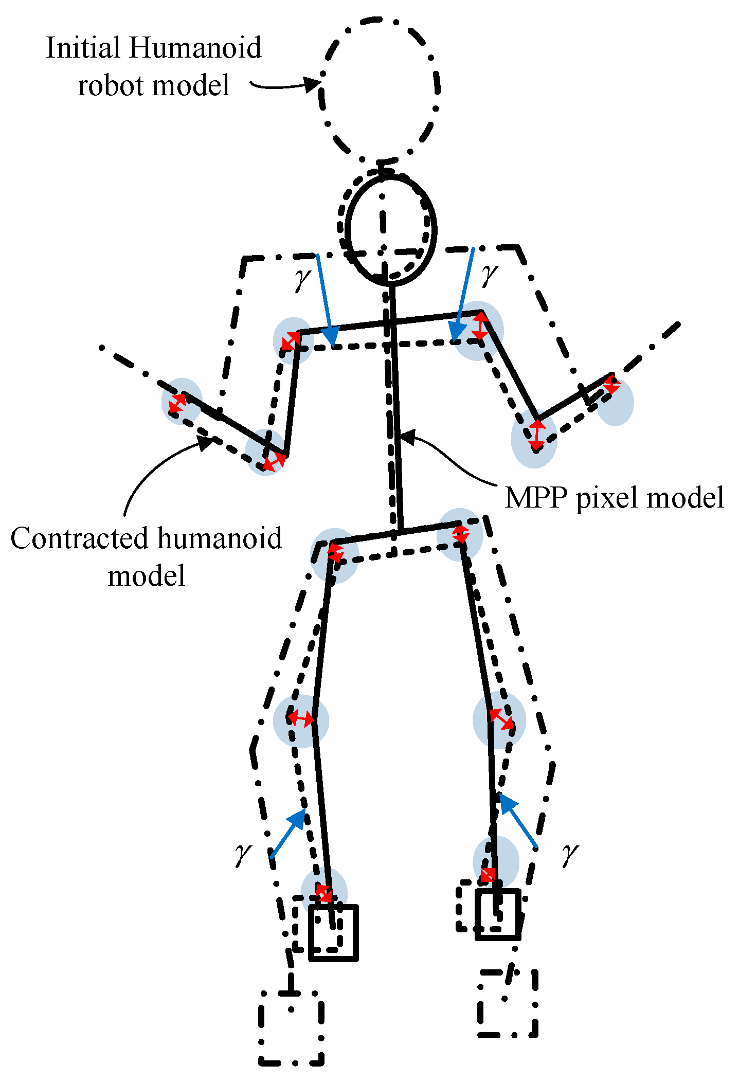
Figure 6 shows three models: the MPP pixel model, the initial humanoid model, and the tuned model, which pelvis centers are moved to the origin of the coordinate frame. uDEAS simultaneously adjusts the model contraction factor γ and the body and joint angles in Equation (7) to minimize the average deviation between the MPP pixel model and the contracted humanoid model in terms of the distance between the joint coordinates in the 2D plane, which is illustrated with red arrows.
The humanoid’s CoM deviation (CoMD) measured on the floor as the second pose metric is significant for measuring the standing stability of the current pose generated by uDEAS. Based on the camera-based coordinate frame x c y c z c defined in Figure 4, CoM D is described as follows:
C o M D ( v ) = ( x c C o M , y c C o M ) ( x c l , f t , y c l , f t ) + ( x c r , f t , y c r , f t ) 2 2 l l e g
where ( x c C o M , y c C o M ) is the coordinate of the humanoid’s CoM projected onto the floor; ( x c i , f t , y c i , f t ) , i = l , r denotes the center of the floor coordinates of the left and right feet; and l l e g denotes the length of the leg attained by summing the three links in the leg, i.e., l l e g = l f e + l t b + l c a , which is necessary for normalization.
As the third metric of loss function, penalty functions concerning the suitable bounds of some joint angles are newly proposed to make it possible to find the best fit among several identical 3D poses for an estimated MPP pose. Figure 7 shows three types of penalty functions for joint angles. The single-sided negative (positive) penalty function P s n ( P s p ) and the double-sided penalty function P d are defined as follows:
P s n ( θ , σ n ) = { | θ σ n | , θ < σ n 0 , θ σ n
P s p ( θ , σ p ) = { | θ σ p | , θ > σ p 0 , θ σ p
P d ( θ , σ n , σ p ) = { | θ σ n | , θ < σ n | θ σ p | , θ σ p 0 , σ n θ < σ p
where σ n and σ p represent negative and positive threshold values for joint angle θ , respectively. P s n ( P s p ) plays the role of informing uDEAS by increasing the loss function that an unrealistic pose is generated when a specific joint angle falls (increases) below (above) the assigned threshold angle. For example, when a human is standing, a sagittal torso angle θ t r smaller than 20 ° , i.e., leaning back, is rare, and thus adding P s ( θ t r , 20 ° ) to the loss function may prevent the generation of an unnatural pose by uDEAS. On the other hand, P d s is a useful function for creating the most realistic pose when a certain joint angle is within the two angles σ n and σ p . For instance, a sitting pose generally has the range of coronal torso angle ϕ t r between 10 ° and 10 ° , and thus adding P s ( ϕ t r , 10 ° , 10 ° ) to the loss function will help uDEAS select the feasible ϕ t r . The total loss function is formulated in Section 4.

4. Experimental Setup and Results

For the proposed human pose estimation system, Intel NUC 11th i7 (NUC11TNKi7) was used as the SBC for camera image acquisition and joint estimation, and Intel RealSense is installed as a commercial RGB-D sensor. In the SBC, the CPU is a quad-core i7-1165G7 (4.7 GHz) and the memory is 16 GB DDR4. The HDD is SSD NVMe 480 GB, and the OS is Ubuntu 18.04. For a high-mobility pose estimation capability, these modules are installed on a mobile robot base, as shown in Figure 8.
The basic configuration of uDEAS is determined as follows:
  • Number of optimization variables: 19.
  • Initial row length: 3.
  • Maximum row length: 12.
  • Number of maximum restarts: 20.
For pose estimation with a single image or an initial image of a video, the search ranges of each variable need to be determined appropriately, i.e., not too wide for search efficiency and not too narrow for inclusion of global minima. Table 1 summarizes the upper and lower bounds of the optimization variables in which all the joint variables can generate six ADL poses. In pose estimation with simulated poses where the ground-truth joint angles are known, the size factor is set as 1.0. Among the joint variables, the knee and elbow joints must have only positive angles, and, thus, their lower bounds are all set as zero.
For pose estimation with a sequence of images, the search ranges are adjusted around the optimal variables found by uDEAS in the previous image frame. In this paper, the upper limit of the optimization variable was determined by adding 10 degrees to the optimal variable of the previous frame, and the lower limit was set by subtracting 10 degrees from this. In this case, when the minimum rotation angle must be 0 degrees, such as the elbow or knee joint, care must be taken to ensure that the adjusted search’s lower limit does not fall below 0 degrees.

4.1. Pose Estimation with Simulation Data

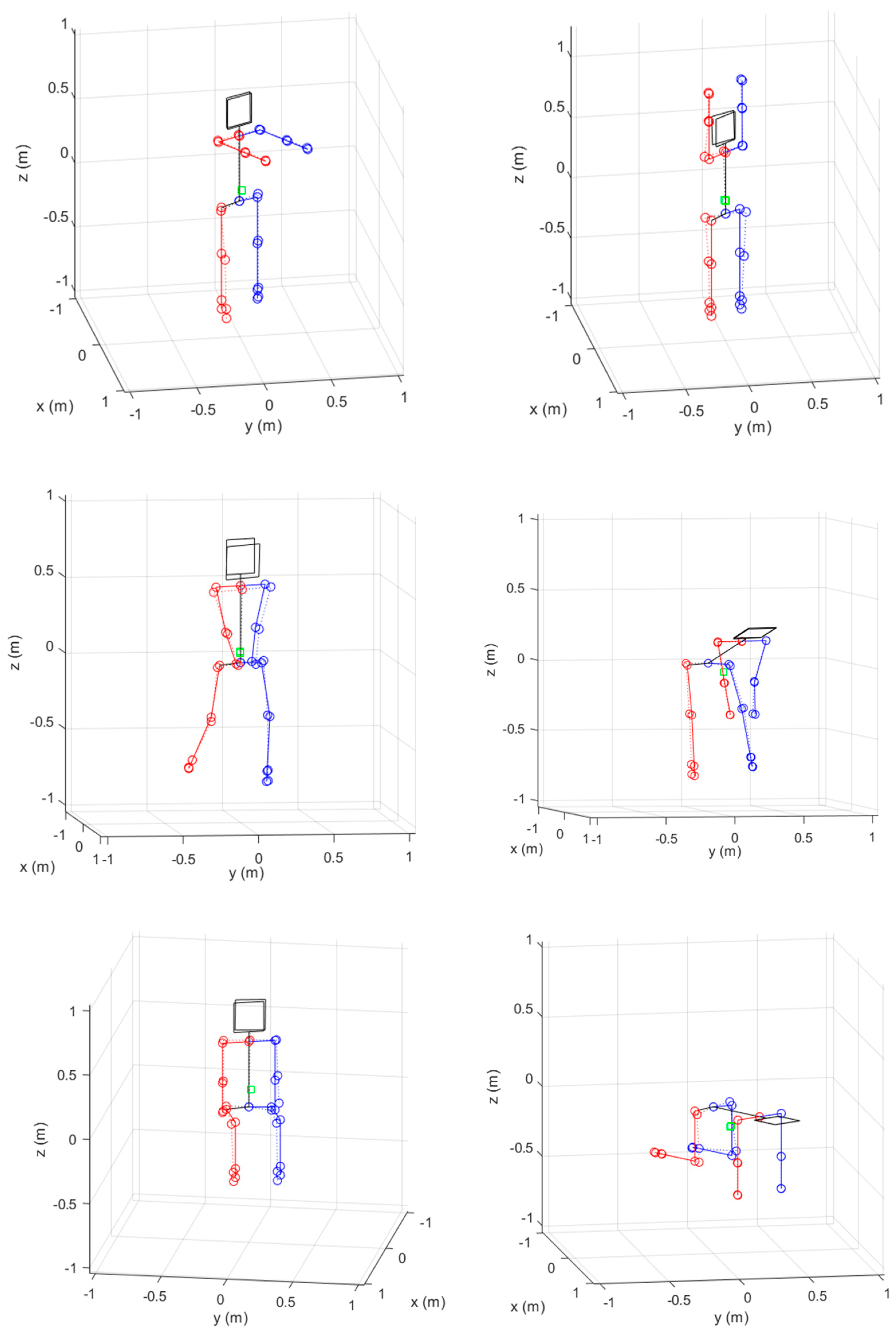
For the performance validation of the proposed approach, we generated six poses; (1) stand and raise arms front; (2) stand and raise arms up; (3) walk with the left leg in front; (4) bend down and grab an object; (5) sit on a chair; and (6) kneel down.
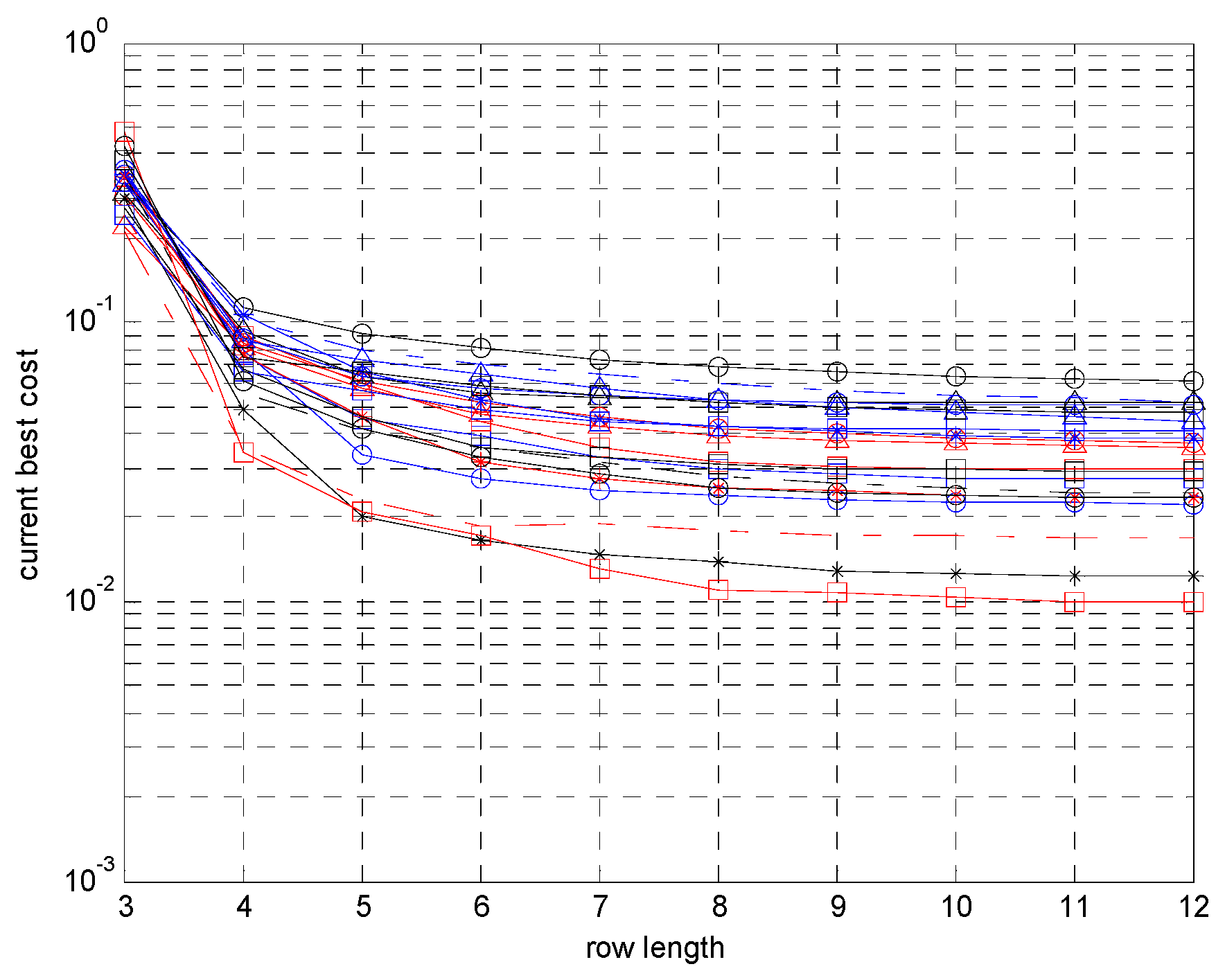
Figure 9 shows that the loss function profiles gradually minimize during 20 restarts for a given pose. It is apparent that the loss functions converge when the row length of the uDEAS matrices reach 10.
Figure 10 shows that uDEAS successfully estimates the six poses under the current optimization configuration. Table 2 lists the MPJPE of each global minimum in Equation (7), the average angular difference between the 18 ground-truth joint angles in Equation (6), and the estimated ones for the six poses. The average MPJPE is 0.097 m, and the average angle difference per joint is 10.017 degrees, which is an acceptable result for pose estimation with a full-scale humanoid model. The body size was selected referring to average Korean women in their twenties [34]. It is worth noting that all poses were created with the body transverse angles ( ψ b d ) between 20 and 40 degrees for generalization, which indicated that the camera view angle was set to the side of the subject.

4.2. Pose Estimation with Experiment

For the performance validation of the proposed pose estimation method, several activities in standing, sitting, and lying poses were filmed with an RGB camera and analyzed by our system.
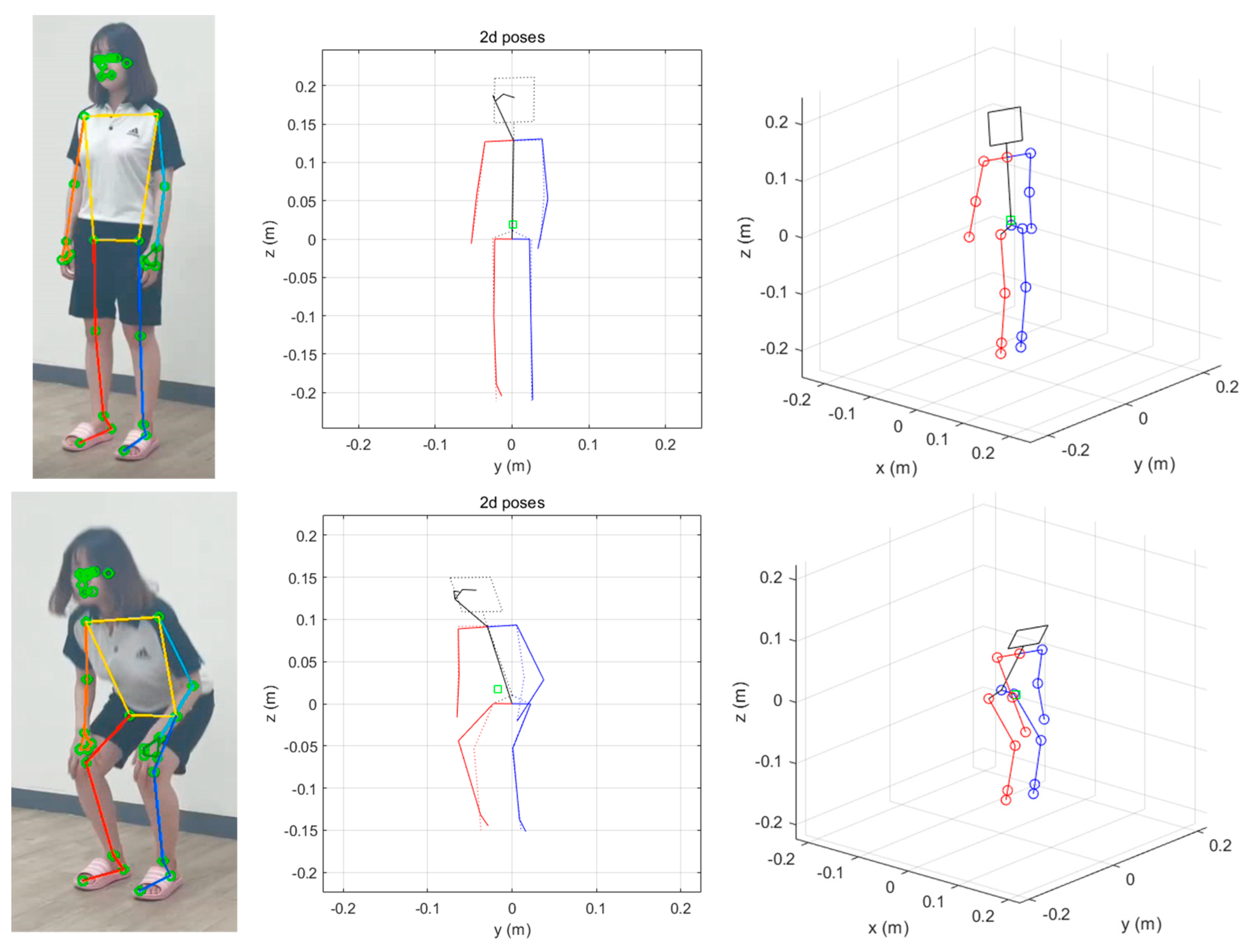
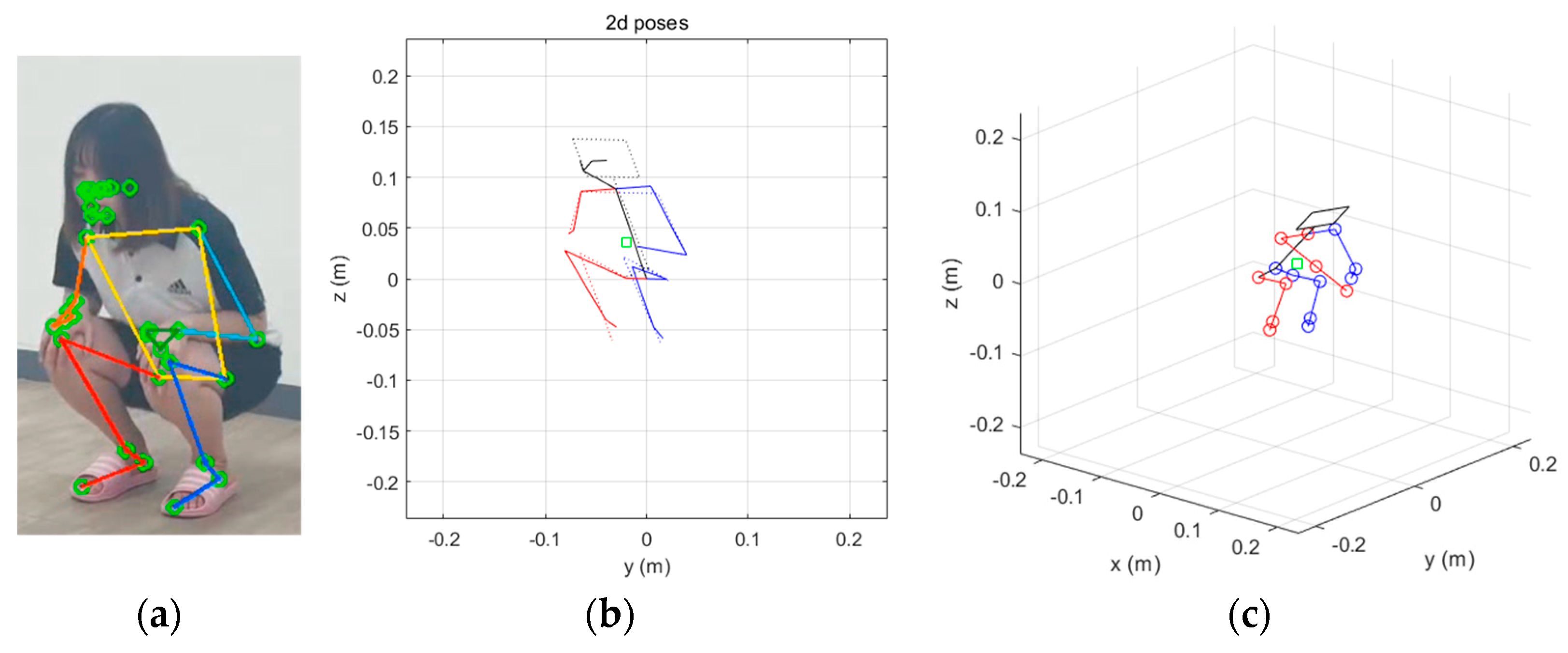
Figure 11 shows three poses captured and analyzed while standing and squatting. Figure 11a,b show the 2D poses estimated by MPP and the reprojected poses attained by uDEAS, and Figure 11c shows the reconstructed 3D poses.
The loss function needs to reflect the pose match, pose stability, pose symmetry, and penalty values for the joint angles of the torso and both shoulders as follows:
L ( v ) = M J C D ( v ) + γ C o M C o M D ( v ) + γ s y m ( | θ h p l θ h p r | + | θ k n l θ k n r | ) + γ s a g _ t r P s n ( θ t r , 10 ° ) + γ c o r _ t r P d ( ϕ t r , 10 ° , 10 ° ) + γ t r a n _ t r P d ( ψ t r , 15 ° , 15 ° ) + γ s a g _ s h _ l P s n ( θ s h l , 10 ° ) + γ s a g _ s h _ r P s n ( θ s h r , 10 ° ) + γ c o r _ s h _ l P s p ( ϕ s h l , 20 ° ) + γ c o r _ s h _ r P s p ( ϕ s h l , 20 ° )
where the weights γ C o M and γ c o r _ s h _ r denote the effects of each term on the loss function to reflect the adequacy of the reconstructed 3D pose. Because the MPJPE was in the order of 10 3 , these weights needed to be 0.01. The threshold values of the penalty functions can be selected appropriately for a target pose and activity.
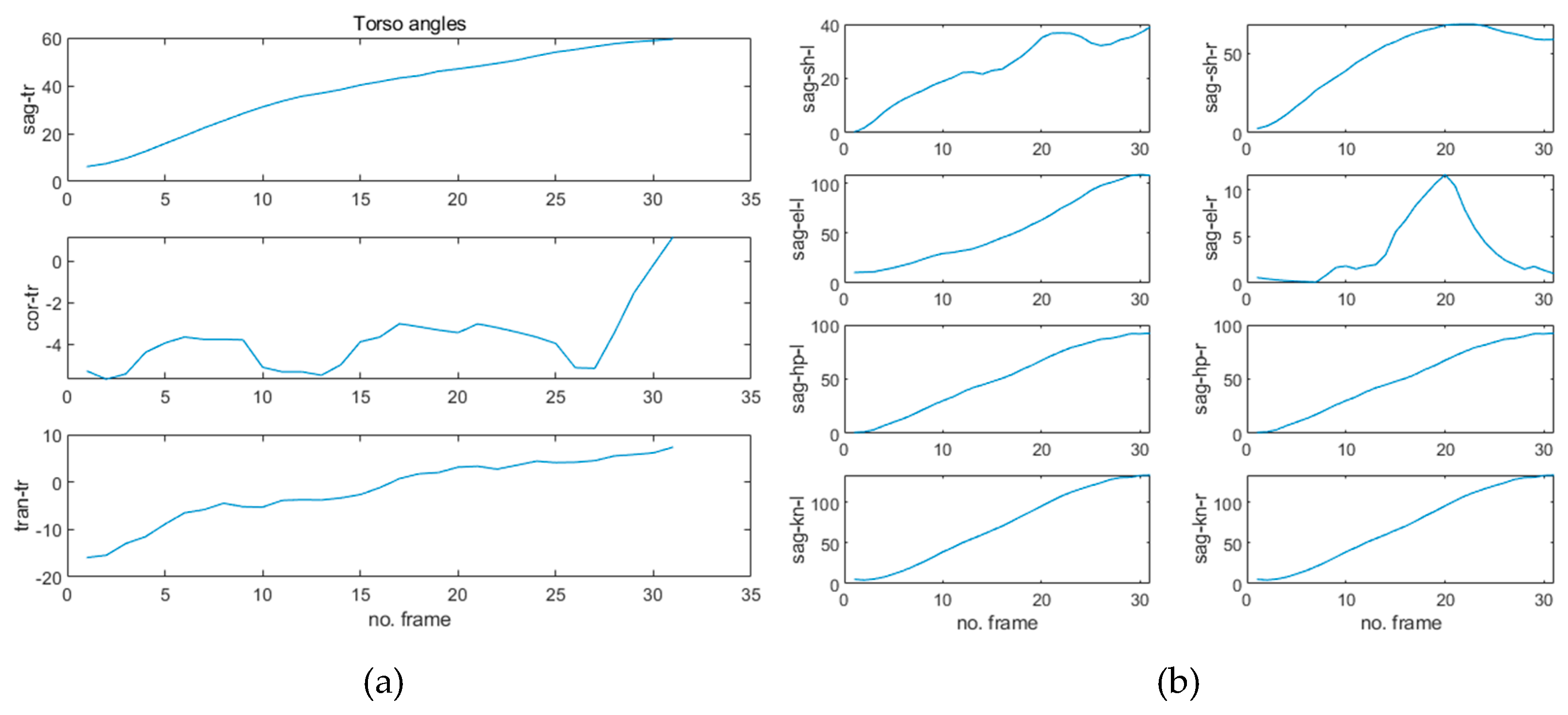
Figure 12 shows the trajectories of the estimated joint angles for the poses from Figure 11a–c. It is noteworthy that the sagittal hip and knee joints move from 0 to around 100 degrees, and the sagittal torso angles change from 0 to 60 degrees, which match the actual human joint angles rather well. These angle trajectories also provide information on the current stance, making them helpful for medical or therapeutic purposes.
For real-time application of the proposed pose optimization system, the execution time needs to be measured while running uDEAS on NUC. Table 3 lists the mean run time per frame measured while changing the number of restarts and the maximum row length of uDEAS. Interestingly, the optimal row length is found to be six when number of restarts is set at 10 because the loss of the next row length ( 7.22 × 10 3 ) increases significantly. In the same manner, the optimal number of restarts is 6 when the optimal row length is 12. As a combination of these results, the loss and mean run time per frame are 7.04 × 10 3 and 0.033 s, respectively, in the case when the number of restarts and the maximum row length are both six. Since this optimization execution time is below 100 ms, i.e., camera-capturing time for each frame at 10 fps, it is likely that real-time pose estimation is possible with the proposed system.
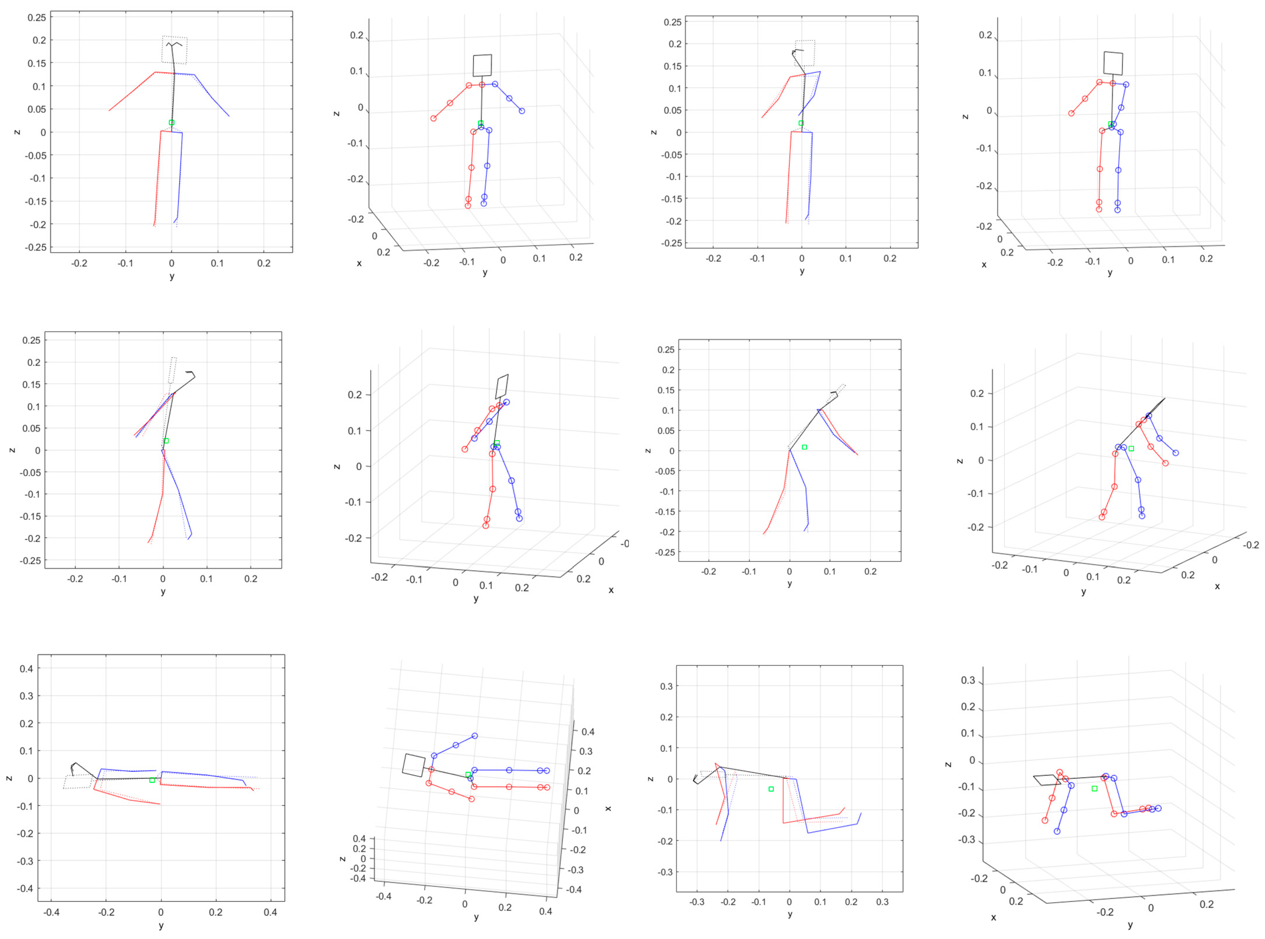
Figure 13 shows various 2D poses and the corresponding 3D poses reconstructed from the 2D poses using the camera images and MPP. It can be seen that the reconstructed humanoid models are similar to the actual 3D poses owing to the loss function that reflects many conditions related to the stable poses.
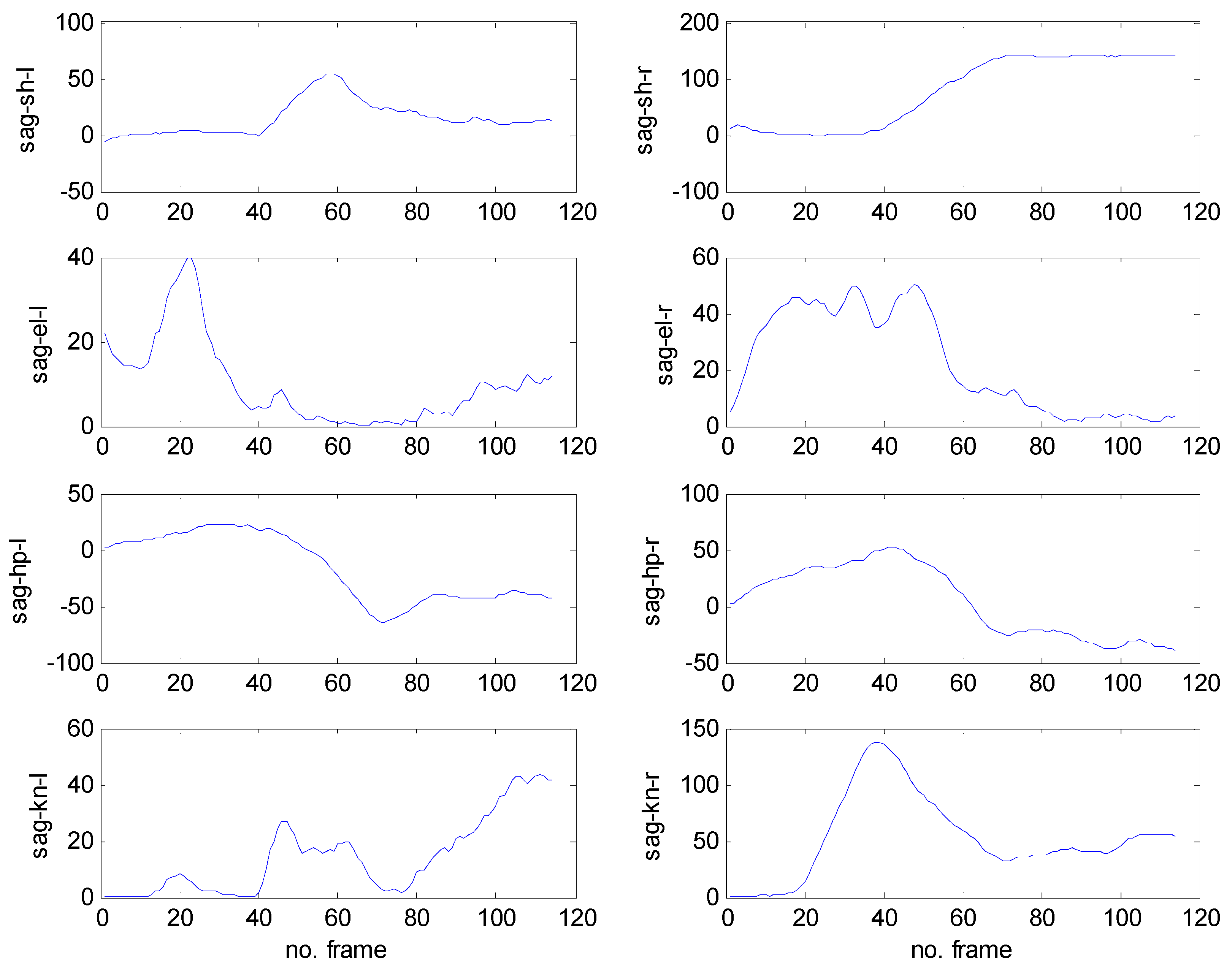
To verify the activity estimation performance, a sudden fall motion estimation was attempted, as shown in Figure 14 and Figure 15. The images captured in Figure 14 and the poses of the humanoid model in Figure 15 match well, and the estimated joint angle trajectories plotted in Figure 16 have apparently abnormal features. Specifically, the fact that the hip and knee joint angles in the sagittal plane change suddenly from 0 degree (standing) to 50 (hip) and 120 (knee) degrees means that the subject is instantly folding their right leg. As such, other poses can be recognized based on the representative joint angle profiles using the proposed approach.
Actually, MPP estimates the depth data for each landmark as well [22]. As a validation of the depth estimation performance of MPP, Figure 17 compares two 3D standing poses estimated by the proposed method and MPP. As shown in the figure, the depth data of each joint estimated by the current version of MPP have large errors when compared with our results. The ratio of the 2D MPJPE and 3D MPJPE is 185.37 for the standing pose and 277.81 for the arm-raised pose. The latter pose is more twisted than the former one from the camera’s viewpoint, and thus the depth error leads to a more different pose. This result is why we have employed only 2D landmark information for recovering 3D human pose estimation in the present work. Even if the depth value is estimated almost exactly in the later version of MPP, our method can be applied as it is, and the 3D estimation accuracy is expected to be higher.

5. Conclusions

In this paper, we present a 3D human pose estimation system from monocular images and videos by taking 2D skeletal poses estimated by the off-the-shelf deep learning method, MPP, as the input and fitting through reprojecting the 3D humanoid robot model to the 2D model at the joint angle level using the fast optimization method, uDEAS. Recently, most pose estimation methods are developed by using deep neural networks and, thus, require high-performance PCs or SBCs with many GPUs, which has limitation for application to mobile robot systems because of rapid heating issue and purchasing difficulties due to a lack of semiconductor supply chain. In order to improve the pose estimation performance, we elaborated our full-body humanoid robot model by adding three joints at the root joint and added a loss function CoM deviation term and penalty functions as constraints in the joint angle ranges for pose balance. Adopting the CoM concept is a novel idea in the area of pose estimation. With these efforts, the optimization execution time per frame is measured at 0.033 s on a NUC without GPU, showing the feasibility of a real-time system.
To validate the proposed approach, we generated 3D simulation data for six ADL poses and compared them with the poses estimated by uDEAS. The mean MPJPE was 0.097 m, and the average angle difference per joint was 10.017 degree, which is an acceptable result for pose estimation. The execution time of uDEAS was measured as 0.033 s in the case when the number of restarts and the maximum row length were both six, which was below the camera-capturing time of 0.1 s (10 fps); thus, it is likely that real-time pose estimation is possible with the proposed system. In the experiment with the proposed system, a standing to squatting activity, several whole-body exercises, and a dangerous activity of falling were captured on video, and each frame was input into the proposed system. The results show that very fast and drastic changes occur in the angular trajectories of the shoulder, elbow, hip, and knee joints, providing a lot of information for activity recognition. In future work, the proposed pose estimation system may be applied to analyze the activities of construction workers and to monitor patients with Parkinson’s disease to build a database of joint angles for human motions in target areas. It is expected that timely awareness of abnormal or dangerous activities will be possible based on direct joint angle information. In addition, the present approach without the use of deep learning model and dataset can complement deep learning-based methods in analyzing and recognizing arbitrary ADL poses.

Author Contributions

Software, J.-W.K., J.-Y.C. and E.-J.H.; Data curation, E.-J.H.; Writing—original draft, J.-W.K.; Funding acquisition, J.-H.C. All authors have read and agreed to the published version of the manuscript.

Funding

This research was funded by the National Research Foundation of Korea (NRF) with a grant funded by the Korea government (MSIT) (No. NRF-2021R1A4A1022059) and by the NRF grant funded by the MSIT (2020R1A2C1014649).

Informed Consent Statement

Informed consent was obtained from all subjects involved in the study.

Data Availability Statement

No new data were created or analyzed in this study. Data sharing is not applicable to this article.

Conflicts of Interest

The authors declare no conflict of interest.

References

  1. Su, M.; Hayati, D.W.; Tseng, S.; Chen, J.; Wei, H. Smart Care Using a DNN-Based Approach for Activities of Daily Living (ADL) Recognition. Appl. Sci. 2020, 11, 10. [Google Scholar] [CrossRef]
  2. Noreils, F.R. Inverse kinematics for a Humanoid Robot: A mix between closed form and geometric solutions. Tech. Rep. 2017, 1–31. [Google Scholar] [CrossRef]
  3. Yu, Y.; Yang, X.; Li, H.; Luo, X.; Guo, H.; Fang, Q. Joint-level vision-based ergonomic assessment tool for construction workers. J. Constr. Eng. Manag. 2019, 145, 04019025. [Google Scholar] [CrossRef]
  4. Rokbani, N.; Casals, A.; Alimi, A.M. IK-FA, a new heuristic inverse kinematics solver using firefly algorithm. Comput. Intell. Appl. Model. Control 2015, 369–395. [Google Scholar] [CrossRef] [Green Version]
  5. Xu, J.; Yu, Z.; Ni, B.; Yang, J.; Yang, X.; Zhang, W. Deep kinematics analysis for monocular 3d human pose estimation. In Proceedings of the IEEE/CVF Conference on Computer Vision and Pattern Recognition, Seattle, WA, USA, 13–19 June 2020; pp. 899–908. [Google Scholar]
  6. Li, J.; Xu, C.; Chen, Z.; Bian, S.; Yang, L.; Lu, C. Hybrik: A hybrid analytical-neural inverse kinematics solution for 3d human pose and shape estimation. In Proceedings of the IEEE/CVF Conference on Computer Vision and Pattern Recognition, Nashville, TN, USA, 19–25 June 2021; pp. 3383–3393. [Google Scholar]
  7. Sarafianos, S.; Boteanu, B.; Ionescu, B.; Kakadiaris, I.A. 3D human pose estimation: A review of the literature and analysis of covariates. Comput. Vis. Image Underst. 2016, 152, 1–20. [Google Scholar] [CrossRef]
  8. Chen, Y.; Tian, Y.; He, M. Monocular human pose estimation: A survey of deep learning-based methods. Comput. Vis. Image Underst. 2020, 192, 102897. [Google Scholar] [CrossRef]
  9. Wang, J.; Tan, S.; Zhen, X.; Xu, S.; Zheng, F.; He, Z.; Shao, L. Deep 3D human pose estimation: A review. Comput. Vis. Image Underst. 2021, 210, 103225. [Google Scholar] [CrossRef]
  10. Yurtsever, M.M.E.; Eken, S. BabyPose: Real-time decoding of baby’s non-verbal communication using 2D video-based pose estimation. IEEE Sens. 2022, 22, 13776–13784. [Google Scholar] [CrossRef]
  11. Alam, E.; Sufian, A.; Dutta, P.; Leo, M. Vision-based human fall detection systems using deep learning: A review. Comput. Biol. Med. 2022, 146, 105626. [Google Scholar] [CrossRef]
  12. Pavlakos, G.; Zhou, X.; Derpanis, K.G.; Daniilidis, K. Coarse-to-fine volumetric prediction for single-image 3D human pose. In Proceedings of the IEEE Conference on Computer Vision and Pattern Recognition, Honolulu, HI, USA, 21–26 July 2017; pp. 7025–7034. [Google Scholar]
  13. Luvizon, D.C.; Picard, D.; Tabia, H. 2d/3d pose estimation and action recognition using multitask deep learning. In Proceedings of the IEEE Conference on Computer Vision and Pattern Recognition, Salt Lake City, UT, USA, 18–22 June 2018; pp. 5137–5146. [Google Scholar]
  14. Li, S.; Chan, A.B. 3d human pose estimation from monocular images with deep convolutional neural network. In Proceedings of the Asian Conference on Computer Vision, Singapore, 1–5 November 2014; pp. 332–347. [Google Scholar]
  15. Zhou, X.; Sun, X.; Zhang, W.; Liang, S.; Wei, Y. Deep kinematic pose regression. In Proceedings of the European Conference on Computer Vision, Amsterdam, The Netherlands, 11–14 October 2016; pp. 186–201. [Google Scholar]
  16. Tome, D.; Russell, C.; Agapito, L. Lifting from the deep: Convolutional 3d pose estimation from a single image. In Proceedings of the IEEE Conference on Computer Vision and Pattern Recognition, Honolulu, HI, USA, 21–26 July 2017; pp. 2500–2509. [Google Scholar]
  17. Wang, J.; Huang, S.; Wang, X.; Tao, D. Not all parts are created equal: 3D pose estimation by modelling bi-directional dependencies of body parts. arXiv 2019, arXiv:1905.07862. [Google Scholar]
  18. Wandt, B.; Rosenhahn, B. Repnet: Weakly supervised training of an adversarial reprojection network for 3d human pose estimation. In Proceedings of the IEEE/CVF Conference on Computer Vision and Pattern Recognition, Long Beach, CA, USA, 16–20 June 2019; pp. 7782–7791. [Google Scholar]
  19. Sigal, L.; Balan, A.O.; Black, M.J. Humaneva; Synchronized video and motion capture dataset and baseline algorithm for evaluation of articulated human motion. IJCV 2010, 87, 4–27. [Google Scholar] [CrossRef]
  20. Ionescu, C.; Papava, D.; Olaru, V.; Sminchisescu, C. Human3.6m: Large scale datasets and predictive methods for 3d human sensing in natural environments. TPAMI 2014, 36, 1325–1339. [Google Scholar] [CrossRef] [PubMed]
  21. Pavllo, D.; Feichtenhofer, C.; Grangier, D.; Auli, M. 3D human pose estimation in video with temporal convolutions and semi-supervised training. In Proceedings of the IEEE Conference on Computer Vision and Pattern Recognition, Long Beach, CA, USA, 16–20 June 2019; pp. 7753–7762. [Google Scholar]
  22. MediaPipe Pose. Available online: https://google.github.io/mediapipe/solutions/pose.html (accessed on 28 December 2021).
  23. Kim, J.-W.; Kim, T.; Park, Y.; Kim, S.W. On load motor parameter identification using univariate dynamic encoding algorithm for searches (uDEAS). IEEE Trans. Energy Convers. 2008, 23, 804–813. [Google Scholar]
  24. Vicon. Available online: https://www.vicon.com/ (accessed on 1 August 2021).
  25. Vakanski, A.; Jun, H.P.; Paul, D.; Baker, R. A data set of human body movements for physical rehabilitation exercises. Data 2018, 3, 2. [Google Scholar] [CrossRef] [PubMed] [Green Version]
  26. Bazarevsky, V.; Grishchenko, I. On-Device, Real-Time Body Pose Tracking with MediaPipe BlazePose, Google Research. Available online: https://ai.googleblog.com/2020/08/on-device-real-time-body-pose-tracking.html (accessed on 10 August 2021).
  27. Denavit, J.; Hartenberg, R.S. A kinematic notation for lower-pair mechanisms based on matrices. J. Appl. Mech. 1955, 77, 215–221. [Google Scholar] [CrossRef]
  28. Kim, J.-W.; Tran, T.T.; Dang, C.V.; Kang, B. Motion and walking stabilization of humanoids using sensory reflex control. Int. J. Adv. Robot. Syst. 2016, 13, 1–10. [Google Scholar]
  29. Kim, J.-W.; Kim, T.; Choi, J.-Y.; Kim, S.W. On the global convergence of univariate dynamic encoding algorithm for searches (uDEAS). Int. J. Control Autom. Syst. 2008, 6, 571–582. [Google Scholar]
  30. Yun, J.P.; Choi, S.; Kim, J.-W.; Kim, S.W. Automatic detection of cracks in raw steel block using Gabor filter optimized by univariate dynamic encoding algorithm for searches (uDEAS). NDT E Int. 2009, 42, 389–397. [Google Scholar] [CrossRef]
  31. Kim, E.; Kim, M.; Kim, S.-W.; Kim, J.-W. Trajectory generation schemes for bipedal ascending and descending stairs using univariate dynamic encoding algorithm for searches (uDEAS). Int. J. Control Autom. Syst. 2010, 8, 1061–1071. [Google Scholar] [CrossRef]
  32. Kim, J.-W.; Ahn, H.; Seo, H.C.; Lee, S.C. Optimization of Solar/Fuel Cell Hybrid Energy System Using the Combinatorial Dynamic Encoding Algorithm for Searches (cDEAS). Energies 2022, 15, 2779. [Google Scholar] [CrossRef]
  33. Goldberg, D.E. Genetic Algorithm in Search, Optimization and Machine Learning; Addison Wesley: Berkeley, CA, USA, 1999. [Google Scholar]
  34. Size Korea. Available online: https://sizekorea.kr (accessed on 15 March 2022).
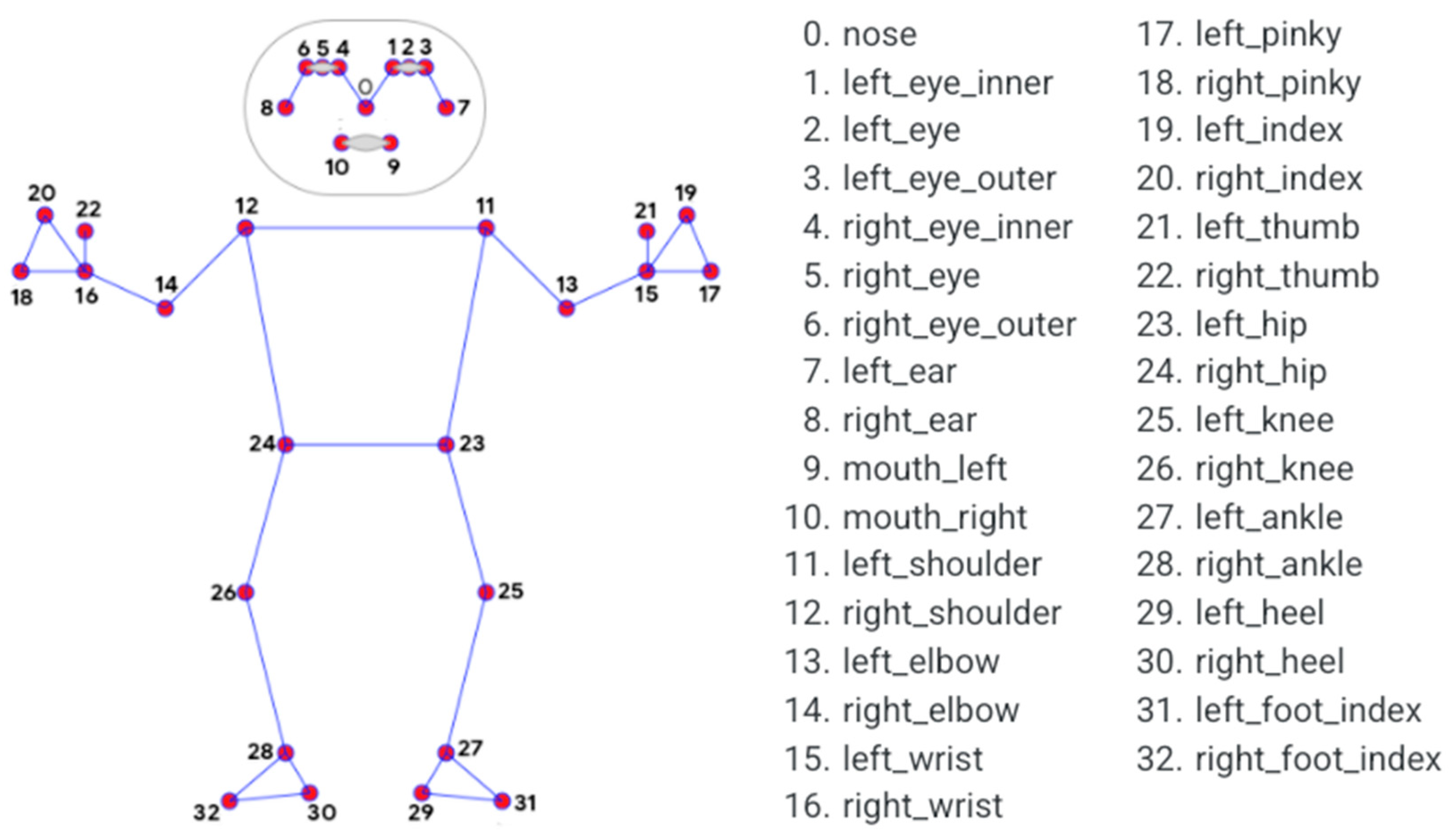
Figure 1. Definition of landmarks in MediaPipe Pose [22].
Applsci 13 02700 g001
Figure 2. The 3D humanoid robot model.
Applsci 13 02700 g002
Figure 3. Identical poses looking different according to the camera view angles. (a) from top to bottom, (b) rotated 90 degrees clockwise, (c) from the front left.
Applsci 13 02700 g003
Figure 4. Relationship between the body coordinate fame, x h y h z h , and the camera-based coordinate frame, x c y c z c .
Applsci 13 02700 g004
Figure 5. Flow diagram of the proposed pose estimation process.
Applsci 13 02700 g005
Figure 6. Pose comparison in the 2D frontal plane between the MPP pixel model (solid line) and the fitted model (dashed line) contracted from the initial humanoid model (dash-dotted line).
Applsci 13 02700 g006
Figure 7. Penalty functions for suitable joint angles. (a) single-sided negative function, (b) single-sided positive function, and (c) double-sided function.
Applsci 13 02700 g007
Figure 8. Human pose recognition system.
Applsci 13 02700 g008
Figure 9. Minimization aspect of loss function during 20 restarts of uDEAS with each restart colored differently.
Applsci 13 02700 g009
Figure 10. Pose estimation results for the six representative poses generated by the humanoid model (solid line: true pose, dotted line: estimated pose, red line: right parts, blue line: left parts).
Applsci 13 02700 g010
Figure 11. Pose estimation results for three poses generated by the humanoid model. (a) Original images and MPP results overlaid, (b) comparison between the MPP model (solid line) and the fitted humanoid model (dotted line) in 2D plane, and (c) the humanoid model reconstructed in 3D plane (red line: right parts, blue line: left parts).
Applsci 13 02700 g011aApplsci 13 02700 g011b
Figure 12. Trajectories of the estimated joint angles (degree) at (a) the torso and (b) the sagittal plane.
Applsci 13 02700 g012
Figure 13. Two-dimensional poses and the corresponding 3D poses reconstructed by the proposed approach viewed from various angles (red line: right parts, blue line: left parts).
Applsci 13 02700 g013aApplsci 13 02700 g013b
Figure 14. Results of 2D pose estimation obtained by MPP for a sequence of images in a sudden falling case (red line: right parts, blue line: left parts).
Applsci 13 02700 g014aApplsci 13 02700 g014b
Figure 15. Results of the reconstructed 3D humanoid poses corresponding to Figure 13 (red line: right parts, blue line: left parts).
Applsci 13 02700 g015
Figure 16. Angular trajectories (in degrees) of the shoulder, elbow, hip, and knee joints in the sagittal plane.
Applsci 13 02700 g016
Figure 17. Comparison of 3D poses obtained from MPP (solid) and the proposed approach (dotted). (a) standing pose, (b) arm-raised pose (red line: right parts, blue line: left parts).
Applsci 13 02700 g017
Table 1. Upper and lower bounds of the optimization variables (in degrees).
γ θ b d ϕ b d ψ b d θ t r ϕ t r ψ t r θ h p l θ k n l θ h p r θ k n r θ s h l θ e l l θ s h r θ e l r ϕ h p l ϕ h p r ϕ s h l ϕ s h r
V ¯ 110109090403090909090180901809040404040
V _ 1−10−10−90−20−40−30−200−200−1800−1800−40−40−40−40
Table 2. MPJPE and average angular difference values for the best-fitted poses in Figure 10.
Pose123456Avg.
MPJPE (m)0.00550.00990.01110.00490.01500.01160.097
Avg. ang. diff (deg)6.0617.74810.5575.614.55815.5810.017
Table 3. Comparison of uDEAS run time measured in NUC (bold: optimal configuration).
No. RestartMax. Row Length Loss   ( × 10 3 ) Avg. Run Time Per Frame (s)
10126.520.180
116.630.165
106.630.137
96.540.118
86.740.096
76.720.078
66.940.062
57.220.044
412.890.028
9126.650.170
86.730.149
76.680.130
66.980.113
57.150.096
47.980.079
667.040.033
Disclaimer/Publisher’s Note: The statements, opinions and data contained in all publications are solely those of the individual author(s) and contributor(s) and not of MDPI and/or the editor(s). MDPI and/or the editor(s) disclaim responsibility for any injury to people or property resulting from any ideas, methods, instructions or products referred to in the content.