Adaptive Dynamic Programming-Based Cross-Scale Control of a Hydraulic-Driven Flexible Robotic Manipulator

Featured Application

The proposed method is suitable for application in robotic arm systems.

Abstract

This paper focuses primarily on adaptive dynamic programming (ADP)-based tracking control of the hydraulic-driven flexible robotic manipulator system (HDFRMS) with varying payloads and uncertainties via singular perturbation theory (SPT). Firstly, the dynamics is derived using a driven Jacobin matrix, which represents the coupling between the hydraulic servo-driven system and rigid–flexible manipulator established using the assumed mode method and Lagrange principle. Furthermore, the whole dynamic model of the manipulator system is decoupled into a second slow subsystem (SSS), a second fast subsystem (SFS) and a first fast subsystem (FFS). The three subsystems can describe a large range of movement, flexible vibration and electro-hydraulic servo control, respectively. Hereafter, an adaptive dynamic programming trajectory tracking control law with a critic-only policy iteration algorithm is presented in the second slow timescale, while both robust optimal control (ROC) in the second first timescale and adaptive sliding mode control (ASMC) in the first fast timescale are also designed using the Lyapunov stability theory. Finally, the numerical simulations are carried out to illustrate the rightness and robustness of the singular perturbation decomposition and proposed composite control algorithm.

1. Introduction

The hydraulic-driven flexible robotic manipulator system (HDFRMS) has wide implementation potentials in a large number of engineering fields human can hardly deal with directly, such as forest exploitation, heavy payload motion control, construction work, mobile equipment applications and other industrial areas [1,2,3], since their energy consumption and weight are lower, but the speed is higher.

Unlike rigid manipulators, the dynamics of flexible manipulators is the nonlinear rigid–flexible coupling infinite-order model [4,5]. Indeed, many control methods have been presented for flexible multibody dynamics system, in particular flexible link manipulators and flexible joint manipulators, involving PID control [6,7], neural network control [8], sliding mode control [9], adaptive control [10], optimal control [11], etc. Nevertheless, ill-conditioned numerical issues and inaccurate or unreliable control will occur, because these dynamic model-based control methods are directly designed ignoring multiple timescales in dynamics. Singular perturbation theory (SPT) is used to deal with the problem of control under different timescales.

The two-order dynamic model of flexible systems can be decoupled into the slow subsystem (SS) in slow timescale, which is the traditional timescale, and the fast subsystem (FS) in new timescale, namely fast timescale based on SPT. In [4,12] the flexible link manipulator system is decomposed through the perturbation parameter that the small-time constant is defined as, and two sub-controllers are designed. The composite control consisting of fuzzy sliding mode control in SS and linear quadratic regulator (LQR) optimal control in FS are proposed in [13]. Additionally, in [14], the slow controller is substituted by the learning controller and the disturbance observer to improve the trajectory tracking precision. An adaptive non-saturated control is preferentially considered to handle actuator saturation involving dynamics parameters in the flexible joint manipulator system, where there are any parametric uncertainties [4,15]. Additionally, the adaptive neural backstepping control in SS is presented as the uncertain nonlinearity compensator [16]. Furthermore, the fuzzy control [17], the robust fuzzy sliding mode control [18] and the adaptive high-gain Kalman filter [19] are investigated to improve robustness.

Compared with the electrical-driven manipulator, hydraulic-driven manipulators have higher power to handle heavier payloads whose weights are greater than 100 kg, and they have lower stiffness and response time. However, the order of their dynamic equations that are more complicated is raised from the second order to the third order. It is so difficult to control them because of electro-hydraulic coupling and inherent elastic vibration. A hybrid controller including a feedforward control and feedback control [20], and model-based adaptive energy shaping controller [21] are proposed in the hydraulic manipulator system. Many observers, such as the adaptive observer and variable structure disturbance observer, are also designed to handle uncertainties and vibrations [22,23,24]. However, the description of dynamics is not complete yet. That is, flexible vibration or hydraulic drive has always been ignored in past controller designs. Therefore, the control method which can track desired trajectories precisely and suppress flexible vibrations based on the complete electro-hydraulic coupling model needs be presented.

In the work, we discuss an ADP-based trajectory tracking control law and singular perturbation decoupling for the HDFRMS with uncertainties and varying payloads. The main contributions include the following three aspects.

(1) The whole third-order dynamic model including three link rigid–flexible manipulator, asymmetric four-way valve controlled hydraulic cylinder and hydraulic actuator is derived. It is more beneficial and complete than the actual engineering system, since both the flexible vibration and hydraulic drive are considered in the dynamic model.

(2) A novel singular perturbation decoupling method for the electro-hydraulic servo flexible multibody dynamics system is presented. Unlike the traditional method that contains one perturbation parameter and two timescales, two singular perturbation parameters are used to establish three timescales.

(3) An optimal control method based on the critic-only policy iteration algorithm for tracking control is proposed, which simplifies the controller structure of ADP. The controller can improve the control precision and optimize the energy consumption, because the model network and control network of traditional ADP are not considered.

The rest of the paper is organized as follows. We derive the whole dynamics of the manipulator system in Section 2. Three decoupled subsystems are obtained based on SPT in Section 3. Section 4 presents two tasks that are the design of composite control scheme and the closed-loop stability analysis at the same time. Some simulation results are exhibited in Section 5. Finally, Section 6 draws some conclusions.

2. Dynamic Modeling of HDFRMS

We consider the mechanical structure involving the first rigid link with a rotary joint, the second rigid link with a revolute joint and the last flexible link with another revolute joint (see Figure 1).

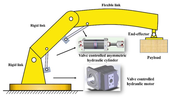
Figure 1. Model of HDFRMS.

2.1. Mechanical Subsystem Model

Link 1 and 2 of HDFRMS are rigid. However, the third link, like a slender beam, is flexible. Its vibration will occur because the end-effector with heavy payload and manipulator system have large overall motions. Only the transverse vibration is considered, except for the axial deformation and shear deformation. Therefore, the Euler–Bernoulli beam theory is sufficient to describe the flexible deformation and vibration of the third link.

Concretely, the dynamic modeling of HDFRMS consists of two parts: mechanical subsystem modeling and hydraulic subsystem modeling.

We derive the dynamics of the mechanical subsystem using vibration analysis result-based AMM via Lagrange’s equation. The following assumptions are made based on the actual situation. Table 1 shows the nomenclature of the mechanical subsystem.

Table 1. Notation, frequently used symbols of mechanical subsystem.

Symbol	Definition	Symbol	Definition
$L_i$	length of ith link	$r_1$	upper surface radius of link 1
${\theta }_i$	angle of ith joint	$r_2$	lower surface radius of link 1
$m_i$	mass of the ith actuator	$M$	mass of payload
${\rho }_i$	mass density per unit length of ith link	$EI$	elastic stiffness
$L_{11}$$L_{21}$	installation location of the first hydraulic cylinder	$\omega (r,t)$	elastic deformation of flexible link 3
$L_{22}$$L_{31}$	installation location of the second hydraulic cylinder	${\mathsf{\Phi }}_j(r)$	jth mode shape function of flexible link 3
$g$	acceleration of gravity	$q_j(t)$	jth modal displacement of flexible link 3

Assumption 1.

The payload is held tightly by the manipulator end-effector, and their contact is static.

Assumption 2.

The mass of actuators focuses on joints of the manipulator.

Let $XOY$ and $X_{i}O{Y}_i$ be the inertial Cartesian coordinate and the moving coordinates fixed on the robotic manipulator, respectively. Figure 2 illustrates the schematic diagram of four primary coordinate systems for HDRMES.

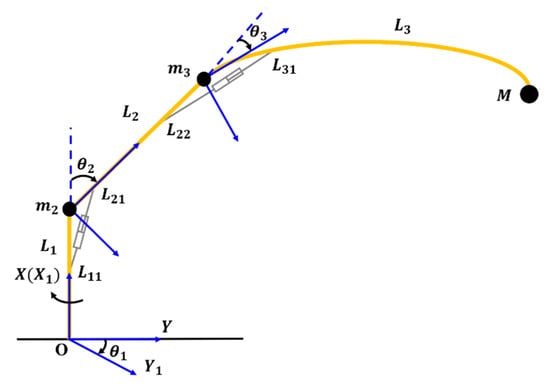
Figure 2. Schematic diagram of rigid–flexible manipulator.

Considering AMM, we find the elastic displacement $\omega (r,t)$ of the third link as:

$$\omega (r,t) = {\displaystyle \sum _{j=1}^n{\mathsf{\Phi }}_j(r)q_j(t)}$$

(1)

The higher order modes are ignored, and only previous order modes are considered in practical engineering application, because they can make greater impacts on system performances.

When flexible link 3 is conceived as cantilever beam model, one end of this link is supported simply, and the other end is free [6]. Therefore, we can obtain the elastic displacement

$$\omega (r,t) = {\mathsf{\Phi }}_1(r)q_1(t)+{\mathsf{\Phi }}_2(r)q_2(\mathrm{T})$$

(2)

$${\mathsf{\Phi }}_j(r) = sh{\beta }_{j}r + {\zeta }_j\sin {\beta }_{j}r$$

(3)

where ${\zeta }_j = sh{\beta }_j{L}_3/\sin {\beta }_j{L}_3$, ${\beta }_j = (j+0.25)\pi /L_3$, $j = 1,2$. $r$ is position of any point on the third link, and $0 \le r \le L_3$.

Considering the coordinate system and the kinematics of three link rigid–flexible manipulators, the kinetic energy of the mechanical subsystem can be obtained as

$$\begin{array}{cc}\hfill T& =(\frac{1}{6}{\rho }_2{L}_2^3+\frac{1}{2}{m}_3{L}_2^2+\frac{1}{2}{\rho }_3{L}_3{L}_2^2+\frac{1}{2}M{L}_2^2)({\dot{\theta }}_2^2+s_2^2{\dot{\theta }}_1^2)+[\frac{1}{6}{\rho }_1(r_2^3-r_1^3)+\frac{1}{2}{m}_2{r}_1^2]{\dot{\theta }}_1^2\hfill \\ & +{\rho }_3{L}_2{\displaystyle {\int }_0^{L_3}\dot{\omega }dr}{\dot{\theta }}_2{c}_3+\frac{1}{2}M{L}_3^2[{({\dot{\theta }}_2+{\dot{\theta }}_3)}^2+{\dot{\theta }}_1^2{s}_{23}^2]+\frac{1}{2}{\rho }_3{\displaystyle {\int }_0^{L_3}{\dot{\omega }}^{2}dr}+(\frac{1}{2}{\rho }_3{L}_2{L}_3^2\hfill \\ & +M{L}_2{L}_3)[c_3{\dot{\theta }}_2({\dot{\theta }}_2+{\dot{\theta }}_3)+s_2{s}_{23}{\dot{\theta }}_1^2]+(\frac{1}{2}{\rho }_3{\displaystyle {\int }_0^{L_3}{\omega }^{2}dr}+\frac{1}{2}M{\omega }_{L_3}^2)[{({\dot{\theta }}_2+{\dot{\theta }}_3)}^2+c_{23}^2{\dot{\theta }}_1^2]\hfill \\ & +L_2({\rho }_3{\displaystyle {\int }_0^{L_3}\omega dr}+M{\omega }_{L_3})[s_2{c}_{23}{\dot{\theta }}_1^2-s_3{\dot{\theta }}_2({\dot{\theta }}_2+{\dot{\theta }}_3)]+({\rho }_3{\displaystyle {\int }_0^{L_3}\dot{\omega }rdr}+M{L}_3{\dot{\omega }}_{L_3})({\dot{\theta }}_2+{\dot{\theta }}_3)\hfill \\ & +\frac{1}{2}M{\dot{\omega }}_{L_3}^2+({\rho }_3{\displaystyle {\int }_0^{L_3}\omega rdr}+M{L}_3{\omega }_{L_3})s_{23}{c}_{23}{\dot{\theta }}_1^2+M{L}_2{\dot{\omega }}_{L_3}{\dot{\theta }}_2{c}_3+\frac{1}{6}{\rho }_3{L}_3^3[{({\dot{\theta }}_2+{\dot{\theta }}_3)}^2+{\dot{\theta }}_1^2{s}_{23}^2]\hfill \end{array}$$

(4)

Including the elastic potential energy of flexible link 3, gravitational potential energy of manipulators and payloads, the potential energy of the mechanical subsystem can be derived as

$$\begin{array}{cc}\hfill V& =(\frac{1}{2}{\rho }_1{L}_1+{\rho }_2{L}_2+{\rho }_3{L}_3+m_2+m_3+M)g{L}_1+(\frac{1}{2}{\rho }_2{L}_2+{\rho }_3{L}_3+m_3+M)g{L}_2{c}_2\hfill \\ & +\frac{1}{2}EI{\displaystyle \underset{0}{\overset{L_3}{\int }}{\left\{\frac{{\partial }^2\omega }{\partial r^2}\right\}}^{2}dr}+(Mg{L}_3+\frac{1}{2}{\rho }_{3}g{L}_3^2-{\rho }_{3}g{\displaystyle {\int }_0^{L_3}\omega dr})c_{23}-Mg{\omega }_{L_3}{s}_{23}\hfill \end{array}$$

(5)

where $c_1=\cos {\theta }_1$, $c_2=\cos {\theta }_2$, $c_3=\cos {\theta }_3$, $s_1=\sin {\theta }_1$, $c_{23}=\cos ({\theta }_2+{\theta }_3)$, $s_3=\sin {\theta }_3$, $s_2=\sin {\theta }_2$, $s_{23}=\sin ({\theta }_2+{\theta }_3)$, $\omega =\omega (r,t)$, $\dot{\omega }={\mathsf{\Phi }}_1(r){\dot{q}}_1(t)+{\mathsf{\Phi }}_2(r){\dot{q}}_2(t)$, ${\dot{\omega }}_{L_3}={\mathsf{\Phi }}_1(L_3){\dot{q}}_1(t)+{\mathsf{\Phi }}_2(L_3){\dot{q}}_2(t)$ and $\frac{{\partial }^2\omega }{\partial r^2}={\ddot{\mathsf{\Phi }}}_1(r)q_1(t)+{\ddot{\mathsf{\Phi }}}_2(r)q_2(t)$.

Defining a Lagrange function $L$, which consists of total potential energy $V$ and total kinetic energy $T$, we get $L=T-V$.

According to the following Lagrange equation [25]

$$\frac{d}{d\mathrm{T}}(\frac{\partial L}{\partial {\dot{p}}_i})-\frac{\partial L}{\partial p_i}={\tau }_i$$

(6)

the dynamic model of the rigid–flexible manipulator without the viscous damping and the external interference can be expressed as

$$M(\theta ,q)\left[\begin{array}{c}\ddot{\theta }\\ \ddot{q}\end{array}\right]+K\left[\begin{array}{c}\theta \\ q\end{array}\right]+G(\theta ,\dot{\theta },q,\dot{q})=\left[\begin{array}{c}\tau \\ 0\end{array}\right]$$

(7)

where $M(\theta ,q)$ is the $5\times 5$ positive definite, symmetric, time-varying generalized inertia matrix, $K=diag(k_1,k_2)$ is the stiffness matrix of the flexible link 3, $G(\theta ,\dot{\theta },q,\dot{q})=$ ${[g_1{g}_2{g}_3{g}_4{g}_5]}^{\mathrm{T}}$ consists of Coriolis force, centrifugal force and gravity, $\theta = {[{\theta }_1{\theta }_2{\theta }_3]}^{\mathrm{T}}$ is the joint angles, $q = {[q_1{q}_2]}^{\mathrm{T}}$ is the mode coordinates and $\tau = {[{\tau }_1{\tau }_2{\tau }_3]}^{\mathrm{T}}$ is the control torque.

Remark 1.

Utilizing the Lagrange equation, p contains joint angles$\theta$ and elastic displacement $\omega$. The joint angles $\theta$and control torque $\tau$are considered when $i=1,2,3$. Otherwise, we have

$$\frac{d}{d\mathrm{T}}(\frac{\partial L}{\partial \dot{\omega }})-\frac{\partial L}{\partial \omega } = 0$$

2.2. Hydraulic Subsystem Model

Joint 1 is a rotary joint, which is driven by a rotary hydraulic motor. Joints 2 and 3 are revolute joints, which are driven by a linear asymmetric hydraulic cylinder. The manipulator needs to move the payload along some predefined trajectory in practice.

The hydraulic-driven subsystem consists of a hydraulic cylinder and hydraulic motor. Additionally, Table 2 shows the nomenclature of the hydraulic subsystem. The asymmetric four-way valve-controlled hydraulic cylinder is a kind of hydraulic actuator converting hydraulic energy into linear motion mechanical energy as shown in Figure 3.

Table 2. Notation, frequently used symbols of hydraulic subsystem.

Symbol	Definition	Symbol	Definition
$P_s$	supply pressure	$x_v$	spool displacement
$P_r$	return pressure	$y$	piston displacement
$P_L$	payload pressure	$L$	hydraulic cylinder stroke
${\beta }_e$	bulk modulus	$w$	area gradient of the valve
$C_d$	flow coefficient of the serve-valve port	$I$	servo valve current
$V_t$	equivalent volume	$K_q$	flow gain coefficient
$K_c$	flow/pressure coefficient	$Q_L$	load flow of hydraulic cylinder/motor
$P_1$ $P_2$	left and right actuator chamber pressure	$Q_1$ $Q_2$	left and right actuator chamber fluid flow
$D$	volume displacement of the motor	$V_1$ $V_2$	left and right actuator chamber volume
$C_{tm}$	equivalent leakage coefficient	$A_1$ $A_2$	left and right effective piston area

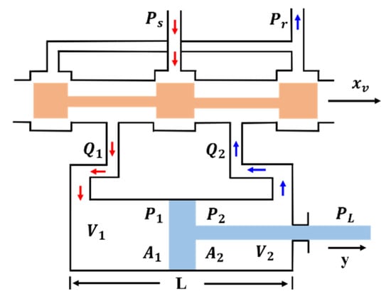
Figure 3. Schematic diagram of asymmetric hydraulic cylinder.

Actually, the time constant of mechanical systems is much greater than the hydraulic serve-valve time constant; therefore, the servo valve spool displacement $x_v$ is proportional to the control input by ignoring the dynamics of the servo valve. We obtain $K_i = K_v{K}_a$, where $K_v$ is the proportional valve gain and $K_a$ is the amplifier gain.

$$x_v = K_{i}i$$

(8)

Considering the law of cosines, depending on the installation location of hydraulic cylinder, we have

$$\begin{gathered} y_2 = \sqrt{L_{21}^2+L_{11}^2-2L_{11}{L}_{21}\cos (180-{\theta }_2)} \\ {y}_3 = \sqrt{L_{22}^2+L_{31}^2-2L_{22}{L}_{31}\cos (180-{\theta }_3)} \\ \dot{y} = J\dot{\theta } \end{gathered}$$

(9)

where $J = diag(J_1,J_2)$ is the matrix relating the actuator linear displacement to the link angular displacement.

Additionally, the details of this matrix $J$ are described below.

$$\begin{gathered} J_2 = \frac{\partial y_2}{\partial {\theta }_2} = \frac{-L_{21}{L}_{11}\sin {\theta }_2}{\sqrt{L_{21}^2+L_{11}^2+2L_{11}{L}_{21}\cos {\theta }_2}} \\ {J}_3 = \frac{\partial y_3}{\partial {\theta }_3} = \frac{-L_{22}{L}_{31}\sin {\theta }_3}{\sqrt{L_{22}^2+L_{31}^2+2L_{22}{L}_{31}\cos {\theta }_3}} \end{gathered}$$

(10)

According to the relationships of force balances and the basic theory of the hydraulic system [26], we obtain

$$\left\{\begin{array}{c}{Q}_L=K_q{x}_v-K_c{P}_L\hfill \\ Q_L=C_{tm}{P}_L+\frac{V_t}{4{\beta }_e}{\dot{P}}_L+A_p\dot{y}\hfill \\ x_v=K_{i}I\hfill \\ \tau =A_{p}J{P}_L\hfill \end{array}\right.A_p=\left\{\begin{array}{l}{A}_1{x}_v\ge 0\\ A_2{x}_v<0\end{array}\right.$$

(11)

Applying (9) and (11), we can derive that

$$\dot{\tau }+[\frac{4{\beta }_e}{V_t}(K_c+C_{tm})-\frac{\dot{J}}{J}]\tau +\frac{4{\beta }_e{A}_p^2}{V_t}{J}^2\dot{\theta }=\frac{4{\beta }_e{A}_p{K}_q{K}_i}{V_t}JI$$

(12)

where $V_t = 2L{A}_p^4/(A_1^3+A_2^3)$.

Similarly, the kinetics of the valve-controlled hydraulic motor can be derived as

$$\left\{\begin{array}{l}{x}_v=K_{i}I\\ \tau =P_{L}D\\ Q_L=K_q{x}_v-K_c{P}_L\\ Q_L=D\dot{\theta }+C_{tm}{P}_L+\frac{V_t}{4{\beta }_e}{\dot{P}}_L\end{array}\right.$$

(13)

where $K_q = C_{d}w\sqrt{(P_s-P_L)/\rho }$.

By simple calculation of (13), we can obtain the relationship between current and torque as follows.

$$\dot{\tau }+\frac{4{\beta }_e}{V_t}(C_{tm}+K_c)\tau +\frac{4{\beta }_e{D}^2}{V_t}\dot{\theta } = \frac{4{\beta }_{e}D{K}_q{K}_i}{V_t}I$$

(14)

From (12) and (14), the model of the hydraulic subsystem can be given as

$$\dot{\tau } + A\tau + B\dot{\theta } = CI$$

(15)

From the previous derivations, both (7) and (9) are the dynamic model of the HDFRMS.

$$\left\{\begin{array}{l}M(\theta ,q)\left[\begin{array}{c}\ddot{\theta }\\ \ddot{q}\end{array}\right]+K\left[\begin{array}{c}\theta \\ q\end{array}\right]+G(\theta ,\dot{\theta },q,\dot{q})=\left[\begin{array}{c}\tau \\ 0\end{array}\right]\hfill \\ \hfill \dot{\tau }+A\tau +B\dot{\theta }=CI\hfill \end{array}\right.$$

(16)

3. Cross-Scale Decoupling of Manipulator System

The dynamic model of the HDFRMS is essentially a strongly coupled third-order time-varying nonlinear differential equation. Therefore, it makes system control law design more difficult. In addition to this, it is difficult to guarantee system control performances due to the coupling when there are uncertainties and disturbances in system.

In this section, the complete dynamics for HDFRMS will be decomposed twice for control design based on singular perturbation. They are second slow subsystem, second fast subsystem and fast subsystem, respectively.

3.1. First Singular Perturbation Decomposition

Firstly, the complete dynamic model can be decoupled into the first stage SS that characterizes the rigid–flexible manipulator, as well as the first stage FS characterizing the hydraulic servo-driven part.

Defining the first singular perturbation parameter ${\epsilon }_1 = \raisebox{1ex}{$1$}\!\left/ \!\raisebox{-1ex}{${\beta }_e$}\right.$, it satisfies $0<{\epsilon }_1<<1$. Then, the dynamic model (16) can be rewritten as

$$\left\{\begin{array}{l}M(\theta ,q)\left[\begin{array}{c}\ddot{\theta }\\ \ddot{q}\end{array}\right]+K\left[\begin{array}{c}\theta \\ q\end{array}\right]+G(\theta ,\dot{\theta },q,\dot{q})=\left[\begin{array}{c}\tau \\ 0\end{array}\right]\hfill \\ {\epsilon }_1\dot{\tau }=-\tilde{A}\tau -\tilde{B}\dot{\theta }+\tilde{C}I\hfill \end{array}\right.$$

(17)

where $\tilde{A}={\epsilon }_{1}A$, $\tilde{B}={\epsilon }_{1}B$, $\tilde{C}={\epsilon }_{1}C$.

When perturbation parameter ${\epsilon }_1$ is small enough, the higher order infinitesimal $o\left({\epsilon }_1\right)$ can be ignored. According to multiple timescale theories, the variables $\tau$ and $I$ can be represented as

$$\begin{gathered} \tau = {\tau }_{f1}+{\tau }_{s1} \\ I = I_{f1} + I_{s1} \end{gathered}$$

(18)

where subscript $f1$ and subscript $s1$ represent the first level of fast timescales and slow timescales, respectively.

Setting ${\epsilon }_1 = 0$, we obtain the first stage SS, namely FSS

$$\left\{\begin{array}{l}M(\theta ,q)\left[\begin{array}{c}\ddot{\theta }\\ \ddot{q}\end{array}\right]+K\left[\begin{array}{c}\theta \\ q\end{array}\right]+G(\theta ,\dot{\theta },q,\dot{q})=\left[\begin{array}{c}{\tau }_{s1}\\ 0\end{array}\right]\hfill \\ {\tau }_{s1}=-{\tilde{A}}^{-1}\tilde{B}\dot{\theta }+{\tilde{A}}^{-1}\tilde{C}{I}_{s1}\hfill \end{array}\right.$$

(19)

We now introduce the first level of fast timescale ${\sigma }_1$ in the boundary layer, and we have

$${\sigma }_1 = \frac{t}{{\epsilon }_1}$$

(20)

The first-level slow variable ${\tau }_{s1}$ is considered constant near the boundary layer ${\epsilon }_1\to 0$. According to (17) and (19), the first stage FS, namely FFS, can be expressed as

$$\frac{d{\tau }_{f1}}{d{\sigma }_1} = -\tilde{A}{\tau }_{f1} + \tilde{C}{I}_{f1}$$

(21)

3.2. Second Singular Perturbation Decomposition

The FSS (19) will be decoupled again. We can have the SSS characterizing the large overall motion of the manipulator without the whole flexibilities, and the SFS is only about the flexible vibration of the third link.

We define the inverse matrix $D$ of matrix $M$ as

$$D = M^{-1} = \left[\begin{array}{c}{M}_1{M}_2\\ M_3{M}_4\end{array}\right]=\left[\begin{array}{c}{D}_1{D}_2\\ D_3{D}_4\end{array}\right]$$

(22)

where $M_1\in R^{3\times 3}$, $D_1\in R^{3\times 3}$.

Additionally, we make

$$G(\theta ,\dot{\theta },q,\dot{q}) = \left[\begin{array}{l}{G}_1\hfill \\ G_2\hfill \end{array}\right]$$

(23)

Substituting (22) and (23) into the first stage of the slow subsystem (19), we can obtain

$$\begin{array}{ll}\hfill \ddot{\theta }=& -D_2(\theta ,q)K_{x}q-D_1(\theta ,q)G_1(\theta ,\dot{\theta },q,\dot{q})-D_2(\theta ,q)G_2(\theta ,\dot{\theta },q,\dot{q})\hfill \\ & +D_1(\theta ,q)\left(-{\tilde{A}}^{-1}\tilde{B}\dot{\theta }+{\tilde{A}}^{-1}\tilde{C}{I}_{s1}\right)\hfill \end{array}$$

(24)

$$\begin{array}{ll}\hfill \ddot{q}=& -D_4(\theta ,q)K_{x}q-D_3(\theta ,q)G_1(\theta ,\dot{\theta },q,\dot{q})-D_4(\theta ,q)G_2(\theta ,\dot{\theta },q,\dot{q})\hfill \\ & +D_3(\theta ,q)\left(-{\tilde{A}}^{-1}\tilde{B}\dot{\theta }+{\tilde{A}}^{-1}\tilde{C}{I}_{s1}\right)\hfill \end{array}$$

(25)

where $K_x=\left[\begin{array}{cc}{k}_1& \\ & k_2\end{array}\right]$.

We define the second singular perturbation parameter ${\epsilon }_2 = \raisebox{1ex}{$1$}\!\left/ \!\raisebox{-1ex}{$k$}\right.$ with $k = \min \left(k_1,k_2\right)$.

Comparing with the first singular perturbation parameter, they satisfy the following inequality: $0<{\epsilon }_1<<{\epsilon }_2<<1$.

We denote

$$\begin{gathered} \tilde{K} = {\epsilon }_2{K}_x \\ q = {\epsilon }_{2}y \end{gathered}$$

(26)

Setting ${\epsilon }_2 = 0$, substituting (26) into the (24) and (25), we can derive

$$\begin{array}{ll}\hfill \ddot{\theta }=& -D_{2,s2}(\theta ,0)\tilde{K}{y}_{s2}-D_{1,s2}(\theta ,0)G_{1,s2}(\theta ,\dot{\theta },0,0)-D_{2,s2}(\theta ,0)G_{2,s2}(\theta ,\dot{\theta },0,0)\hfill \\ \hfill & +D_{1,s2}(\theta ,0)\left(-{\tilde{A}}^{-1}\tilde{B}\dot{\theta }+{\tilde{A}}^{-1}\tilde{C}{I}_{s2}\right)\hfill \end{array}$$

(27)

$$\begin{array}{cc}\hfill 0=& -D_{4,s2}(\theta ,0)\tilde{K}{y}_{s2}-D_{3,s2}(\theta ,0)G_{1,s2}(\theta ,\dot{\theta },0,0)-D_{4,s2}(\theta ,0)G_{2,s2}(\theta ,\dot{\theta },0,0)\hfill \\ \hfill & +D_{3,s2}(\theta ,0)\left(-{\tilde{A}}^{-1}\tilde{B}\dot{\theta }+{\tilde{A}}^{-1}\tilde{C}{I}_{s2}\right)\hfill \end{array}$$

(28)

By solving Equation (28), we obtain

$$\begin{array}{cc}\hfill y_{s2}=& -{\tilde{K}}^{-1}{D}_{4,s2}^{-1}(\theta ,0)D_{3,s2}(\theta ,0)G_{1,s2}(\theta ,\dot{\theta },0,0)-{\tilde{K}}^{-1}{D}_{4,s2}^{-1}(\theta ,0)D_{4,s2}(\theta ,0)G_{2,s2}(\theta ,\dot{\theta },0,0)\hfill \\ \hfill & +{\tilde{K}}^{-1}{D}_{4,s2}^{-1}(\theta ,0)D_{3,s2}(\theta ,0)\left(-{\tilde{A}}^{-1}\tilde{B}\dot{\theta }+{\tilde{A}}^{-1}\tilde{C}{I}_{s2}\right)\hfill \end{array}$$

(29)

where subscript $s2$ represents the second stage slow timescale, and $I_{s2}$ is the control current under the second stage slow timescale.

Substituting (29) into Equation (27), the SSS can be derived as

$$M_{1,s2}(\theta ,0)\ddot{\theta }+G_{1,s2}(\theta ,\dot{\theta },0,0) = -{\tilde{A}}^{-1}\tilde{B}\dot{\theta }+{\tilde{A}}^{-1}\tilde{C}{I}_{s2}$$

(30)

Similarly, ignoring $o\left({\epsilon }_2\right)$, the variables $y$ and $y = y_{f2} + y_{s2}$ can be represented as

$$\begin{gathered} y = y_{f2} + y_{s2} \\ {I}_{s1} = I_{f2}+I_{s2} \end{gathered}$$

(31)

where the subscript $f2$ represents the second stage fast timescale.

We introduce the second level of fast timescale ${\sigma }_2$ in the boundary layer, and we have

$${\sigma }_2 = \frac{\mathrm{t}}{\sqrt{{\epsilon }_2}}$$

(32)

The second level slow variable $y_{s2}$ is considered constant near the boundary layer ${\epsilon }_2\to 0$. According to Equations (25), (29) and (31), SFS can be obtained as

$$\frac{d^2{y}_{f2}}{d{\sigma }_2^2} = -D_{4,s2}\left(\theta ,{\epsilon }_{2}y\right)\tilde{K}{y}_{f2}+D_{3,s2}\left(\theta ,{\epsilon }_{2}y\right){\tilde{A}}^{-1}\tilde{C}{I}_{f2}$$

(33)

where $I_{f2}$ is the control current under the second fast timescale ${\sigma }_2$.

4. Control Design

4.1. ADP Trajectory Control

ADP is a newly emerging approximate optimum method in the field of optimal control, which is an important branch of machine learning. It has been applied in blast furnace gas systems [27], reusable launch vehicles [28], manipulators [29], road intersection path planning [30] and other fields, and achieved good results, especially in improving the tracking accuracy of reusable dynamic systems.

The structure of the traditional ADP control system consisting of action network, critic network and model network is shown in Figure 4, and the model network is not used when dynamic model is derived. In SSS, the trajectory tracking controller, whose optimal feedback control depends only on the gradient of the optimal cost function output from the critic network obtained by online iteration [31,32,33], is designed based on ADP with critic network only. The controller that not only simplifies the training process, but also eliminates the approximation error between the two networks, can always improve the tracking accuracy.

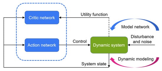
Figure 4. Basic idea of traditional ADP.

Considering the uncertainties and disturbances of the actual system, let $x = {[x_1,x_2]}^{\mathrm{T}} = {[\theta ,\dot{\theta }]}^{\mathrm{T}}$, then SSS (30) is organized as

$$\begin{gathered} \left\{\begin{array}{c}{\dot{x}}_1 = x_2\\ {\dot{x}}_2 = f(x)+g(x)I_{s2}\end{array}\right. \\ y = x_1 \end{gathered}$$

(34)

where $f(x) = -M_{1,s2}^{-1}(\theta ,0)\ddot{\theta }[G_{1,s2}(\theta ,\dot{\theta },0,0)+{\tilde{A}}^{-1}\tilde{B}\dot{\theta }+\psi ]$, $g(x) = M_{1,s2}^{-1}(\theta ,0){\tilde{A}}^{-1}\tilde{C}$, and $f(x)$ and $g(x)$ are both Lipschitz functions.

Assumption 3.

The sum of uncertainties and disturbances $\psi$ in the second slow subsystem has an unknown upper bound ${\psi }^{\ast }$ , which is $‖\psi ‖\le {\psi }^{\ast }$.

Let the desired trajectory and actual trajectory of the subsystem be $x_d$ and $x$, respectively, then the trajectory tracking error is

$$e = x - x_d$$

(35)

We define the performance index as follows

$$J(e(\tau )) = {\displaystyle {\int }_0^{\infty }N}(e(\tau ),I_{s2}(e(\tau )))d\tau$$

(36)

where $N(e(\tau ),I_{s2}(e(\tau ))) = e^{\mathrm{T}}Qe+I_{s2}^{\mathrm{T}}R{I}_{s2}$ is the utility function. There is $N(0,0) = 0$, $N(e,I_{s2}) > 0$ holds for all $e$ and $I_{s2}$, and $Q\in R^{n\times n}$, $R\in R^{m\times m}$ are positive definite matrixes [27].

Let $u_d$ denote the desired control law, then

$$I_{s2}{}_d = g^{+}(x_d)\left({\dot{x}}_d-f(x_d)\right)$$

(37)

Therefore,

$$\dot{e} = \dot{x}-{\dot{x}}_d = f(x)-f(x_d)+g(x)I_{s2}-g(x_d)I_{s2}{}_d$$

(38)

For SSS, the control law $I_{s2}$ includes two parts, desired control $I_{s2}{}_d$ and optimal control $I_{s2}{}_v$, which is

$$I_{s2} = I_{s2}{}_d + I_{s2}{}_v$$

(39)

Therefore,

$$\dot{e} = f_e+[g(x)-g(x_d)]I_{s2}+g(x_d)I_{s2}{}_v$$

(40)

The optimal control $I_{s2}{}_v$ can ensure that the trajectory tracking error of the subsystem converges to the steady state in an optimal manner.

Equation (30) can be rewritten as

$$J(e(\tau )) = {\displaystyle {\int }_0^{\infty }N}(e(\tau ),I_{s2}{}_v(e(\tau )))d\tau$$

(41)

where $N(e,I_{s2}{}_v) = e^{\mathrm{T}}Qe + I_{s2v}^{\mathrm{T}}R{I}_{s2}{}_v$ is the utility function, $N(0,0) = 0$, $N(e,I_{s2}{}_v)>0$ holds for all e and $I_{s2}{}_v$. $I_{s2}{}_v\in \mathsf{\Phi }(\mathsf{\Omega })$ and $\mathsf{\Phi }(\mathsf{\Omega })$ is a set of allowable control sequences.

Definition 1.

For the second slow tracking error subsystem (40), if there exists a set of tolerance controls$I_{s2}(e)\in \mathsf{\Phi }(\mathsf{\Omega })$ that are continuous and satisfy $I_{s2}(e)=0$ when $\mathsf{\forall }e\in \mathsf{\Omega }$, then the subsystem is guaranteed by$I_{s2}(e)$to converge on a compact set with a finite performance index function [34,35].

If the performance index (41) is continuously differentiable, then its infinitesimal form can be expressed as

$$0 = N(e,I_{s2}{}_v)+{(\nabla J(e))}^{\mathrm{T}}(f_e+[g(x)-g(x_d)]I_{s2}+g(x_d)I_{s2}{}_v)$$

(42)

where $J(0)=0$, $N(0,0)=0$, $\nabla J(e)$ is the partial derivatives of with respect to $J(e)$ which is $\nabla J(e) = \frac{\partial J(e)}{\partial e}$.

We define the Hamiltonian function and the optimal performance index as

$$H(e,I_{s2},\nabla J(e)) = N(e,I_{s2}{}_v)+{(\nabla J(e))}^{\mathrm{T}}(f_e+[g(x)-g(x_d)]I_{s2}+g(x_d)I_{s2}{}_v)$$

(43)

$$J^{\ast }(e) = \underset{I_{s2}{}_v}{\min }{\displaystyle {\int }_0^{\infty }N}(e(\tau ),I_{s2}{}_v(e(\tau )))d\tau$$

(44)

Clearly, with $J^{\ast }(e)$ meeting the

$$0 = \underset{I_{s2}{}_v}{\min }H(e,I_{s2}{}_v,\nabla J^{\ast }(e))$$

(45)

where $\nabla J^{\ast }(e) = \frac{\partial J^{\ast }(e)}{\partial e}$.

If $J^{\ast }(e)$ exists and is continuously differentiable, the optimal feedback control law can be solved by a single network evaluation structure strategy iterative algorithm with circular iterations as

$$I_{s2}{{}_v}^{\ast } = -\frac{1}{2}{R}^{-1}{g}^{\mathrm{T}}(x)\nabla J^{\ast }(e)$$

(46)

Combining (42) and (45), we have

$${(\nabla J(e))}^{\mathrm{T}}(f_e+[g(x)-g(x_d)]I_{s2}+g(x_d)I_{s2}{}_v) = -e^{\mathrm{T}}Qe-I_{s2v}^{\mathrm{T}}R{I}_{s2}{}_v$$

(47)

Figure 5 is the single network evaluation structure strategy iteration process. With the control strategy evaluation using Equation (42), based on the evaluation results using Equation (45) to find the optimal feedback control law, in the algorithm, to improve the system regulation effect and performance index function using neural network approximation, there are

$$J(e) = w_{\tau }{}^{\mathrm{T}}{\sigma }_{\tau }(e)+{\epsilon }_{\tau }$$

(48)

where $l$ is the number of neurons in the hidden layer, $w_{\tau }\in R^l$ is the ideal neural network weight, ${\sigma }_{\tau }(e)$ is the neural network activation function and ${\epsilon }_{\tau }$ is the evaluation network approximation error.

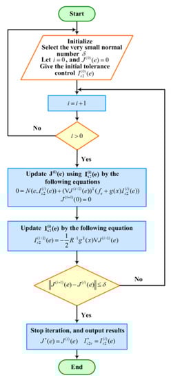
Figure 5. Flowchart of critic-only policy iteration algorithm.

Then, we calculate performance index function gradient $\nabla J(e)$

$$\nabla J(e) = {(\nabla {\sigma }_{\tau }(e))}^{\mathrm{T}}{w}_{\tau } + \nabla {\epsilon }_{\tau }$$

(49)

where $\nabla {\sigma }_{\tau }(e)=\frac{\partial {\sigma }_{\tau }(e)}{\partial e}\in R^{N\times n}$, $\nabla {\epsilon }_{\tau }$ denotes the gradients of ${\sigma }_{\tau }(e)$ and ${\epsilon }_{\tau }$, respectively.

Substituting (49) into (42), we can obtain the Hamiltonian function

$$H(e,I_{s2}{}_v,w_{\tau }) = N(e,I_{s2}{}_v) + (w_{\tau }{}^{\mathrm{T}}\nabla {\sigma }_{\tau }(e))\dot{e} = -\nabla {\epsilon }_{\tau }{}^{\mathrm{T}}\dot{e}\triangleq e_{PH}$$

(50)

where $e_{PH}$ is the residual error of the approximation neural network.

The definitions ${\hat{w}}_{\tau }$ and ${\tilde{w}}_{\tau }$ are, respectively, the estimates and estimation errors of the evaluation neural network weights $w_{\tau }$. Therefore, the output of the evaluation network $\hat{J}(e)$ and its gradient are

$$\begin{gathered} \hat{J}(e) = {\hat{w}}_{\tau }{}^{\mathrm{T}}{\sigma }_{\tau }(e) \\ \nabla \hat{J}(e) = {(\nabla {\sigma }_{\tau }(e))}^{\mathrm{T}}{\hat{w}}_{\tau } \end{gathered}$$

(51)

The approximate Hamiltonian function is

$$H(e,I_{s2}{}_v,{\hat{w}}_{\tau }) = N(e,I_{s2}{}_v)+({\hat{w}}_{\tau }{}^{\mathrm{T}}\nabla {\sigma }_{\tau }(e))\dot{e}\triangleq e_P$$

(52)

The performance criterion that needs to be minimized for the neural network training process [31] is

$$E_P = \frac{1}{2}{e}_P{}^{\mathrm{T}}{e}_P$$

(53)

The weights are then updated using the gradient descent method, with

$${\dot{\hat{w}}}_{\tau } = -{\alpha }_{\tau }{e}_P\eta$$

(54)

where $\eta = \nabla {\sigma }_{\tau }(e)\dot{e}$, ${\alpha }_{\tau }$ is the evaluation network learning rate and ${\alpha }_{\tau } > 0$.

Due to

$${\tilde{w}}_{\tau } = w_{\tau } - {\hat{w}}_{\tau }$$

(55)

we obtain

$$e_P = e_{PH} - w_{\tau }{}^{\mathrm{T}}\nabla {\sigma }_{\tau }(e)\dot{e}$$

(56)

Therefore, the error update rate of the weight estimation is

$${\dot{\tilde{w}}}_{\tau } = -{\dot{\hat{w}}}_{\tau } = {\alpha }_{\tau }(e_{PH}-{\tilde{w}}_{\tau }{}^{\mathrm{T}}\nabla {\sigma }_{\tau }(e)\dot{e})\nabla {\sigma }_{\tau }(e)\dot{e}$$

(57)

The ideal optimal feedback control law and the corresponding iterative control law are

$$\begin{gathered} I_{s2}{}_v = -\frac{1}{2}{R}^{-1}{g}^{\mathrm{T}}(x)({(\nabla {\sigma }_{\tau }(e))}^{\mathrm{T}}{w}_{\tau }+\nabla {\epsilon }_{\tau }) \\ {\hat{I}}_{s2v} = -\frac{1}{2}{R}^{-1}{g}^{\mathrm{T}}(x){(\nabla {\sigma }_{\tau }(e))}^{\mathrm{T}}{\hat{w}}_{\tau } \end{gathered}$$

(58)

Assumption 4.

The desired control law $I_{s2}{}_d$ and $\eta$ both have unknown upper bounds, which are

$$‖I_{s2}{}_d‖\le w_{ud}\hspace{1em}\hspace{1em}‖\eta ‖\le {\eta }_M$$

(59)

Theorem 1.

Under the conditions of Assumptions 3 and 4, if the solution of the neural network-based $\mathrm{HJB}$ equation exists, considering the state space model (30) in SSS and the evaluation network weight update rate (57), if the optimal control law of the system trajectory tracking is chosen as

$$I_{s2} = I_{s2}{}_d+{\hat{I}}_{s2v} = g^{+}(x_d)\left({\dot{x}}_d-f(x_d)\right)-\frac{1}{2}{R}^{-1}{g}^{\mathrm{T}}(x){(\nabla {\sigma }_{\tau }(e))}^{\mathrm{T}}{\hat{w}}_{\tau }$$

(60)

this ensures that both the weight approximation error and the system trajectory tracking error are eventually consistent and bounded.

Proof. 

Considering the Lyapunov theory, we define a positive definite energy function

$$V_1 = \frac{1}{2}{e}^{\mathrm{T}}e+J^{\ast }(e)+\frac{1}{2{\alpha }_{\tau }}{\tilde{w}}_{\tau }^{\mathrm{T}}{\tilde{w}}_{\tau }$$

(61)

Derivative of time, we obtain

$$\begin{array}{cc}\hfill {\dot{V}}_1& =\frac{1}{{\alpha }_{\tau }}{\tilde{w}}_{\tau }^{\mathrm{T}}{\dot{\tilde{w}}}_{\tau }+{(\nabla J^{\ast }(e))}^{\mathrm{T}}\dot{e}+e^{\mathrm{T}}\dot{e}\hfill \\ \hfill & =\frac{1}{{\alpha }_{\tau }}{\tilde{w}}_{\tau }^{\mathrm{T}}{\dot{\tilde{w}}}_{\tau }+{(\nabla J^{\ast }(e))}^{\mathrm{T}}\dot{e}+e^{\mathrm{T}}\left[f_e+[g(x)-g(x_d)]I_{s2}+g(x_d)I_{s2}{}_v\right]\hfill \\ \hfill & =\frac{1}{{\alpha }_{\tau }}{\tilde{w}}_{\tau }^{\mathrm{T}}{\dot{\tilde{w}}}_{\tau }-e^{\mathrm{T}}Qe-I_{s2v}^{\mathrm{T}}R{I}_{s2}{}_v+e^{\mathrm{T}}\left[f_e+[g(x)-g(x_d)]I_{s2}+g(x_d)I_{s2}{}_v\right]\hfill \end{array}$$

(62)

Because $f(x)$ is a $\mathrm{Lipschitz}$ function, there must exist $L_f>0$. When $L_f>0$, it holds $‖f_e‖\le L_f‖e‖$. According to assumption 1, we know that $g(x)$ and $g(x_d)$ are bounded, so we can set

$$‖g(x)‖\le w_g, ‖g(x_d)‖\le w_{gd}$$

(63)

and then

$$‖g(x)-g(x_d)‖\le \Delta w_g$$

(64)

Using the trigonometric inequality, we have

$$\begin{array}{cc}\hfill {\dot{V}}_1& \le L_f{‖e‖}^2+\Delta w_g‖I_{s2}‖‖e‖+w_{gd}‖I_{s2}{}_v‖‖e‖-e^{{\rm T}}Qe-I_{s2v}^{T}R{I}_{s2}{}_v+\frac{1}{{\alpha }_{\tau }}{\tilde{w}}_{\tau }^T{\dot{\tilde{w}}}_{\tau }\hfill \\ \hfill & \le L_f{‖e‖}^2+\Delta w_g‖I_{s2}{}_d+I_{s2}{}_v‖‖e‖+w_{gd}‖I_{s2}{}_v‖‖e‖-e^{{\rm T}}Qe-I_{s2v}^{T}R{I}_{s2}{}_v+{\tilde{w}}_{\tau }^T(e_{PH}-{\tilde{w}}_{\tau }^T\eta )\eta \hfill \\ \hfill & \le L_f{‖e‖}^2+\Delta w_g‖I_{s2}{}_d‖‖e‖+\frac{1}{2}\Delta w_g{}^2{‖I_{s2}{}_v‖}^2+\frac{1}{2}{‖e‖}^2+{\tilde{w}}_{\tau }^T{e}_{PH}\eta \hfill \\ \hfill & +\frac{1}{2}{w}_{gd}{}^2{‖e‖}^2-{‖{\tilde{w}}_{\tau }^T\eta ‖}^2+\frac{1}{2}{‖I_{s2}{}_v‖}^2-{\lambda }_{\min }(R){‖I_{s2}{}_v‖}^2-{\lambda }_{\min }(Q){‖e‖}^2\hfill \\ \hfill & \le -\left[\left({\lambda }_{\min }(Q)-L_f-\frac{1}{2}{w}_{gd}{}^2-\frac{1}{2}\right)‖e‖-\Delta w_g‖I_{s2}{}_d‖\right]‖e‖\hfill \\ \hfill & -\left({\lambda }_{\min }(R)-\frac{1}{2}\Delta w_g{}^2-\frac{1}{2}\right){‖I_{s2}{}_v‖}^2+\frac{1}{2}{e}_{PH}^2-\frac{1}{2}{‖{\tilde{w}}_{\tau }^{\mathrm{T}}\eta ‖}^2\hfill \\ \hfill & \le -\left[\left({\lambda }_{\min }(Q)-L_f-\frac{1}{2}{w}_{gd}{}^2-\frac{1}{2}\right)‖e‖-\Delta w_g{w}_{ud}\right]‖e‖\hfill \\ \hfill & -\left({\lambda }_{\min }(R)-\frac{1}{2}\Delta w_g{}^2-\frac{1}{2}\right){‖I_{s2}{}_v‖}^2+\frac{1}{2}{e}_{PH}^2-\frac{1}{2}{‖{\tilde{w}}_{\tau }^{\mathrm{T}}\eta ‖}^2\hfill \end{array}$$

(65)

Clearly, in the collections

$$\begin{gathered} {\mathsf{\Omega }}_1 = \left\{{\tilde{w}}_{\tau }:‖{\tilde{w}}_{\tau }‖\le \frac{e_{PH}}{{\eta }_M}\right\} \\ {\mathsf{\Omega }}_2 = \left\{e:‖e‖\le \frac{\Delta w_g{w}_{ud}}{{\lambda }_{\min }(Q)-L_f-\frac{1}{2}{w}_{gd}{}^2-\frac{1}{2}}\right\} \end{gathered}$$

(66)

in addition to them, and they must satisfy the conditions

$$\begin{gathered} {\lambda }_{\min }(Q) \ge L_f+\frac{1}{2}{w}_{gd}{}^2+\frac{1}{2} \\ {\lambda }_{\min }(R) \ge \frac{1}{2}\Delta w_g{}^2+\frac{1}{2} \end{gathered}$$

(67)

Then, there is

$${\dot{V}}_1 \le 0$$

(68)

Thus, considering the Lyapunov stability theory, both the joint angle tracking error in SSS and the neural network weight approximation error are eventually consistent and bounded.

This completes the proof. □

4.2. Robust Optimal Vibration Control

Aiming at designing the optimal control law using the quadratic form, the model of SFS is rewritten as

$${\dot{X}}_k = A_k{X}_k + B_k{I}_{f2}$$

(69)

where $X_k=\left[\begin{array}{c}{y}_{f2}\\ \frac{d{y}_{f2}}{d{\sigma }_2}\end{array}\right]$, $A_k=\left[\begin{array}{cc}0& E\\ -D_{4,s2}\left(\theta ,{\epsilon }_{2}y\right)\tilde{K}& 0\end{array}\right]$, $B_k=\left[\begin{array}{c}0\\ D_{3,s2}\left(\theta ,{\epsilon }_{2}y\right){\tilde{A}}^{-1}\tilde{C}\end{array}\right]$.

The control purpose is that the appropriate control law is proposed to adjust the system state to zero, that is, suppress elastic vibrations in SFS. It is easy to verify that it is completely controllable, and the optimal control method can be used, since SFS is a linear system.

The quadratic performance index function is selected as follows:

$$J_k = \frac{1}{2}{\displaystyle {\int }_0^{\infty }[X_k^{\mathrm{T}}Q{X}_k+I_{f2}^{\mathrm{T}}R{I}_{f2}]dt}$$

(70)

The algebraic Riccati equation can be written as

$$A_k^{\mathrm{T}}P+P{A}_k-P{B}_k{R}^{-1}{B}_k^{\mathrm{T}}P+Q=0$$

(71)

Then, the optimal feedback control law is

$$I_{f2}=-K_f{X}_k=-R^{-1}{B}_k^{\mathrm{T}}P{X}_k$$

(72)

A robust optimal control law with great dynamic performance is given below to ensure the stability of the system while there are uncertainties in SFS. Therefore, we obtain the dynamic equation with uncertainties

$${\dot{X}}_k = (A_{k0}+\Delta A_k)X_k+B_k{I}_{f2}$$

(73)

Theorem 2.

For the second fast subsystem with parameter uncertainty, if the uncertainty satisfies

$${‖\Delta A_k‖}_2<\frac{{\lambda }_{\min }}{2\rho (P)}$$

where ${\lambda }_{\min }$ is the minimum eigenvalue of $Q+P{B}_k{R}^{-1}{B}_k^{\mathrm{T}}P$ and $\rho (P)$ is the spectral radius of $P$, and $I_{f2}$ is elected optimal control law (72), the closed loop asymptotic stability of SFS can be guaranteed.

Proof. 

Considering the Lyapunov theory, define the second positive definite energy function

$$V_2 = X_k^{\mathrm{T}}P{X}_k$$

(74)

Substituting (69), (72) and (73) into the time derivative of Equation (74), we obtain

$$\begin{array}{cc}\hfill {\dot{V}}_2& ={\dot{X}}_k^{\mathrm{T}}P{X}_k+X_k^{\mathrm{T}}P{\dot{X}}_k\hfill \\ \hfill & =X_k^{\mathrm{T}}(A_{k0}^{\mathrm{T}}P+P{A}_{k0}-2P{B}_k{R}^{-1}{B}_k^{\mathrm{T}}P)X_k+2X_k^{\mathrm{T}}P\Delta A_k{\dot{X}}_k\hfill \\ \hfill & =-X_k^{\mathrm{T}}(Q+P{B}_k{R}^{-1}{B}_k^{\mathrm{T}}P)X_k+2X_k^{\mathrm{T}}P\Delta A_k{\dot{X}}_k\hfill \end{array}$$

(75)

Because both $P$ and $Q+P{B}_k{R}^{-1}{B}_k^{\mathrm{T}}P$ are symmetric matrices, we have

$$\begin{gathered} 2X_k^{\mathrm{T}}P\Delta A{\dot{X}}_k<2\rho (P)\cdot {‖\Delta A_k‖}_2\cdot {‖X_k‖}_2^2 \\ \frac{X_k^{\mathrm{T}}(Q+P{B}_k{R}^{-1}{B}_k^{\mathrm{T}}P)X_k}{X_k^{\mathrm{T}}{X}_k}>{\lambda }_{\min } \end{gathered}$$

(76)

Substituting inequality (76) into Equation (75), we have

$${\dot{V}}_2 < [2\rho (P)\cdot {‖\Delta A_k‖}_2-{\lambda }_{\min }]{‖X_k‖}_2^2$$

(77)

When the inequality ${‖\Delta A_k‖}_2 < \frac{{\lambda }_{\min }}{2\rho (P)}$ holds, ${\dot{V}}_2$ will be less than 0. Hence, the second fast closed-loop subsystem is stable.

This completes the proof. □

4.3. Adaptive Sliding Mode Servo Control

In the actual work of the hydraulic servo control system, there are some uncertain factors such as the perturbation of the elastic modulus of hydraulic oil, hydraulic oil leakage and friction of moving parts. They will directly affect the stability and dynamic characteristics of the hydraulic servo control subsystem. Therefore, the dynamics of FFS with uncertainties will be from Equation (21) to

$$\frac{d{\tau }_{f1}}{d{\sigma }_1}+{\tilde{A}}_0{\tau }_{f1}+F = {\tilde{C}}_0{I}_{f1}$$

(78)

where $F = \Delta \tilde{A}{\tau }_{f1}-\Delta \tilde{C}{I}_{f1}$ is the overall uncertainty, and it is bounded.

If $\hat{F}$ is the estimated value of $F$, define the estimated error

$$\tilde{F} = F-\hat{F}$$

(79)

We define the tracking error vector

$$\begin{gathered} e_f = {\tau }_{f1d} - {\tau }_{f1} \\ {\dot{e}}_f = {\dot{\tau }}_{f1d}-{\dot{\tau }}_{f1} \end{gathered}$$

(80)

then select a sliding surface

$$s_f = e_f$$

(81)

Theorem 3.

Considering the hydraulic servo FFS, the ASMC is presented as

$$I_{f1} = {\tilde{C}}_0^{-1}[\frac{d{\tau }_{f1}}{d{\sigma }_1}+{\tilde{A}}_0{\tau }_{f1}+\hat{F}+\xi \mathrm{sgn}(s_f)]$$

(82)

$$\dot{\hat{F}} = {\Lambda }^{\mathrm{T}}{s}_f$$

(83)

Then, the closed-loop FFS is uniformly ultimately stable.

Proof. 

Considering the Lyapunov theory, we define the third positive definite energy function

$$V_3 = \frac{1}{2}{s}_f^{\mathrm{T}}{s}_f + \frac{1}{2}{\tilde{F}}^{\mathrm{T}}{\Lambda }^{\mathrm{T}}\tilde{F}$$

(84)

Differentiate (84) with respect to time, and we can have

$$\begin{array}{ll}\hfill {\dot{V}}_3& =s_f^{\mathrm{T}}{\dot{s}}_f+{\dot{\tilde{F}}}^{\mathrm{T}}{\Lambda }^{-1}\tilde{F}\hfill \\ \hfill =& s_f^{\mathrm{T}}(\frac{d{\tau }_{f1}}{d{\sigma }_1}+{\tilde{A}}_0{\tau }_{f1}+F-\tilde{C}{I}_{f1})-{\dot{\hat{F}}}^{\mathrm{T}}{\Lambda }^{-1}\tilde{F}\hfill \\ \hfill =& s_f^{\mathrm{T}}(F-\hat{F}-\xi \mathrm{sgn}(s_f))-s_f^{\mathrm{T}}\Lambda {\Lambda }^{-1}\tilde{F}\hfill \\ \hfill & =-s_f^{\mathrm{T}}\xi \mathrm{sgn}(s_f)\hfill \\ \hfill & \le 0\hfill \end{array}$$

(85)

From (85), $V_3(s_f(t))\le V_3(s_f(0))$, so $s_f(t)$ is bounded. Considering the Lyapunov function as $V_4=-s_f^{\mathrm{T}}k{s}_f$, the integration of $V_4$ can be obtained as ${\displaystyle {\int }_0^{\infty }{V}_4}(\tau )d\tau \le V_3(s_f(0))-V_3(s_f(\infty ))\le \infty$. Therefore, it is concluded that error can asymptotically converge to zero as $t\to \infty$ based on Barbalat Lemma.

This completes the proof. □

4.4. Composite Control

According to the theoretical analysis above, the control law for the HDFRMS by (16) can be expressed as (60), (72), (82) and (83). Additionally, Figure 6 is the whole block diagram for the manipulator control closed-loop system.

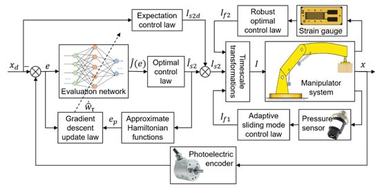
Figure 6. Block diagram of HDFRMS with controllers.

In Figure 6, the desired angles and angle velocities $x_d$ after trajectory planning are provided as input to the manipulator system. Meanwhile, three control outputs $I_{s2}$, $I_{f2}$ and $I_{f1}$ can be individually calculated using information measured by the sensors such as photoelectric encoders, pressure sensors and strain gauges. However, these control outputs are then summed after timescale transformation. At last, the closed-loop HDFRMS with control schemes can be realized.

Theorem 4.

The stabilities of SSS (30), SFS (33) and FFS (21) are guaranteed under adaptive dynamic programming trajectory control law (60), robust optimal vibration control law (72) and adaptive sliding mode servo control law (82) and (83), based on SPT. Therefore, the closed-loop stability of the whole manipulator system (16) can be guaranteed under the composite controller.

5. Simulations

In this section, some simulation results (implemented in MATLAB) are analyzed to indicate the effectiveness and robustness of the singular perturbation decoupling method and proposed composite control laws in previous parts. All the tests are conducted on the HDFRMS, whose dynamics is given in (16) with these structure parameters (see Table 3).

Table 3. HDFRMS structure parameters.

Notation	Value	Unit	Notation	Value	Unit	Notation	Value	Unit
$L_1$	1.8	m	${\rho }_1$	20	kgm−1	$C_{di}$	0.85	----
$L_2$	2.5	m	${\rho }_2$	40	kgm−1	$C_d$	0.8	----
$L_3$	6	m	${\rho }_3$	40	kgm−1	$C_{tm1}$	$7\times {10}^{-13}$	m5/N·s
$L_{11}$	1	m	$A_1$	0.015	m2	$C_{tmi}$	$5\times {10}^{-13}$	m5/N·s
$L_{21}$	0.2	m	$A_2$	0.02	m2	$P_s$	$7\times {10}^6$	Pa
$L_{22}$	1	m	$EI$	${10}^7$	Nm2	$w_i$	$0.08$	m
$L_{31}$	0.2	m	$V_t$	0.002	m3	$w$	0.04	m
$r_1$	0.2	m	$K_{ci}$	$6\times {10}^{-13}$	m3/pa·s	${\beta }_e$	$7\times {10}^8$	Nm−2
$r_2$	0.4	m	$K_c$	$4\times {10}^{-13}$	m3/pa·s	$D$	0.2	m2
$m_2$	5	kg	$K_{ii}$	$10$	cm/A	$L$	1.2	m
$m_3$	8	kg	$K_i$	$8$	cm/A	$\rho$	$870$	kgm−3

In ADP trajectory control, the back propagation (BP) neural network, the critic neural network, is selected as 6-8-1 with 6 input neurons, 8 hidden neurons and 1 output neuron (see Figure 7). Additionally, its activation function, learning rate and initial weight values are selected as sigmoid function, ${\alpha }_{\tau } = 0.02$, and ${\hat{w}}_{\tau 0} = {[\begin{array}{cccccccc}1.4& 1.7& 0.6& 1.3& 0.4& 1.9& 0.8& 0.9\end{array}]}^{\mathrm{T}}$, respectively.

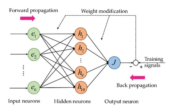
Figure 7. The structure of BP neural network.

In addition, the parameters of robust optimal vibration control and adaptive sliding mode servo control can be given as $Q = diag(\begin{array}{cccc}55& 65& 40& 60\end{array})$, $R = diag(\begin{array}{ccc}15& 10& 24\end{array})$, $\xi = diag(\begin{array}{ccc}27& 36& 28\end{array})$, $\mathsf{\Lambda } = diag(\begin{array}{ccc}60& 90& 85\end{array})$.

The initial positions of the manipulator joints are selected as ${\theta }_{d0} = {[1 0.1 0.2]}^{\mathrm{T}}$, and their desired trajectories as chosen as ${\theta }_d = {[0.75\cos 2t-0.1+0.8\sin 1.5t0.5\cos t]}^{\mathrm{T}}$.

The sampled time instant is 0.1 ms. Time taken is 10 s. The simulations are illustrated in Figure 8, Figure 9, Figure 10, Figure 11, Figure 12 and Figure 13.

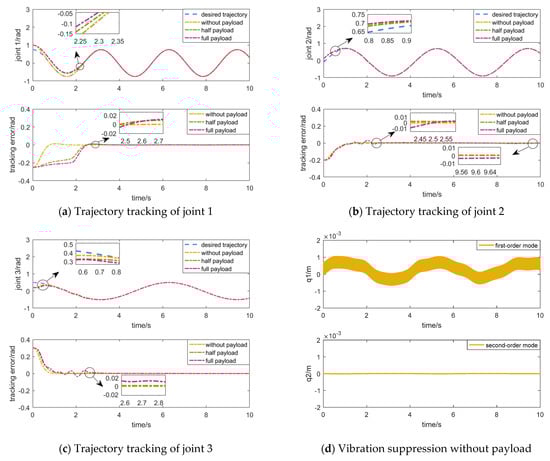
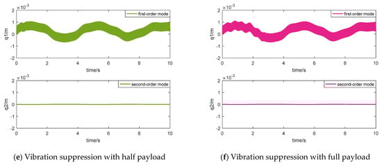
Figure 8. Tracking performances and vibration suppression of the manipulator without uncertainties.

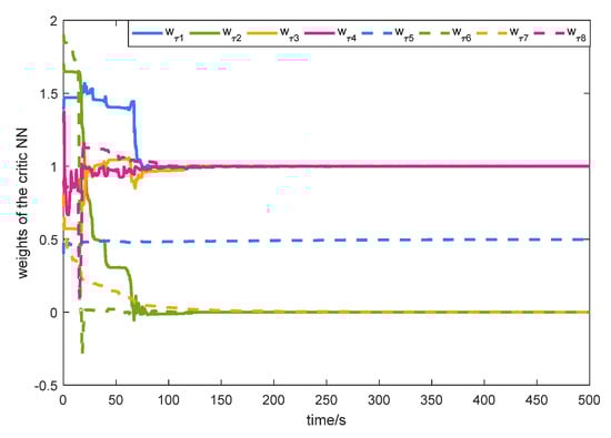
Figure 9. Weights of critic neural network.

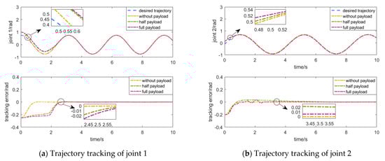
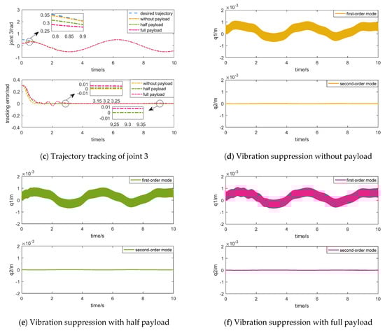
Figure 10. Tracking performances and vibration suppression of the manipulator with uncertainties.

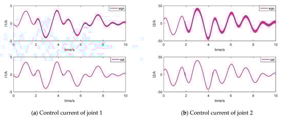
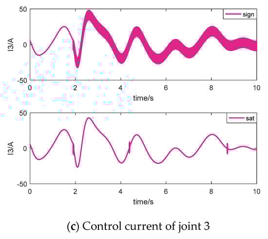
Figure 11. Control current comparisons with full payload and uncertainties.

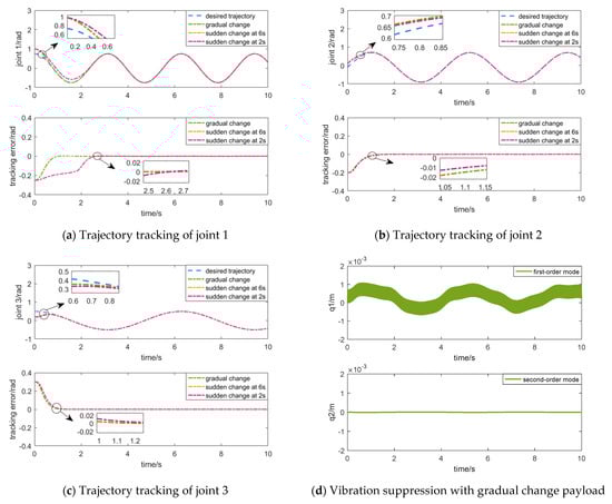
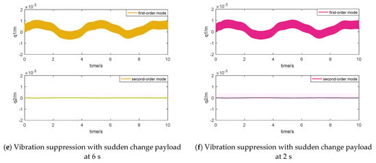
Figure 12. Tracking performances and vibration suppression of the manipulator with uncertainties in different conditions with varying payload.

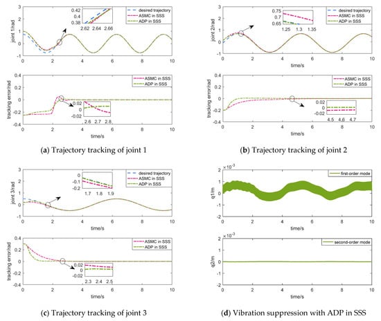
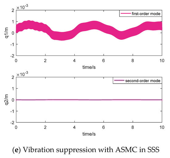
Figure 13. Comparison with the ASMC in SSS.

5.1. Reference-Tracking Performance in System without Uncertainties

When there is no uncertainty in HDFRMS, the tracking performances of joints (see Figure 8a–c) and vibration suppression of the flexible link 3 (see Figure 8d–f) are tested. Both simulations and numerical results use the same control parameters under several different working conditions, including the end-effector without payload ($M = 0 \mathrm{kg}$), with half payload ($M = 300 \mathrm{kg}$) and with full payload ($M = 600 \mathrm{kg}$).

Figure 8a–c indicates that all joint angles can quickly track to the prospective trajectories in 3 s or less. In particular, the trajectory tracking speed of joint 1 is faster than other joints because of the rotary joint, which is insensitive to vibrations. Figure 8d–f shows that both first-order mode and second-order mode can be controlled effectively, even if the vibration suppression needs to spend 3 s handling full payload. However, only forced vibration caused by a large range of joint motion exists in system. In addition, Figure 9 illustrates that the weights of the critic neural network converge to ${[\begin{array}{cccccccc}0.994& 0.003& 1.001& 1.013& 0.499& -0.007& 0.002& 1.007\end{array}]}^{\mathrm{T}}$.

5.2. Reference-Tracking Performance in System with Uncertainties

To verify the robustness of HDFRMS closed-loop system, as shown in Figure 10 and Figure 11, the total uncertainties $\psi$ in SSS and the uncertainties $F$ in FFS are chosen as $\psi = {\left[\begin{array}{ccc}0.001\sin 1.5t+0.0004rand(1)& 0.0005\cos t+0.0005rand(1)& 0.0005\sin 0.5t+0.0005rand(1)\end{array}\right]}^{\mathrm{T}}$ and $F = {\left[\begin{array}{ccc}0.001\cos 5t+0.001rand(1)& 0.001\sin 3.5t+0.001rand(1)& 0.001\sin 4t+0.001rand(1)\end{array}\right]}^{\mathrm{T}}$, respectively. Then, both the sine and cosine function are used to express parameter uncertainties in the manipulator system, and the random function represents external disturbances and noises.

Figure 10 shows the tracking performances of joints and vibration suppression of the third flexible arm in HDFRMS with uncertainties. Compared to the previous cases, the tracking time of joint angle 2, nearly 3.5 s, is the longest response time of the system according to Figure 10a–c. Furthermore, the tracking error fluctuation of joint angle 3 is less than 0.01 rad between 9.2 s and 9.5 s, because of the combined effects of system uncertainties, accumulated errors, full payload and motion coupling. However, the largest error fluctuating ranges can satisfy the requirements of steady state. Figure 10d–f shows that the vibration is also so small and can be suppressed quickly.

The chattering comparisons of control currents with full payload and uncertainties are shown in Figure 11. Clearly, the chattering can be weakened by the saturation function whose boundary layer is 0.01 instead of the sign function.

5.3. Reference-Tracking Performance in System with Varying Payloads and Uncertainties

To test if the composite controller is more adaptive in the condition of varying payloads, three working conditions are considered. The first working condition is that the payload mass is gradual changed from 600 kg to 0 kg, starting from 0 s to 6 s. The other working conditions are that the payload mass is suddenly changed from 600 kg to 200 kg at 6 s and 2 s.

Figure 12 shows the tracking performances and vibration suppression of the manipulator with uncertainties in different conditions with varying payloads. Table 4 is the composite controller performance comparisons with uncertainties, where three evaluation criteria for the trajectory tracking errors are adopted: the root mean squared error (RMSE), integral squared error (ISE), and integral absolute error (IAE) [36].

Table 4. Controller performance comparisons with uncertainties.

Error Accuracy	Joint	Without Payload	Half Payload	Full Payload	Gradual Change	Sudden Change (2 s)	Sudden Change (6 s)
RMSE	1	1.29	1.16	0.97	1.03	1.12	1.12
$({10}^{-3}$)	2	1.76	1.63	1.34	1.39	1.61	1.59
	3	2.24	2.07	1.79	1.92	2.03	2.01
ISE	1	5.43	5.18	4.91	4.99	5.05	5.05
$({10}^{-4}$)	2	5.88	5.50	5.37	5.43	5.50	5.50
	3	6.96	6.74	6.44	6.62	6.69	6.67
IAE	1	3.15	2.85	2.74	2.59	2.77	2.77
$({10}^{-3}$)	2	3.87	3.16	3.39	3.24	3.52	3.51
	3	4.02	3.66	3.93	3.69	3.80	3.80

Figure 12a–c indicates that the tracking error converges faster than the sudden change of mass, when the payload mass changes gradually. The settling time is about 1 s. In addition, the convergence rate of tracking error is almost the same whether the sudden time is 2 s or 6 s. Their error curves nearly coincide (see Figure 12a–c) and their RMSE, ISE and IAE are almost the same (see Table 4). Therefore, the sudden change in mass does not affect the tracking performance of manipulator system, whether in the transition process or in the steady state.

5.4. The Comparison with the ASMC in SSS

We chose an ASMC that can deal with uncertain systems to compare with ADP in SSS. The ASMC can be designed as

$$\begin{array}{c}\hfill I_{s2} = {\tilde{C}}^{-1}\tilde{A}(M_{1,s2}(\theta ,0){\ddot{\theta }}_r+{\tilde{A}}^{-1}\tilde{B}{\dot{\theta }}_r+G_{1,s2}(\theta ,\dot{\theta },0,0)+\hat{\psi }+\epsilon sa\mathrm{T}(s_s))\hfill \\ \hfill {\dot{\theta }}_r={\dot{\theta }}_d+\lambda ({\theta }_d-\theta )\hfill \\ \hfill \dot{\hat{\psi }}={{\rm Y}}^{\mathrm{T}}{s}_s\hfill \end{array}$$

(86)

where $\epsilon =diag(40,35,20)$, $\lambda =diag(25,25,45)$ and ${\rm Y}=diag(240,185,200)$. The closed-loop stability proof with ASMC is similar to this paper [37].

The payload mass is selected as 450 kg. The uncertainties and other controller parameters remain unchanged, consistent with previous simulations.

The simulation results can be seen in Figure 13, indicating that the transient response of the ADP in SSS is significantly faster than that of the ASMC. The ASMC has few superiorities for trajectory tracking, and the longer settling time will inevitably lead to larger average errors. In particular, the settling time of joint angle 2 is more than 4 s (see Figure 13b). Moreover, the vibration suppression of the first-order mode becomes worse in the transition process when ASMC is used in SSS and other controllers remain the same as before.

In summary, the composite controller proposed in this paper can adequately represent the manipulator trajectory tracking performances under six different cases because controller parameters always remain constant. Additionally, the control has greater robustness with system uncertainties, no matter how the payload mass is changed. Compared with the ASMC with the same robustness, the settling time of ADP is shorter.

6. Conclusions

This paper discusses the dynamics modeling and trajectory tracking control of HDFRMS in practical engineering applications. The dynamics of the manipulator system, which are modeled as AMM and the Lagrange principle, are decomposed into second slow, second fast and first fast subsystem describing the rigid motion, flexible vibration and servo-hydraulic-driven control, based on SPT. The control laws of all subsystems with independent state variables can be designed respectively. Additionally, the adaptive dynamic programming trajectory tracking control with critic-only policy iteration algorithm, robust optimal vibration control and adaptive sliding mode servo control are established by the Lyapunov stability theory, while the total uncertainty boundary in HDFRMS is unknown. Finally, numerical simulations successfully demonstrate that the composite controller is not only effective but also robust.

Although it was not the focus of this paper, we believe that the cross-scale decoupling method can be extended to rigid–flexible, macro–micro, and electro–hydraulic complex multi-body dynamics systems. Moreover, the selection of perturbation parameters and their influences on the system should be further studied. Additionally, we will also discuss how to improve robustness for further research based on ADP, when frictions of hydraulic cylinder exist in the manipulator servo actual system.

References

- Yang, H.J.; Liu, J.K. Distributed piezoelectric vibration control for a flexible-link manipulator based on an observer in the form of partial differential equations. J. Sound Vib. 2016, 363, 77–96. [Google Scholar] [CrossRef]
- Lu, E.; Li, W.; Yang, X.F.; Wang, Y.Q.; Liu, Y.F. Dynamic modeling and analysis of a rotating piezoelectric smart beam. Int. J. Struct. Stab. Dyn. 2018, 18, 1850003. [Google Scholar] [CrossRef]
- Liu, Y.F.; Li, W.; Yang, X.F. Coupled dynamic model and vibration responses characteristic of a motor-driven flexible manipulator system. Mech. Sci. 2015, 6, 235–244. [Google Scholar] [CrossRef]
- Xu, B.; Yuan, Y. Two performance enhanced control of flexible-link manipulator with system uncertainty and disturbances. Sci. China Inf. Sci. 2017, 60, 050202. [Google Scholar] [CrossRef]
- Ju, J.Y.; Li, W.; Wang, Y.Q. Vibration observation for a translational flexible-link manipulator based on improved Luenberger observer. J. Vibroeng. 2016, 18, 238–249. [Google Scholar]
- Su, Y.; Mueller, P.C.; Zheng, C. Global asymptotic saturated PID control for robot manipulators. IEEE Trans. Control Syst. Technol. 2010, 18, 1280–1288. [Google Scholar] [CrossRef]
- Zamora-Gomez, G.; Zavala-Río, A.; Lpez-Araujo, D.; Santibáñez, V. Further results on the global continuous control for finite-time and exponential stabilisation of constrained-input mechanical systems: Desired conservative force compensation and experiments. IET Control Theory Appl. 2019, 13, 159–170. [Google Scholar] [CrossRef]
- Riad, A.; Meddahi, H. A fast adaptive artificial neural network controller for flexible link manipulators. Int. J. Adv. Comput. Sci. Appl. 2016, 7, 298–308. [Google Scholar] [CrossRef]
- Li, F.; Zhang, Z.; Wu, Y.; Chen, Y.; Liu, K.; Yao, J. Improved fuzzy sliding mode control in flexible manipulator actuated by PMAs. Robotica 2022, 40, 2683–2696. [Google Scholar] [CrossRef]
- Dog, M.; Istefanopulos, Y. Optimal nonlinear controller design for flexible robot manipulators with adaptive internal model. IET Control Theory Appl. 2007, 1, 770–778. [Google Scholar]
- Bastos, G. A non-inherent parametric estimation for dynamical equivalence of flexible manipulators. Optim. Control Appl. Methods 2022, 43, 825–841. [Google Scholar] [CrossRef]
- Mehrez, M.W.; El-Badawy, A.A. Effect of the joint inertia on selection of under-actuated control algorithm for flexible-link manipulators. Mech. Mach. Theory 2010, 45, 967–980. [Google Scholar] [CrossRef]
- Lu, E.; Li, W.; Yang, X.; Liu, Y.F. Modelling and composite control of single flexible manipulators with piezoelectric actuators. Shock Vib. 2016, 7, 2689178. [Google Scholar] [CrossRef]
- Xu, B. Composite learning control of flexible-link manipulator using NN and DOB. IEEE Trans. Syst. 2018, 48, 1979–1985. [Google Scholar] [CrossRef]
- Siciliano, B.; Book, W.J. A singular perturbation approach to control of lightweight flexible manipulators. Int. J. Robot. Res. 1988, 7, 79–90. [Google Scholar] [CrossRef]
- Cheng, X.; Zhang, Y.J.; Liu, H.S.; Wollherr, D.; Buss, M. Adaptive neural backstepping control for flexible-joint robot manipulator with bounded torque inputs. Neurocomputing 2021, 458, 70–86. [Google Scholar] [CrossRef]
- Xu, B.; Shi, Z.K.; Yang, C.G. Composite fuzzy control of a class of uncertain nonlinear systems with disturbance observer. Nonlinear Dyn. 2015, 80, 341–351. [Google Scholar] [CrossRef]
- Cheng, X.; Liu, H.S.; Zeng, Z.; Lu, W.K. Robust fuzzy sliding mode control and vibration suppression of free-floating flexible-link and flexible-joints space manipulator with external interference and uncertain parameter. J. Dyn. Syst. Meas. Control Trans. Asme 2022, 144, 1004–1015. [Google Scholar]
- Xie, L.M.; Yu, X.Y.; Chen, L. Saturated Output Feedback Control for Robot Manipulators With Joints of Arbitrary Flexibility. Robotica 2022, 40, 997–1019. [Google Scholar] [CrossRef]
- Dindorf, R.; Wos, P. A Case Study of a Hydraulic Servo Drive Flexibly Connected to a Boom Manipulator Excited by the Cyclic Impact Force Generated by a Hydraulic Rock Breaker. IEEE Access 2022, 10, 7734–7752. [Google Scholar] [CrossRef]
- Franco, E.; Garriga-Casanovas, A.; Tang, J.; Baena, F.R.; Astolfi, A. Adaptive energy shaping control of a class of nonlinear soft continuum manipulators. IEEE/ASME Trans. Mechatron. 2022, 27, 280–291. [Google Scholar]
- Zeng, H.; Sepehri, N. On tracking control of cooperative hydraulic manipulators. Int. J. Control 2007, 80, 454–469. [Google Scholar] [CrossRef]
- Zhang, X.; Shi, G. Dual extended state observer-based adaptive dynamic surface control for a hydraulic manipulator with actuator dynamics. Mech. Mach. Theory 2022, 169, 104647. [Google Scholar]
- Li, S.; Zhu, K.; Chen, L.; Yan, Y.; Guo, Q. Variable Structure Disturbance Observer Based Dynamic Surface Control of Electrohydraulic Systems with Parametric Uncertainty. Energies 2022, 15, 1671. [Google Scholar]
- Irani, A.N.; Talebi, H.A. Tip tracking control of a rigid-flexible manipulator based on deflection estimation using neural network. In Proceedings of the ISSNIP Biosignals and Biorobotics Conference 2011, Vitoria, Brazil, 6–8 January 2011; pp. 1–6. [Google Scholar]
- Merritt, H.E. Hydraulic Control Systems; Wiley: New York, NY, USA, 1967. [Google Scholar]
- Zhao, J.; Wang, T.; Pedrycz, W.; Wang, W. Granular prediction and dynamic scheduling based on adaptive dynamic programming for the blast furnace gas system. IEEE Trans. Cybern. 2019, 51, 2201–2214. [Google Scholar] [CrossRef]
- Wang, X.; Quan, Z.; Zhang, J. Optimal 3-dimension trajectory-tracking guidance for reusable launch vehicle based on back-stepping adaptive dynamic programming. Neural Comput. Appl. 2022, 35, 5319–5334. [Google Scholar]
- Ren, X.; Li, H. Adaptive dynamic programming-based feature tracking control of visual servoing manipulators with unknown dynamics. Complex Intell. Syst. 2022, 8, 255–269. [Google Scholar] [CrossRef]
- Hu, C.; Zhao, L.; Qu, G. Event-Triggered Model Predictive Adaptive Dynamic Programming for Road Intersection Path Planning of Unmanned Ground Vehicle. IEEE Trans. Veh. Technol. 2021, 70, 11228–11243. [Google Scholar] [CrossRef]
- Xia, H.; Zhao, B.; Li, Y. Optimal tracking control for reconfigurable manipulators based on critic-only policy iteration algorithm. In Proceedings of the 2017 36th Chinese Control Conference (CCC), Dalian, China, 26–28 July 2017; pp. 2616–2621. [Google Scholar]
- Liu, D.; Wang, D.; Li, H. Decentralized stabilization for a class of continuous-time nonlinear interconnected systems using online learning optimal control approach. IEEE Trans. Neural Netw. Learn. Syst. 2014, 25, 411–428. [Google Scholar]
- Zhao, B.; Liu, D.; Li, Y. Online fault compensation control based on policy iteration algorithm for a class of affine nonlinear systems with actuator failures. IET Control Theory Appl. 2016, 10, 1816–1823. [Google Scholar] [CrossRef]
- Zhang, H.; Cui, L.; Zhang, X.; Luo, Y. Data-driven robust approximate optimal tracking control for unknown general nonlinear systems using adaptive dynamic programming method. IEEE Trans. Neural Netw. 2011, 22, 2226–2236. [Google Scholar] [CrossRef]
- Abu-Khalaf, M.; Lewis, F.L. Nearly optimal control laws for nonlinear systems with saturating actuators using a neural network HJB approach. Automatica 2005, 4, 779–791. [Google Scholar] [CrossRef]
- Kuo, C.W.; Tsai, C.C.; Lee, C.T. Intelligent leader-following consensus formation control using recurrent neural networks for small-size unmanned helicopters. IEEE Trans. Syst. Man Cybern. Syst. 2019, 51, 1288–1301. [Google Scholar] [CrossRef]
- Tang, Z.G.; Shan, X.H.; Li, S.T. Dynamic Modeling and Extension Adaptive Sliding Mode Control of Onboard Craning Manipulator. IFAC-PapersOnLine 2020, 53, 530–535. [Google Scholar]
Disclaimer/Publisher’s Note: The statements, opinions and data contained in all publications are solely those of the individual author(s) and contributor(s) and not of MDPI and/or the editor(s). MDPI and/or the editor(s) disclaim responsibility for any injury to people or property resulting from any ideas, methods, instructions or products referred to in the content. |
© 2023 by the authors. Licensee MDPI, Basel, Switzerland. This article is an open access article distributed under the terms and conditions of the Creative Commons Attribution (CC BY) license (https://creativecommons.org/licenses/by/4.0/).