Creation of Signals Database for the Development of Speed Estimation in an Axle Counter System

Abstract

The article presents the process of creation of a signals database for the development of a train speed-estimation method for an axle counter system. In the article the authors present the need for information about the train speed on the railway lines and the possible applications for which the information about the train speed may be used, as well as address the concerns related with the evaluation of the information in axle counter systems. The main goal of the paper is to present the creation process of an axle counter signals database and how to emulate the real signals using the laboratory-obtained ones. A database that has been created for a specific wheel detector is available on request. It contains a variety of signals that are necessary for the development and tests of wheel detector algorithms, in particular the estimation of train speed. Signals were generated for the most commonly used rail profile in Europe and the wheels that are defined in the technical specification of interoperability. Furthermore, the signals were transformed to emulate various speeds, the possible accelerations and to include the disturbance observed in the field.

1. Introduction

Train detection systems play an important role in the rail signaling systems. They provide information about train positions in the railway infrastructure, which is crucial for managing the traffic in a safe way. Apart from the basic information about the track section unoccupancy, the system may provide other valuable information such as, e.g., speed of the moving trains. Highly accurate and safe information about the actual speed of a train is very important for control over a train movement. Starting from the train driver who needs to know the current speed of the vehicle, through the automatic train protection systems (ATP), which monitor the permitted speed and if it is exceeded activate braking, up to a fully automatic train operation (ATO), which not only slows down the train if the speed is too high, but allows to operate the train in a fully automatic, driverless mode. For such purposes, the speed is measured by tachometers [1,2] that are parts of the train equipment. In [3] the authors discussed different methods of speed estimation based on the encoders installed on the axles of vehicles. The method based on optical technology [4], Global Positioning System (GPS) [5] or Eddy-Current sensors [6] can also be used, but they all involve vehicle equipment. Information about the speed is then available for the driver, the onboard systems and, in the case of ERTMS (European Rail Traffic Management System), also for the RBC (Radio Block Centre) thanks to the GMS-R communication (GMS for Railways) [7].

The information about the train speed may be also very useful for other systems that use axle counters but have no access to the information provided by vehicle equipment. The systems which may use the information about the train speed are for example: a level crossing—operator notification system (class A level crossing system), an automatic level crossing system and an information system for passengers waiting at the platforms. The data about the train speed may be also used as diagnostic information, especially for monitoring the condition of the tracks [8,9] and for the purpose of performing the End-of-Train detection function.

The standardization of rail traffic control systems in Europe includes the train speed as a one piece of information to be provided by axle counter systems. The initiative is led by the EULYNX consortium, established by the leading European Infrastructure Managers (inter alia: DB Netz, Pro Rail, SNCF, Infrabel, Network Rail and many others). The current available standard for the interface between the Train Detection Systems (TDS), including axle counters and the interlocking systems, the main interfaced system for TDS, i.e., the SCI-TDS Specification doc. SCI-TDS Eu.Doc.44 v3.3 (Set 4) specifies the message with information about the train speed and a wheel diameter. Today, there are no safety requirements imposed by EULYNX for providing such information (Basic Safety according to CENELEC EN 50129 [10]), however it may be expected that it will change in the future, if such information is used for purposes other than just for diagnostic ones.

In the case of the first two applications (Level Crossing systems), the speed of the train may be used to delay the barrier closing. In [11], the authors present an issue of barriers closed for a long time being a bottleneck for the traffic on the level crossing and propose a solution based on the continuous vehicle and infrastructure communication. A more dangerous situation happens when the people waiting next to the closed level crossing try to circumvent the barriers and cross the tracks. Lack of a train for a long time (and even 2 min may be a long time for waiting people) results in irrational human behavior, leading to dangerous situations. According to Polish Railway Infrastructure Manager (PKP PLK S.A.) ca. 98% of the accidents on the level crossings is caused by car drivers and pedestrians trying to cross the tracks when the barriers are closed (hurry, impatience, rashness) (5521 Level Crossing Systems installed on PKP PLK network in 2020, 12,457 in total) [12].

The maximum speed of the trains for the track/road crossings is V_MAX = 160 km/h (Polish Railway Infrastructure Manager, according to [13]). The distance at which the triggering sensor is installed depends on the maximum allowed speed on the line and may reach up to d = 3 km (Figure 1).

The distance d and the current train speed have a significant influence on travel time, e.g., the time of 67 s by a train moving at the speed of 160 km/h (V_MAX) or for 9 min by a train moving at 20 km/h. Knowing the train speed it is possible to avoid closing the barrier too early, thereby preventing an unpredictable and dangerous behaviors of the waiting people. It increases the safety on the level crossings. Such predictions and functionality are also required by some Customers and known as a “Constant Warning Time”. The time between the barrier closing and the moment when a train appears at the level crossing shall be constant, independent of the train speed. In [14] authors present the solution based on the two inductive sensors, while the information of the train speed evaluated by a single detector is more desirable due to reduction of equipment costs.

The information about the speed may be also useful for the axle counter system itself. The following functions may be supported by the information about the speed of the train: validation of the wheel counting, switching the filter parameters or controlling the decision (counting) algorithm parameters.

The ability to evaluate information about the train speed in compliance with a specific Safety Integrity Level, i.e., SIL-4 acc to EN 50128 is crucial for enabling the use of the information on train speed for the purpose of ensuring supervision by the signaling systems in the applications referred to herein. At the time of writing the paper, there was no such solution available on the market. There are axle counters which provide information about the speed but it is done according to the basic safety integrity level (SIL-0) or the speed is estimated by means of more than one detector, as it has been already mentioned. The potential dependence of the wheel detector signal on the wheel and rail profiles, and their condition, as well as the position of a wheel in relation to the rail (based on the authors’ experience) poses the main challenge for evaluating the speed by a wheel detector. The speed estimation with the assumed accuracy and safety in such a situation is a challenge and this is probably the reason why such solutions are still not available. Verification of this hypothesis and further preparation of a robust speed-estimation algorithm for a wheel detector requires creating of a database of signals to be used during the development and tests of the relevant solution. Such a database must include representative population of signals which may appear during the operation of a wheel detector and based on which the information about the speed is evaluated. Field measurements, however valuable, can only be used as a final confirmation that the prepared algorithm provides information about the speed of a train with required accuracy.

A streamlined methodology for creating a signals database is presented in Figure 2 below.

The first step is to determine the operational conditions of the application for which such a database is intended to be used. Depending on the principle of wheel detector operation the samples of wheels must be prepared to gather the wheel signatures. Once the wheel signatures are collected, they can be then used for generating signals including other factors such as, e.g., different speeds, acceleration or disturbances which may appear in the field. The validation step is based on the comparison of the generated signals with examples of the real ones that have been registered in the field. This is valuable. However, registration of signals in the field is affected by high uncertainty related to the conditions of measurements, like an unknown real wheel diameter, a wheel position or sometimes even a real train speed. The measurement campaigns with fully available rolling stock are very costly and thus very rare.

Nevertheless, when the database is ready, it shall be a basis for development and laboratory tests. The potentially developed algorithm will then be subject to validation tests in the field which may sometimes even last for a few months.

The engineers who work on the wheel detection technology are the main contributors to the research. The process of creating the signals database is universal and can be applied by various manufacturers, however the database itself shall be created individually for each type of a wheel detector as it is specific and depends on wheel detection technology.

The created database is also intended for the scientists who may be interested in contributing to the development of algorithms that are to be used in the axle counter systems.

2. Creation of Signals Database Measurement Conditions

Conventional axle counter systems operate based on the inductive sensors (detectors) mounted on the rails (such devices are located all over the world in many countries). The passage of a wheel changes the signal, which then is subject to analysis and wheel counting. Depending on the design of the sensor the signal may be intensified (Figure 3) or be suppressed while the wheel appears over it.

In order to detect the direction of train movement, sensors usually comprise two channels which in the end produce signals in a form of voltages u₁ and u₂ (Figure 3). During the wheel passage the signals are changing in time, but in fact they are changing with the movement of the wheel along the sensor. Such signals are then named “wheel signatures” as their shape mainly depends on the wheel profile.

The shape of the signal depends on the following factors:

• the rail profile and condition (the level of wear & tear);
• the wheel profile and condition;
• the lateral position of a wheel in relation to the rail and wheel detector head (sensor).

The input data are gathered in the laboratory conditions on the specially dedicated test stand. During the measurements in the field, even if the known train is moving with the known speed, the lateral position of a wheel is accidental and not repeatable. It is also not feasible in the field to measure all the possible wheel profiles moving on the rails in different conditions.

The rails, wheels and their position on the rail generates many combinations of measurement configurations. The number of combinations may be decreased. Typically, it is possible in relation to the rail profile and its condition for which the detector is approved to be used (e.g., 60E1 with lateral wear (L) up to 10 mm; vertical wear (V) up to 20 mm and mixed V/L = 10/5 mm). The number of types of wheels may also be reduced, however, it is rather possible in the mass transit applications (metro, trams) due to a limited volume of types of vehicles or into a certain extent in the railways (e.g., TSI compliant rolling stock). Wheel types may also be limited by means of defining the minimum dimensions of a flange, a wheel diameter and a rim width. However these features are not so easy to be monitored, like rail types, which do not change.

2.1. Rails

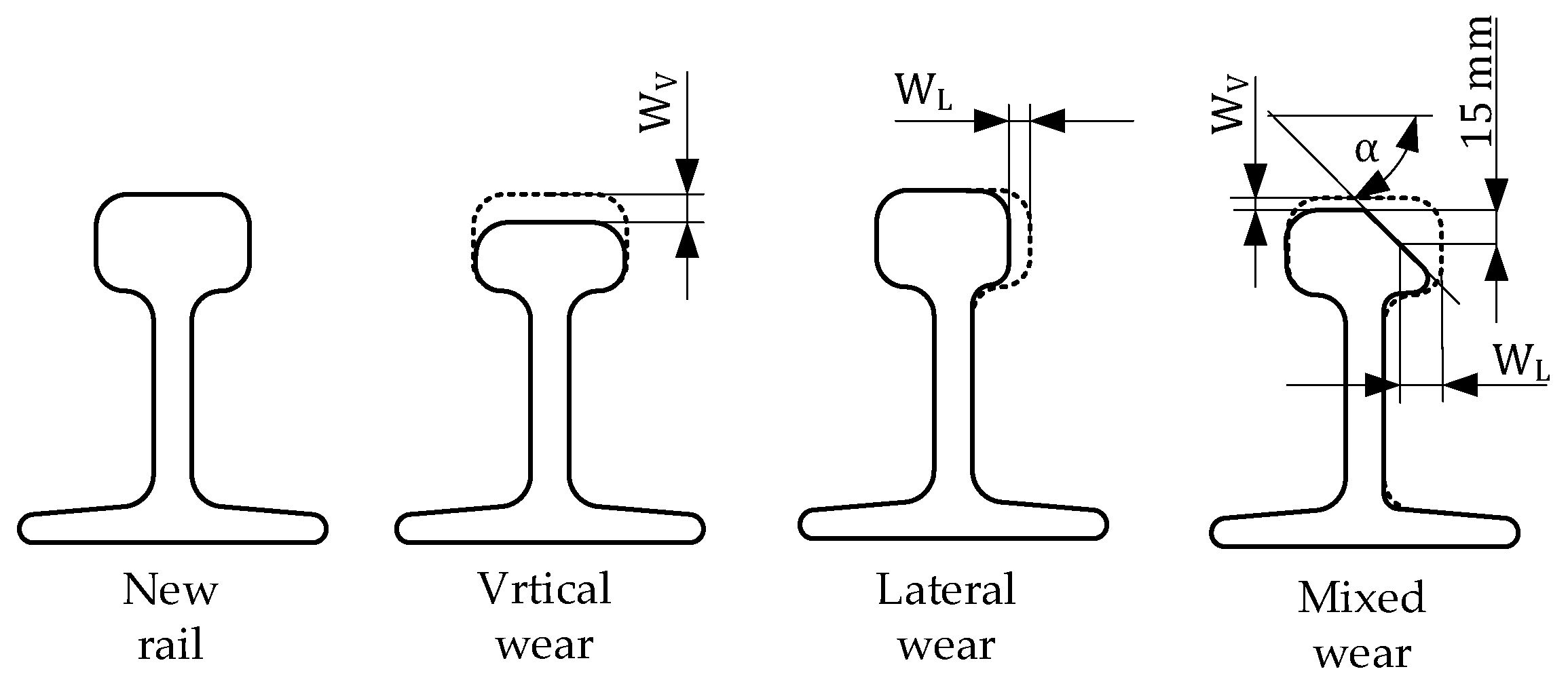
The wheel signatures are gathered for each type of a rail (R) for which system must provide reliable information about train speed. Nowadays 60E1 (UIC 60) is the most popular rail profile not only in Europe. However, for example: 115 RE (according to. AREMA standard in America) or AS68 (Australian Standard) can be found on other continents. In the East, P60, P65 or P68 (Russian Standard) are used. The degree of wear and tear, if not specified, is an individual decision of the axle counter provider. In the case of 60E1 it can reach up to 20 mm of vertical wear (W_V) and 22 mm of lateral (W_L; from class 0 to class 5 of tracks, according to [15], Table 1, Appendix 14). It is also recommended to acquire signals for mixed vertical and lateral wear, as it is more natural. According to [15] in such a case, the maximum, allowed vertical wear shall be decreased by half of the real lateral one. The value of angle α is equal to 55°, 60° or 65°, depending on the class of track (Figure 4). Maximum wear and tear of the rail shall be defined by the Infrastructure Manager and depends on the category of tracks (main lines, industrial, urban, stabling yard).

Example of parameters of 60E1 for the main lines (class 0, according to [15], Table 1 Appendix 14) is as follows:

• a new rail: W_V < 5 mm, W_L < 5 mm (assumption);
• a maximum vertical wear: W_V = 12 mm;
• a maximum lateral wear: W_L = 14 mm;
• a mixed wear: W_V = 5, W_L = 14 mm.

The combination of rail wear may be reduced in the situation when the position of a sensor (detector head) is adjusted during the periodical maintenance and its relation to the wheel is ensured, independently of the condition of the rail. If the impact of the rail dimensions is negligible (e.g., a detector is sensitive only to the flange of a wheel), the measurement may be limited to the single type of a rail.

2.2. Wheel Profile

The spectrum of wheel profiles (W) on the railways is very high. The number of configurations may be reduced based on a standard whose use is confirmed by the relevant Infrastructure Manager. Technical Specification for Interoperability (TSI) for Railways (TSI) in Europe is one of them and defines the parameters of the rolling stock for interoperable lines. The parameters of the wheels and wheel sets are defined in doc.: ERA/ERTMS/033281 [16]. The document defines, among others, dimensions of wheels such as a diameter, a rim width, a flange height and a flange thickness (Figure 5) for different track gauges irrespective of the rail profiles.

The flange height (S_h) and thickness (S_d) (see Figure 5) are described in [16] as a function of wheel diameter D. The gauge of 1435 mm, which covers also the wheels for gauges 1524 mm and 1668 mm is treated as the reference for Railways in Europe. Such wide tracks as 1520 mm, very popular in the East, and 1600 mm gauge (that is used for instance in Ireland), require preparing additional samples of wheels.

The set of wheel samples $\mathbf{W} \in \{ \mathrm{k}2, \mathrm{k}4, \mathrm{k}5, \mathrm{k}6, \mathrm{k}8, \mathrm{k}10, \mathrm{k}11, \mathrm{k}13, \mathrm{k}15, \mathrm{k}16\}$ presented in the

Table 1. Wheel profiles.

Wheel Profile W	Diameter D [mm]	Flange Height Sh [mm]	Flange Thickness Sd [mm]
k2	330	32	27.5
k4	600	32	27.5
k5	600	36	33
k6 *	632	29	14.8
k8 *	640	25	23.9
k10	760	32	27.5
k11	760	36	33
k13	820	36	33
k15	840	36	33
k16	820	26	27.5

* tram wheels, based on one of Alstom’s application requirements (nominal—k8 and a worn one—k6). Tram wheels are added additionally for comparison purposes (heavy railway vs. mass transit).

covers the profiles specified in [6]. Minimum dimensions of a wheel flange are most critical for operation of the inductive sensor and thus are used to specify the samples for signal database creation.

2.3. Wheel Position on the Rail

For the preparation of the test data, the signals are acquired also for different lateral positions of the wheel. The TSI says only that the wheel flange may be located at some distance from the rail head, but it does not define it in millimeters. The various positions result from the tolerances for the dimensions of rails, tracks (gauge), wheels and wheelbases. The maximum lateral distance of a flange p (Figure 5), equal to 60 mm is defined in [17], which specifies the parameters of axle counter systems for interoperability in Europe.

where $\mathbf{p} \in \left\{{ \mathrm{p}}_0{, \mathrm{p}}_1{, \mathrm{p}}_2\right\}$:

• p₀, nominal position (0 mm); the flange of the wheel is as close as possible to the head of the rail;
• p₁, moved laterally; the flange is moved aside from the rail head up to 60 mm (as required by [17]);
• p₂, maximum; the flange is moved aside from the rail head up to the maximum feasible position (for the safety margin, see

  Table 2. The lateral position of wheel.

  Wheel Profile W	Position p0 [mm]	Position p1 [mm]	Position p2 [mm]
  k2	0	60	83
  k4	0	60	85
  k5	0	60	82
  k6	0	60	70
  k8	0	60	70
  k10	0	60	83
  k11	0	60	83
  k13	0	60	81
  k15	0	60	88
  k16	0	60	83

  ):

2.4. Rail and Wheel Material

Wheel signatures may be gathered on the real or specially prepared samples of rails and wheels. If extra samples are used, it is important to make them from the material with the same magnetic and electric characteristics like of the real ones. Typically, rails used for tests are the real ones and sometimes artificially worn, however in the case of using samples it is important to prepare them from ferromagnetic and electrically conducting material. Samples of wheels are typically specially prepared. It allows to cover a wide range of dimensions, as well as is more ergonomic (lower weight) and economic (lower cost). For the majority of the inductive sensors, it is sufficient to use a small part of the rim with a flange instead of a full-size wheel (the part of the wheel detected by the sensor). The TSI [16] says that they must be made of the ferromagnetic and electrically conducting materials.

3. Acquired Data

3.1. Signal Acquisition

A wheel signature is a change of voltage signal u₁ and u₂ (sensor head signal) as a function of the position of the wheel on the rail in relation to the sensor (s). In fact, this signature does not depend only on the wheel profile (W), including its wear & tear but on its lateral position (p_i) and may also depend on a rail profile and its condition (R).

The wheel signature may be obtained automatically in the following way:

(a)

by means of recording the signals u₁ and u₂ for the wheel moving on the rail as a function of the position s. This method gives directly the “wheel signatures” as a function U = f(s, p, W, R). This method is independent on the speed of the moving wheel, however it requires additional information about the position s (Figure 3).

(b)

by means of recording the signals u₁ and u₂ for the wheel moving at constant speed along the rail as a function of time. This method gives the wheel signatures as a function U = f(t, p, W, R), that can be recalculated for the position of wheel (u = f(s)) as the speed is known and is constant. It does not require any additional signals to be measured. The center of a head may be used as a reference point where both signals u₁ and u₂ cross (Figure 3).

The first method (a) gives a wheel signature directly. The number of samples for the wheel signature, while recorded with the density of one sample per millimeter, would be around 300 (for sensor sensitivity area equal to 30 cm). In the case of a wheel moving at 1 km/h and 10 kSps of the wheel detector sampling rate, 10,800 samples are acquired. It means that, to obtain the same resolution between each sample recorded using method (a), 36 new samples must be added.

The second method (b), used during measurements does not require any additional signal except u₁ and u₂. To avoid the need for interpolation, the signals are recorded for wheel moving at a constant speed of 1 km/h and sampled exactly with the same frequency, like a wheel detector works (f_i).

If the speed is different, then it is standardized to 1 km/h by a resampling method or by means of adjusting the sampling rate for gathering the signal (f_m) to the real speed of a moving wheel according to the formula:

$${\mathrm{f}}_{\mathrm{m}}\left[\mathrm{Hz}\right]{=\mathrm{f}}_{\mathrm{i}}\left[\mathrm{Hz}\right]·\frac{\mathrm{v}\left[\mathrm{km}/\mathrm{h}\right]}{1\mathrm{km}/\mathrm{h}}$$

(1)

where:

• ${\mathrm{f}}_{\mathrm{m}}$—sampling rate for signal recording,
• ${\mathrm{F}}_{\mathrm{i}}$—operating sampling rate of detector,
• $\mathrm{v}$—speed of a moving wheel.

Both methods provide the buffer of samples reflecting the signals recorded with the speed of 1 km/h and may be transformed to a different speed by means of a decimation method (down sampling).

3.2. Obtained Wheel Signatures

Signals were gathered at the test stand (Figure 6) which enabled moving a wheel at a constant speed of v = 0.028 m/s (0.1 km/h) with its precise lateral and vertical position (Section 3.1, method “b”).

The head of a wheel detector (sensor) was installed on the rail and connected to the trackside electronic unit, which provided signal u₁ and u₂ for registration. Sampling frequency according to Formula (1) was equal to f_m = 1000 sps (for sampling rate of detector f_i = 10 ksps).

The created database contains records (passage in both directions) of u₁ and u₂ signals for the assumed configurations:

• a wheel profile $W \in \{ \mathrm{k}2, \mathrm{k}4, \mathrm{k}5, \mathrm{k}6, \mathrm{k}8, \mathrm{k}10, \mathrm{k}11, \mathrm{k}13, \mathrm{k}15, \mathrm{k}16\}$ (see Table 1)

Wheel samples were made of S235 steel. The rim and flange dimensions were compliant with ERA/ERTMS/033281 [16], except for tram wheels;

• lateral position on a rail $\mathbf{p} \in \left\{ {\mathrm{p}}_0{, \mathrm{p}}_1{, \mathrm{p}}_2\right\}$ (see Table 2);
• rail type R: 60E1 (UIC60), 1 m of a real, new rail.

Records are made in the text files (csv) in two columns, containing voltages of u₁ and u₂ in mV, comma-separated, fixed point format, five digits per sample:

Example:

00640,00550,

00670,00530,

…

sample1 (n = 1): u1(n) = 640 mV, u2(n) = 550 mV

sample2 (n = 2): u1(n) = 670 mV, u2(n) = 530 mV

Each file (record) contains 34,999 samples (n = 1, ..., 34,999) and for sampling period T_i = 100 µs (f_i = 10 ksps) represents the passage of a wheel at a constant speed of 1 km/h.

The wheel signatures referred to above are treated as reference data.

4. Test Signals Transformation—Extending the Database for Testing Purposes

To reflect the real, operational conditions, the acquired signals, i.e., wheel signatures are further modified to simulate a different speed, acceleration or disturbances.

Document [16] defines some wheel and wheelsets parameters as a function of the maximum train speed. Although the speed is not presented as a requirement, it is an information about the train speed at which axle counters/wheel detectors (and thus developed algorithms) shall work properly to cover all the possible applications in Europe. Document [17] is more precise and specifies that axle counters shall work at the speed from 0 to 350 km/h, when, on the one hand, in the case of level crossing applications, the maximum speed is lower i.e., 160 km/h and on the other hand in the case of new high speed lines it is higher (e.g., 400 km/h, high speed lines in the UK).

None of the documents concerning axle counter systems addresses the maximum acceleration or de-acceleration during train braking, at which axle counters shall work. The value which can be found in the list of parameters for electrical traction units defines the maximum acceleration on the level of 1.3 m/s² for the initial phase of movement (i.e., 0–50 km/h; 0.8 m/s² above) and −1.4 m/s² during the emergency braking [18]. The value from −2 m/s² to 2 m/s² is therefore considered for the purpose of signals database creation.

4.1. Different Speed Emulation—Scaling in Time

When there is a buffer of signals, recorded for the certain speed, i.e., 1 km/h (called wheel signatures), it can be easily transformed to match higher speed using a decimation method (down sampling, Figure 7). Through taking every Δn sample from the buffer, we will obtain the shape of a signal for the speed equal to Δn∙1 km/h.

In the case of decreasing the speed, it can be achieved by means of interpolation (up-sampling) method. The same sample from the original signal appears Δn times in the new buffer, and it decreases the speed by Δn times. Such a mechanism includes zero-hold interpolation for filing the gaps between the following n samples and can be used for small Δn.

For higher level of up-sampling, it is recommended to fill the gaps with (Δn—1) zero values and use an output filter (Figure 8). For this method each u[n] sample shall be multiplied by Δn to obtain the proper output signal.

The pass band of output filter (f_p), presented in Figure 8 shall be limited to the maximum frequency existing in the signal, which is about 300 Hz (taking into consideration the wheel signature) for the speed of 450 km/h (400 km/h is currently required for axle counters for highspeed lines in Europe). An example of increasing the speed is shown in Figure 9 and reducing the speed in Figure 10.

4.2. Acceleration/De-Acceleration Simulation

The rolling stock, especially the light one (locomotive only; metro/tram rolling stock) may change the speed rapidly. Such a situation shall be recognized by the algorithm and included in the calculation, or such a signal shall be excluded from the speed estimation completely.

When the signal u(n) is registered for a certain speed (e.g., ${\mathrm{v}}_0$ = 1 km/h) in the buffer, the asymmetry being the result of acceleration or de-acceleration (braking) may be generated based on the following formula:

$${\mathrm{u}}_{\mathrm{a}}\left[\mathrm{m}\right]=\mathrm{u}\left[\mathrm{n}\right]$$

(2)

where:

$$\mathrm{n}=\frac{{2\mathrm{v}}_0{\mathrm{m}+\mathrm{am}}^2{\mathrm{T}}_{\mathrm{i}}}{2\mathrm{v}}$$

(3)

$$\mathrm{m}=1\dots \mathrm{M} \cap \mathrm{n}, \mathrm{m} \in \mathrm{N}, \mathrm{n} \le { \mathrm{n}}_{\max }$$

(4)

• $\mathrm{u}\left[\mathrm{n}\right]$—nth sample of signal u(n), registered for v = v₀ = const.,
• ${\mathrm{u}}_{\mathrm{a}}\left[\mathrm{m}\right]$—mth sample of signal u(m), accelerated or deaccelerated,
• ${\mathrm{T}}_{\mathrm{i}}$—sampling period of $u\left[n\right]$ signal in [s],
• ${\mathrm{v}}_0$—initial speed in [m/s], for the presented method always equal to $\mathrm{v}$,
• $\mathrm{v}$—speed for which u(n) has been recorded (or recalculated)—in this case 0.28 m/s (1 km/h),
• $\mathrm{a}$—acceleration ($\mathrm{a} > 0$)/deacceleration ($\mathrm{a} < 0$) in [m/s²].

The idea of transformation in order to simulate acceleration and deacceleration is presented in Figure 11. The signal u(n) is the one registered originally for constant speed (or is the result of resampling). Accelerated or deaccelerated signal is calculated based on Formulas (2) and (3). The acceleration is based on non-linear compressing of the original signal when the de-acceleration is a kind of stretching signal with zero-hold approximation (n is rounded down).

For further processing different situations of speed changes presented in Figure 12 are considered, including linear and step change of the speed. The decimation or interpolation method is used for the step change of speed.

Linear change of the speed, with constant acceleration a is more practical, whereas theoretical step change provides more significant and visible effects and thereby is useful for testing of robustness of an algorithm.

During de-acceleration, the speed is decreased and after time t_gr reaches zero. It generates additional conditions for signal transformation:

$${\mathrm{v}}_0+\mathrm{at} \ge 0, \mathrm{a} < 0 ⟹ \mathrm{t} \le -\frac{{\mathrm{v}}_0}{\mathrm{a}}$$

(5)

$${\mathrm{for} \mathrm{t}=\mathrm{mT}}_{\mathrm{i}} ⟹ \mathrm{m} \le -\frac{{\mathrm{v}}_0}{{\mathrm{aT}}_{\mathrm{i}}}$$

(6)

$${\mathrm{for} \mathrm{t}}_{\mathrm{gr}}{=\mathrm{m}}_{\mathrm{gr}}{\mathrm{T}}_{\mathrm{i} }⟹{ \mathrm{m}}_{\mathrm{gr}}=\frac{-{\mathrm{v}}_0}{{\mathrm{aT}}_{\mathrm{i}}}$$

(7)

The above condition means, that:

$$f{\mathrm{or} \mathrm{m} > \mathrm{m}}_{\mathrm{gr} }⟹ \mathrm{u}\left[\mathrm{m}\right]=\mathrm{u}\left[{\mathrm{m}}_{\mathrm{gr}}\right]$$

(8)

Example of transformation of signals (Figure 9A) is presented in Figure 13 and Figure 14.

In the signal presented in Figure 13A, the wheel stops after t_gr = 3 s and it does not change anymore. Other parameters: v = v₀ = 0.28 m/s, a = 0.5 m/s² for acceleration and a = −0.2 m/s² for deacceleration, t₀ = 1.7 s.

In the created signal presented in Figure 14, the speed has changed 3 times: v1 = 3∙v0 for acceleration and v1 = (1/3)∙v0 for de-acceleration; t₀ = 1.7 s.

4.3. Disturbance Simulation

The real signal contains also noise and distortions coming from the electric motors or railway infrastructure [19]. The basic approach to introducing this kind of disturbance is to add a noise and pulse d(n) to the wheel signature u(n). Such a model does not include the limitation of the bandwidth introduced by the hardware design of the wheel detector, but it is the worst-case scenario for testing. To include the impact of analog path of the detector, an additional low-pass filter for disturbances is used (Figure 15A). The solution presented in Figure 15B includes also the impact of this filter on the wheel signature signal for higher speed.

The filter used shall reflect the frequency characteristic of the analog part of wheel detector.

In the case of the wheel detector concerned, it is a low-pass, Butterworth IIR digital filter, with the characteristic shown in Figure 16 and the following parameters:

• cut-off frequency (F_cutoff): 300 Hz,
• stop band edge (F_stop): 600 Hz
• pass band attenuation (A_pass): 3 dB
• stop band attenuation (A_stop): 60 dB
• filter order: 10

The pass band attenuation (A_pass) of 3 dB for the cut-off frequency equals to 300 Hz (0.3 kHz) as well as stop band attenuation (A_stop) of 60 dB for frequency of 600 Hz (0.6 kHz) are presented as a dashed line in Figure 16.

Filter coefficients, 5x Second Order Section (SOS) are presented in

Table 3. Filter coefficients for sections 1–3.

Filter Coeff.	Section 1	Section 2	Section 3
b(0)	0.00879706726769769083	0.00834036423798943660	0.00798761629247967363
b(1)	0.01759413453539538166	0.01668072847597887320	0.01597523258495934725
b(2)	0.00879706726769769083	0.00834036423798943660	0.00798761629247967363
a(1)	−1.90723559039974510654	−1.80822074306518110198	−1.73174372911906848671
a(2)	0.94242385947053586293	0.84158220001713901492	0.76369419428898721591

and

Table 4. Filter coefficients for section 4 and 5.

Filter Coeff.	Section 4	Section 5
b(0)	0.00774948665490224689	0.00762990106715701923
b(1)	0.01549897330980449378	0.01525980213431403845
b(2)	0.00774948665490224689	0.00762990106715701923
a(1)	−1.68011637353610687740	−1.65418979117563558212
a(2)	0.71111432015571585108	0.68470939544426367984

.

For single SOS (y—output of section, x—input of section):

$$\mathrm{y}\left[\mathrm{n}\right]=\mathrm{b}\left(0\right)\mathrm{x}\left[\mathrm{n}\right]+\mathrm{b}\left(1\right)\mathrm{x}\left[\mathrm{n}-1\right]+\mathrm{b}\left(2\right)\mathrm{x}\left[\mathrm{n}-2\right] - \mathrm{a}\left(1\right)\mathrm{y}\left[\mathrm{n}-1\right] - \mathrm{a}\left(2\right)\mathrm{y}\left[\mathrm{n}-2\right]$$

(9)

The filter is a digital equivalent of the hardware filter used in the design of the subjected wheel detector, 10th order, low-pass filter (LTC1569-6). Impact of unilinear phase of the filter used during the signal preparation as it is applied for the randomly generated disturbances is considered negligible.

4.3.1. Adding Noise

The basic solution is to use the white noise as a source of continuous disturbance added to the signal. The standard deviation σ of the noise shall be scaled to the value observed for subjected detector operating in the field.

$${\mathrm{u}1}_{\mathrm{d}}\left(\mathrm{n}\right)=\mathrm{u}1\left(\mathrm{n}\right)+\mathrm{k}·\mathrm{d}1\left(\mathrm{n}\right)$$

(10)

$${\mathrm{u}2}_{\mathrm{d}}\left(\mathrm{n}\right)=\mathrm{u}2\left(\mathrm{n}\right)+\mathrm{k}·\mathrm{d}2\left(\mathrm{n}\right)$$

(11)

where:

$$\mathrm{d}1, \mathrm{d}2 - \mathrm{white} \mathrm{noise}, \mathsf{\sigma }=1$$

(12)

Factor k shall be selected in such way that the standard deviation of the disturbance is on the same level as observed in the wheel detector operates in the field. The white noise presented in Figure 17 (k = 0.05) is an equivalent of the continuous disturbance overlapping the signal, for which the standard deviation σ is equal to 50 mV [9].

4.3.2. Impulse Disturbance

An impulse disturbance has an impact on the wheel detector signal. Such a phenomenon can be caused by the discharge on the catenary during rising or falling of the pantograph, driving with power through the neutral sections (change of the feeding system) or other commutations in the traction system.

Impulse disturbance may be simulated as a Kronecker Delta signal, defined as:

$$\mathsf{\delta }\left(\mathrm{i}\right)=\{\begin{array}{l}1, \mathrm{for} \mathrm{i}=0\\ 0, \mathrm{for} \mathrm{i} \ne 0\end{array}$$

(13)

The disturbance can be added to the wheel signature as presented on the Figure 14, scaled by “k” and shifted by “m” samples to simulate different moment in time when the disturbance affects the signal (Equations (14) and (15)).

$${\mathrm{u}1}_{\mathrm{d}}\left(\mathrm{n}\right)=\mathrm{u}1\left(\mathrm{n}\right)+\mathrm{k}·\mathsf{\delta }\left(\mathrm{n} - \mathrm{m}\right)$$

(14)

$${\mathrm{u}2}_{\mathrm{d}}\left(\mathrm{n}\right)=\mathrm{u}2\left(\mathrm{n}\right)+\mathrm{k}·\mathsf{\delta }\left(\mathrm{n} - \mathrm{m}\right)$$

(15)

Both signals u1 and u2 are affected in the same moment, which is typical for such types of disturbance (effect of commutations). To obtain effects on the detector signal that are observed in the field, Kronecker delta should be scaled by an extremely high factor (e.g., k = 1000) to achieve high enough energy. Such a signal is not transferred by the detector so a more natural approach is to replace it by the pulse with a lower amplitude (i.e., the maximum one which may be transferred by the wheel detector) and lasting longer.

Pulse disturbances appear rarely so it is sufficient to add a single pulse per a whole wheel signature at various points in time (different “m”), as it is presented in Figure 18.

The delay “m” may be generated randomly. Pulses shall be generated in the same, as well as in the opposite phase in the case of signals u1 and u2 (as observed in the field, Figure 19).

5. Results

As a result of transformation of wheel signatures, described in Section 4 of the paper, a database of signals containing over 13,000 test files has been prepared. The files contain records of signals u1 and u2 for the wheel detector concerned for different speeds, accelerations and disturbances in respect of the following parameters:

• Speed: ${\mathrm{v}}_0 \in \{ 1 \mathrm{km}/\mathrm{h}, 10 \mathrm{km}/\mathrm{h}, 50 \mathrm{km}/\mathrm{h}, 100 \mathrm{km}/\mathrm{h}, 150 \mathrm{km}/\mathrm{h}, 200 \mathrm{km}/\mathrm{h}\}$ and for each speed as well (folder name):
• AccelerationX_Y: X = 1: a₁ = 0.5 m/s², X = 2: a₂ = 1.0 m/s², X = 3: a₃ = 2.0 m/s² for each v₀;
• BrakingX_Y (de-acceleration): X = 1: a₁ = −0.05 m/s², X = 2: a₂ = −0.10 m/s², X = 3: a₃ = −0.20 m/s² for v₀ = 1 km/h and X = 1: a₁ = −0.50 m/s², X = 2: a₂ = −1.00 m/s², X = 3: a₃ = −2.00 m/s² for v₀ = 10 km/h ÷ 200 km/h.

In respect to acceleration and de-acceleration the time t₀ (according to Figure 12) was equal to the value presented in

Table 5. Delay t₀.

	Y = 0	Y = 1
V0 [km/h]	t01 [s]	t02 [s]
1	1.0	1.65
10	0.1	0.165
50	0.02	0.033
100	0.01	0.0165
150	0.0066	0.011
200	0.005	0.00825

:

• WhiteNoise: σ = 50 mV (k = 0.05 V);
• PulseX_Y: X = 1: symmetric positive (Figure 19A), X = 2: symmetric negative, X = 3 and X = 4: asymmetric (Figure 19B) added to the signal with six different delays td, depending on the speed (Table 6):

Table 6. Delay t_d of the pulse disturbance added to the signal.

	Y = 0	Y = 1	Y = 2	Y = 3	Y = 4	Y = 5
V0 [km/h]	td1 [s]	td2 [s]	td3 [s]	td4 [s]	td5 [s]	td6 [s]
1	0.7	1.0	1.65	2.0	2.7	3.4
10	0.07	0.1	0.165	0.2	0.27	0.34
50	0.014	0.02	0.033	0.04	0.054	0.068
100	0.007	0.01	0.0165	0.02	0.027	0.034
150	0.0047	0.0067	0.0110	0.0133	0.018	0.0227
200	0.0035	0.0050	0.0082	0.01	0.0135	0.017

Table 6. Delay t_d of the pulse disturbance added to the signal.

	Y = 0	Y = 1	Y = 2	Y = 3	Y = 4	Y = 5
V0 [km/h]	td1 [s]	td2 [s]	td3 [s]	td4 [s]	td5 [s]	td6 [s]
1	0.7	1.0	1.65	2.0	2.7	3.4
10	0.07	0.1	0.165	0.2	0.27	0.34
50	0.014	0.02	0.033	0.04	0.054	0.068
100	0.007	0.01	0.0165	0.02	0.027	0.034
150	0.0047	0.0067	0.0110	0.0133	0.018	0.0227
200	0.0035	0.0050	0.0082	0.01	0.0135	0.017

Pulse amplitude: +/− 1.0 V, duration: 3 ms, filtered according to Figure 15A.

The levels of disturbances, noise and pulse have been adjusted to the ones observed in the wheel detector concerned that is working in the field (the worst case).

The files are collected in folders starting with a rail name at the top, through the speed value and ending with the catalogue containing records concerning different wheel profiles and their positions on the rail (Figure 20).

The folder 60E1/1kmh/Signatures contains records of signals gathered at the test stand as described in Section 4 of the paper. In the case of a different speed (v₀ = 10–200 km/h), the folder Signatures contains signals resampled to reflect the speed indicated by the folder name. Other folders contain signals after transformation, as described in this section of the paper.

Filename: S60_kXX_pY_Z.csv: S60—rail name (UIC 60), XX—wheel profile (R), Z: direction—1: positive, 2—negative.

The format of files is described in Section 4 of the paper.

6. Evaluation of the Results

The created database contains signals generated at the laboratory which in the best way possible reflect the real ones, that can be observed during wheel detector operation in the real-life conditions. The wheel signatures were gathered based on especially prepared samples of wheels, created on the basis of the real profiles. To a certain extent, it is possible to compare the obtained signals with the real ones registered in the field. The main problem with such a comparison is that generally during measurements on site it is difficult or very often even impossible to identify the real wheel conditions, their real dimensions and their lateral position in relation to the rail head. This is the main reason why the measurements on site are not sufficient to form the basis for development.

An example of the internal signals of the wheel detector registered in the field during the passage of trains (Hyundai Rotem EMU, R-Train, wheels diameter 840 mm (new), 780 mm minimum) is presented in Figure 21. The signal of wheels, pulse and continuous disturbances registered in respect of seven trains are presented in Figure 21A. The signals of one train are presented in Figure 21B). It can be seen that the train is composed of six cars with two bogies per car and two axles per bogie. The signals were registered at the sampling rate of 3 ksps, range 0–3 V and trigger level set on 1 V.

The signals were gathered in one of the installations in metro, where high electromagnetic disturbances were observed. The comparison of the wheel signature generated for k16 wheel (φ820 mm) and the position p0 (file: S60_k16_p0_1.csv, u1lab and u2lab) and the one wheel of the train (u1real, u2real) is shown in Figure 21. The correlation factors are presented in

Table 7. The correlation factor of signals, after resampling and removing the offset (wheels from different bogies and different trains).

Wheel	u1	u2
1	0.9994	0.9983
2	0.9910	0.9986
3	0.9994	0.9987
4	0.9963	0.9987
5	0.9961	0.9983
6	0.9955	0.9982

.

The train was traveling at the speed of 80 km/h, what was estimated based on the time between impulses coming from axles in the bogie and confirmed by the time between impulses coming from axles of the following coaches (

Table 8. The estimated speed of the train.

Wheel	Distance [mm]	Estimated Speed [km/h]
Axles distance in a bogie	2150 *	79.79
Axles of the following coaches based on coach length	22,000	81.64

* the exact dimension is unknown, the average value of this dimension for similar type of rolling stock was used.

).

The 80 km/h is also the operational speed on the line where the signals were recorded and as it was precisely controlled by ATO system it is assumed to be estimated correctly. The generated wheel signature presented in Figure 22 (u1lab, u2lab) was scaled to the estimated speed according to method described in the paper and it can be seen that its shape is very close to the real one. Small deviations are caused by the differences in the wheel profiles and most probably by the position of the wheel on the rail. The dimensions of samples of wheels used for database creation represent the boundary conditions, as the real ones may have not only such dimensions but also any dimension in between them. The lateral position of a wheel during the train passage is unpredictable and may reach any value between 0 (p₀) and 60 mm (p₁), defined by the standard.

The character of the pulse disturbance added to the signatures was also prepared based on the signals recorded in the field. In reality such a disturbance is typically an effect of commutations and its amplitude can be different. The 1.2 V assumed for the database purposes resulted also from the interferences observed in the field. To reflect the shape of such a disturbance a filtered, rectangle pulse was used.

The maximum correlation factor between the generated pulse disturbance and the one observed in the field, presented in Figure 23A is on the level of 0.9553. It is not always so high. The disturbances observed in the field may have a lower amplitude (lower energy, see Figure 23B, however the worst case was assumed for signals generation. Impulses may have also different polarization and can appear at various moments in relation to the wheel signal (signature) and it is covered in the database.

The continuous disturbances are simulated in the form of white noise overlapping the wheel signature, with the standard deviation observed in the field. The standard deviation calculated for the signal presented in Figure 21, excluding wheel signals and pulse disturbances, is presented in the

Table 9. Standard deviation σ of signal u1 and u2.

Train	σ u1 [mV]	σ u2 [mV]
1	31.7	43.4
2	49.0	31.9
3	46.6	32.5
4	49.0	31.3
5	34.9	25.8
6	39.8	31.0
7	42.2	30.8

below (calculated for one second after the last wheel of each train to capture the highest level).

The value assumed for database creation was on the level of 50 mV, i.e., the highest one.

7. Summary

The paper shows the approach to development of the speed-estimation process in axle counter systems and in particular the needs and rules for building of the database of test signals. The paper describes typical factors which shall be taken into consideration while gathering data and transformation methods which allow to obtain its representative population.

The database created is an input for development of the speed-estimation algorithm for the wheel detector concerned and may also be used for building and testing other types of algorithms operating based on the same signals (e.g., wheel detection or counting algorithms).

The high correlation of the obtained database of signals with the real ones observed in the filed for the detector in question, confirms its suitability for the purpose.

The created database of signals is available on request.