Continuous Monitoring of Transmission Lines Sag through Angular Measurements Performed with Wireless Sensors

Abstract

High voltage transmission lines are crucial infrastructure that are demanded to supply an increasing request of electric energy. In the design and operations stages, sag represents a key parameter which must respect specific constraints. Therefore, sag continuous monitoring is becoming essential to guarantee the correct functioning of the line and to optimize the current flow. Different solutions have been proposed in literature, but they are still lacking efficiency and reliability to be used during operations. In this work, a simple and efficient method, based on conductor parabolic approximation, is developed and used to compute the sag through the measurement of the conductor slope in proximity of the span extremities. The angular measurements are obtained using wireless sensors equipped with MEMS accelerometers developed by authors and employed for HVTL conductor vibration monitoring. The proposed method and its implementation in the monitoring system was tested in a laboratory environment on a real conductor. The values of sag at different tensile loads have been obtained and compared to the measured ones, with satisfactory results according to the accelerometer resolution. The solution developed therefore represents a complete and innovative tool to be adopted in the field to monitor, in real time, both the sag and the level of vibration due to the wind action, allowing to increase the performance reliability of HVTL.

1. Introduction

High voltage transmission lines (HVTL) are the structures within power supply systems devoted to the transportation of electric energy [1]. These systems are long-lasting assets requiring huge investments on the long-term period [2]. HVTL are nowadays considered even more strategic infrastructure due to the rising trend in electricity demand observed worldwide [3]. While in developing countries, the easiest way to strengthen the power delivery is the construction of new transmission lines, in countries where the network is already established, the solution is to uprate the capacity of already existing lines [4]. In the context of uprating, special conductors have been under development to work at higher operative temperatures, allowing a higher flow of current. They are called high temperature low sag conductors (HTLS) since their stranding is studied to limit the increase in sag with the increase in temperature [5]. Sag is an important parameter in the field of HVTL. It represents the distance measured from the conductor to the straight line linking two suspension points of a span. If sag increases excessively, the distance of conductors from the ground (specified by standards) may be insufficient from a safety point of view. Another tool for optimizing the current flow in a grid is using dynamic line rating (DLR) models, which are employed to dynamically vary the capacity of transmission lines according to environmental conditions [6]. In this case, too, sag is a parameter that can significantly influence DLR and, therefore, its monitoring is becoming significant. Moreover, on standard transmission lines, the seasonal change can cause the tensile load to vary a significant amount, and hence can cause a variation in sag too. If the sag value is too low, stresses in the conductors increase and this can lead to failures if stressful environmental condition occur. In addition, a decrease in sag can result in vertical span changes, which can lead to issues on the towers. On the other hand, an excessive sag can lead to more frequent phase to phase short circuits in the case of large spans and, in general, old lines present a permanent deformation which leads to a sag increase [7].

Therefore, it is clear that a continuous monitoring of the sag parameter would represent a significant improvement in the maintenance activities of transmission lines. Moreover, monitoring sag with accuracy and in real-time is very important to guarantee reliable and safe operations in smart grid networks [8]. For these reasons, different examples of sag measurement techniques are present in literature.

In [9], a method relying on GPS measurements to estimate sag is described. This method allows to perform real time sag measurement. The accuracy of this measurement system is increased through enhancement techniques which generally rely on complex algorithms. Moreover, errors in GPS data can decrease the accuracy in the sag estimation. Another approach is represented by the use of robots running on the line for inspections, as presented in [10]. The limitations of this solution are represented by high cost of the machines and the fact that they may require manual controlling to work properly.

The use of a simple optomechanical system with chirped fiber Bragg gratings for sag estimation is proposed and tested in [11]. The main advantage of this solution is the fact that optical sensors are insensitive to high electromagnetic fields and that this technique allows to detect wire elongation with a non-invasive measurement. However, its real feasibility for a permanent installation on a real HVTL is not clear, since the sensor is composed of fragile components. A patented device for sag estimation through vibration measurements is presented in [12]. The developed method is interesting and proposes a local tension measurement obtained by imposing a deflection of the cable inside the sensor. However, this feature does not allow the sensor to be a compact and light device. The heavy weight of the sensor may cause a local distortion of the cable, which can affect the global measurement performance of the device.

Lastly, a monitoring system which carries out sag estimation on the basis of angular measurements acquired through wireless sensors is proposed in [13]. This represents an interesting solution since measurements obtained with wireless devices are expected to be used in smart grids [14]. Other works reporting sag identification techniques based on tiltmeters or accelerometers used as inclinometers can be found in [15,16,17]. Analyzing the literature, methods relying on angular measurements appear to be more robust solutions to obtain reliable sag estimations.

Therefore, the main idea of this work is to develop a simple and robust method for monitoring sag variations on an operative line. The method is based on the assumption that a taut cable can be modelled with a parabolic function, resulting in a mathematical procedure based on simple equations and easily measurable geometrical quantities. The measurements of these geometrical quantities must be carried out with smart, low cost, and light devices. Moreover, the need of a continuous monitoring of the sag parameter on the line implies the presence of a device permanently installed on the structure.

The sensing devices can compute measurements directly on-board and communicate data wirelessly in real time. Authors of this paper have previously developed a smart system for monitoring wind-induced vibrations on HVTL conductors composed of wireless sensor nodes and a gateway [18]. These sensors are equipped with a triaxial MEMS accelerometer which can work as an inclinometer by measuring the acceleration of static components. For this reason, it seemed reasonable to take advantage of this system already validated and employed on the field to carry out angular measurements for the sag estimation. This would represent an integrated, robust, and low-cost solution. The correlation between the value of the conductor slope at the extremity of the span and the maximum sag is presented in Section 2. A simple formula for sag estimation using sensor node measurements is obtained from two different mathematical procedures. The application of the method and the measurement system is illustrated in Section 3, where the wireless sensors and the laboratory test set-up are described in detail. Results coming from the experiments are presented and discussed in Section 4. In the end, some conclusions are reported to highlight the simplicity and efficiency of the proposed method.

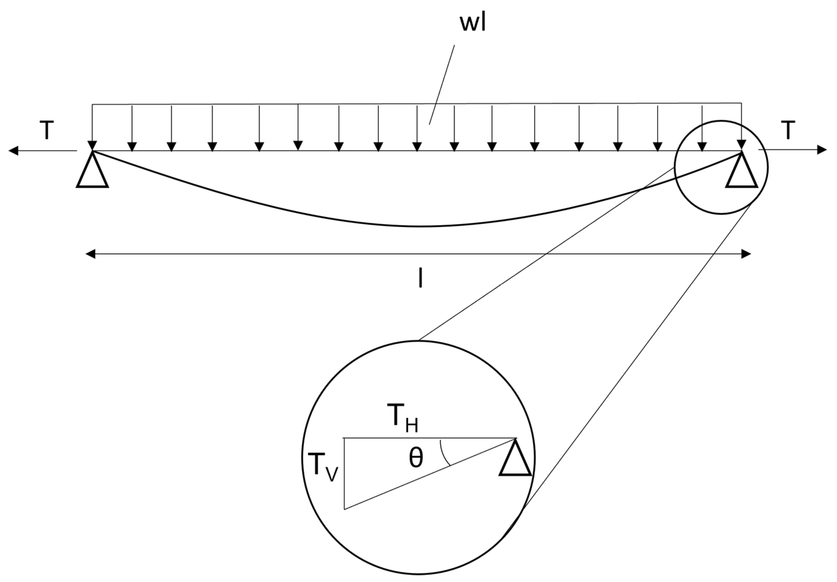
2. Description of the Developed Methos

In this section, the method used to find the expression of the maximum sag in a generic span as a function of the angle at the suspension clamp is explained. The taut cable has been modelled as a parabolic function, which is known to be sufficiently accurate for engineering purposes, excluding some special cases such as very long crossings [19]. The general case of a span with length l characterized by two supports at different levels, in which the height difference denoted as h (Figure 1), is considered. The angles at the suspension clamps are θ₁ and θ₂, while the maximum sag is f_M. Note that in the case of a span with supports at unequal levels, the maximum sag does not coincide with the vertex point of the parabola. The reference frame zero is positioned at the parabola vertex point, and x₁ and x₂ represent the horizontal coordinates of the supports A and B with respect to the reference system origin.

The first step is obtaining the expression of the maximum sag, which is the maximum vertical distance between the generic parabolic function y_P (Equation (1)) and the straight line y_R (in red) connecting points A and B of the parabola (Equation (2)).

$$y_P=k{x}^2,$$

(1)

$$y_R=k\left(x_2+x_1\right)x-k{x}_2{x}_1,$$

(2)

where k is a generic constant to take into account the mechanical parameters of the conductor. Referring to Figure 1, the relationship between x₂ and x₁ coordinates is given by Equation (3).

$$x_2=x_1+l,$$

(3)

The sag f(x), as a function of the horizontal position, is then expressed as the difference between y_P and y_R (Equation (4)).

$$f(x)=y_P-y_R=k{x}^2-k\left(x_2+x_1\right)x+k{x}_2{x}_1,$$

(4)

The goal is to find the maximum of the sag function f(x), therefore its derivative with respect to the x coordinate must be equal to zero. In this way, the coordinate of the maximum sag x_M could be found as indicated in Equation (5).

$$x_M=\frac{x_2+x_1}{2},$$

(5)

As can be appreciated, the maximum sag location is in midspan also in the case of a supports with different heights. By substituting Equation (5) in Equation (4) and making some rearrangements, a generic expression of the maximum sag f_M could be obtained (Equation (6)).

$$f_M=\frac{k{l}^2}{4},$$

(6)

At this point, the target is to express f_M as a function of one angle at the suspension clamps θ_i and of the difference between suspension height h. The tangent of the angle at the span extremity θ_i is obtained by evaluating the derivative of the parabolic function in correspondence of the x_{i (i = 1, 2)} coordinate (Equation (7)).

$$\tan {\theta }_i={\left.\frac{d{y}_p}{dx}\right|}_{x_i},$$

(7)

Using Equation (7), the expressions of x₁ and x₂ are thus obtained as functions of θ₁ and θ₂ (Equation (8)).

$$x_1=\frac{\tan {\theta }_1}{2k},\hspace{1em}\hspace{1em}{x}_2=\frac{\tan {\theta }_2}{2k},$$

(8)

Next, the height difference h can be computed as the difference between the two parabola points evaluated at the support positions (Equation (9)).

$$h=k(x_2^2-x_1^2),$$

(9)

By substituting the relationship between the x₂ and x₁ coordinates (Equation (3)) in Equation (9) and taking advantage of Equation (8), it is possible to express the constant k as function of the height difference h and one of the two suspension angles θ_i, obtaining the two expressions in Equation (10).

$$k=\frac{h}{l^2}-\frac{\tan {\theta }_1}{l},\hspace{1em}\hspace{1em}k=\frac{\tan {\theta }_2}{l}-\frac{h}{l^2},$$

(10)

In the end, the expression of the maximum sag f_M as function of h and θ₁ is obtained in Equation (11) by substituting Equation (10) in Equation (6).

$$f_M=\frac{l}{4}\left(\frac{h}{l}-\tan {\vartheta }_1\right),$$

(11)

Analogously, Equation (12) expresses the maximum sag f_M as function of h and θ₂.

$$f_M=\frac{l}{4}\left(\tan {\theta }_2-\frac{h}{l}\right),$$

(12)

It is also possible to find the expression of f_M as a function only of the two angles at the span extremities θ₁ and θ₂ by substituting the two expressions of Equation (8) into Equation (3) and rearranging the terms (Equation (13)).

$$k=\frac{1}{2l}\left(\tan {\theta }_2-\tan {\theta }_1\right),$$

(13)

Again, substituting the expression of k in Equation (6), an alternative formulation of the maximum sag f_M is obtained (Equation (14)).

$$f_M=\frac{l}{8}\left(\tan {\theta }_2-\tan {\theta }_1\right),$$

(14)

In conclusion, in the case of a span with supports at different levels, the maximum sag is function of one angle at the suspension clamp (e.g., θ₂ in the case of Equation (12)) and of the height difference h between the two supports, or it is a function of both angles at the suspension clamp. Therefore, the maximum sag f_M can be computed by measuring both angles at the two extremities (Equation (14)) or by knowing the height difference h between the supports and measuring the angle only at one extremity (Equations (11) and (12)).

Considering the case of a span with supports at the same level (h = 0), Equation (12) simplifies in Equation (15).

$$f_M=\frac{l\tan {\theta }_2}{4},$$

(15)

Since angles at the suspension clamps can be considered sufficiently small, the tangent of the angle can be approximated to the angle itself and the final expression of f_M is obtained (Equation (16)).

$$f=\frac{l\theta }{4},$$

(16)

Therefore, it was demonstrated that the maximum sag in a span with supports at the same height could be computed by measuring one of the angles at the span extremities. The same expression can be obtained more quickly through an engineering approach, explained as follows, always referring to the case of equal support levels.

The expression of the maximum sag according to the well-known “flat parabola method”, which can be found in the literature [7], is given by Equation (17).

$$f_M=\frac{w{l}^2}{8T_H},$$

(17)

where the cable weight per unit length w is modelled as a uniform distributed load along the span l and T_H represents the horizontal component of the tensile load T (Figure 2).

The vertical component of the tensile load for equilibrium on the span is given by Equation (18).

$$T_V=\frac{wl}{2},$$

(18)

If the vertical component of the tensile load is assumed to be kept constant along the span, the tangent of the angle at the suspension clamp θ can be expressed by the ratio between the vertical and horizontal components of the tensile load T_V and T_H (Equation (19)).

$$\tan \theta =\frac{T_V}{T_H},$$

(19)

By substituting Equation (18) in Equation (19) the expression of T_H can be computed (Equation (20)).

$$T_H=\frac{wl}{2\tan \theta },$$

(20)

Substituting Equation (20) into Equation (17), Equation (16) is again obtained. In conclusion, it was shown that, by means of both methods, a simple and straightforward expression for the sag estimation based on the measurement of one angle at the suspension clamp is obtained for the case of a span with levelled supports. This way, the k parameter and, consequently, the sag f_M, are calculated through geometrical quantities that are easily measurable (angle at the suspension clamp), without the need of the cable self-weight w and the horizontal component of the tensile load T_H, which are parameters difficult to obtain. An example of angular measurements necessary for the estimation on the maximum sag is proposed in Section 3. The case study of a span with levelled supports is considered in the experimental test performed at the Cable Dynamics Laboratory of Politecnico di Milano to test the efficiency of the proposed method.

3. Description of the Measurement System and Experimental Test

It was demonstrated in Section 2 that by measuring the angle at one extremity of the span (or measuring the angles at both span extremities in case of supports at unequal levels) it is possible to obtain an estimation of the maximum sag in the span. The idea proposed in this work is to carry out this measurement by taking advantage of wireless sensor nodes developed by the authors to perform vibration monitoring of high voltage transmission lines [18]. The method implemented in this system would allow to obtain an integrated monitoring tool to be used in the HVTL field. An experimental test was then arranged to assess the validity and reliability of the proposed method and of the system devoted to measure the conductor slope at one span extremity.

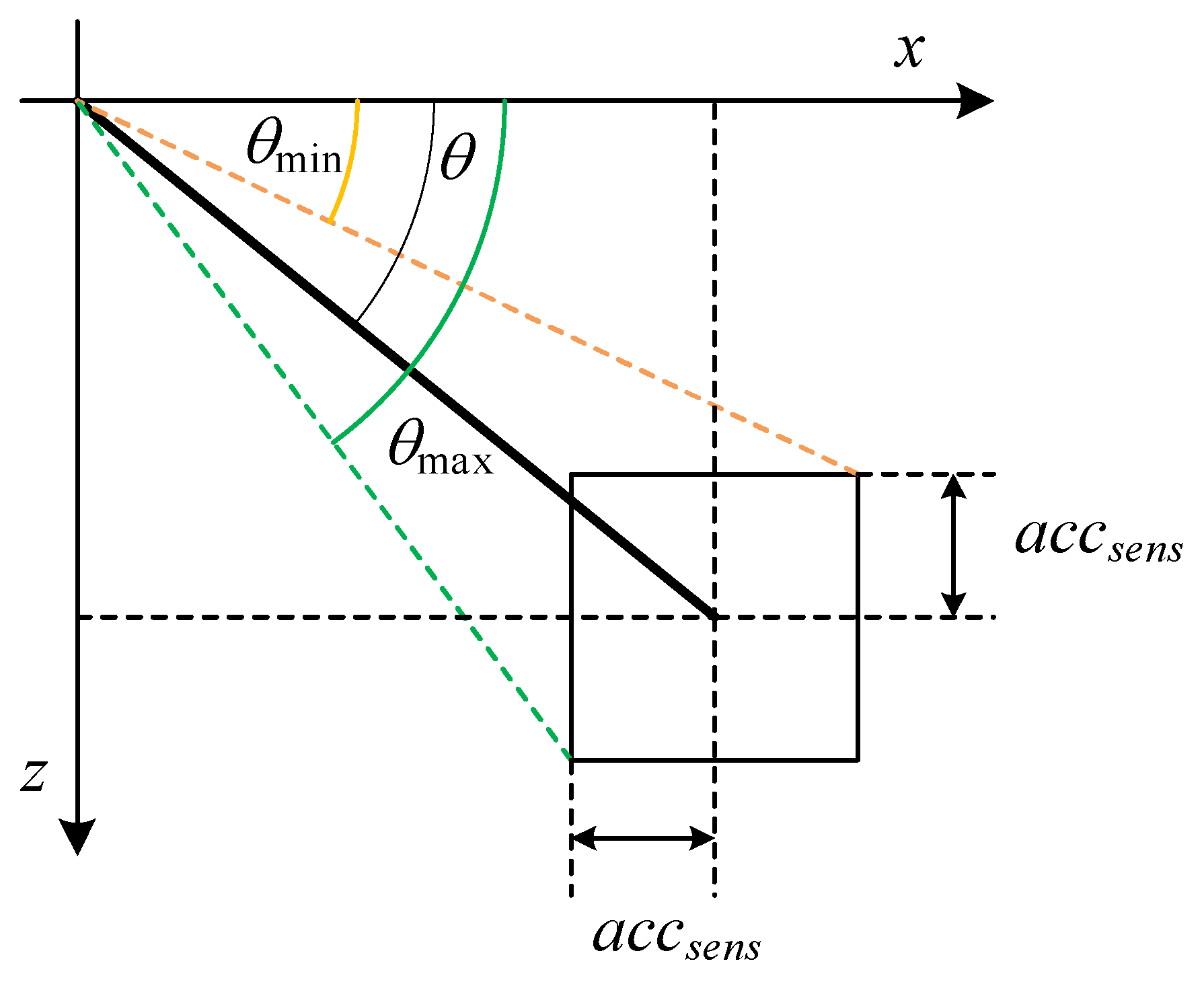
3.1. Wireless Sensor Nodes Description

A rise in the development of wireless sensors has been observed in recent years, since they allow to perform monitoring activities on mechanical structures where the installation of wired devices is not feasible, and the power supply for their operativity can be harvested from environmental sources without the need of a wired electrical supply. Examples can be found in applications developed for vibration and pressure monitoring on freight wagons [20,21], and the monitoring of wind turbines [22] and bridges [23]. Some applications of wireless sensors can also be found in the context of active control [24,25].

In the framework of HVTL, the authors developed a system composed of wireless sensor nodes to perform accelerometric measurements on HVTL conductors with the aim of obtaining, in real time, from the line, the fy_max parameter (Figure 3a), which is a fatigue indicator standardly employed in laboratory fatigue tests. Through a suitable logic, the sensor measurements can also be used to identify the different wind-induced phenomena occurring on the conductors, namely aeolian vibrations, subspan oscillations, and galloping [26]. This system is therefore employed in the field of HVTL for the estimation of the residual life of fittings and conductors and to study countermeasures for limiting the impact of wind-induced phenomena and aeroelastic effects on the structure [27,28,29].

The realized sensors are compact and light devices composed of a plastic box, a custom printed circuit board (PCB), and a rechargeable lithium battery. To reduce the measurement noise, the sensor and the clamping system have been developed with a total mass target below 1 kg. The electronic part accounts for approximately 200 g, meaning that further weight reduction can be achieved through optimizing the clamp shape. Thanks to the low power consumption and the energy inflow coming from a mini photovoltaic panel mounted on the top of the enclosure, the sensors are autonomous from the power supply point of view and can therefore be adopted for continuous monitoring in long-term campaigns.

On the PCB, several components are present. Among them, the most significant ones are a microcontroller, a Bluetooth transceiver, a temperature sensor, and a MEMS triaxial accelerometer. Since the accelerometer is a triaxial MEMS type, it allows the measurement of the acceleration static components on the three axes. This feature allows to use the accelerometer as an inclinometer, and it is therefore possible to compute the inclination angle of the device through Equation (21).

$$\theta =\arctan \left(\frac{a_x}{\sqrt{a_y{}^2+a_z{}^2}}\right)\frac{180}{\pi },$$

(21)

where a_x, a_y, and a_z are the static acceleration components with the reference system shown in Figure 3b. As can be observed, the angle to be measured for the sag estimation lays in the x–z plane (vertical plane).

The accelerometer’s main features are listed in

Table 1. Main characteristics of the MEMS accelerometer adopted for the sensor nodes.

Parameter	Value
Measurement range	±2 g, ±4 g, ±8 g, ±16 g
Sensitivity (acc_sens)	4 mg
Noise	1.1 LSB rms
Maximum output data rate	3200 Hz
Operating voltage	3.3 V
Supply current	140 µA
Operating temperature range	−40 ÷ 85 °C

, while a complete description of the sensors can be found in [30,31]. The idea at the basis of this paper is to take advantage of the versatility of these devices already employed in the field of HVTL for monitoring sag with continuity in time.

3.2. Experimental Set-Up

To test the method efficiency, an experimental set-up was arranged. To this aim, a 50 m long cable strand was tensioned in the Cable Dynamics Laboratory of Politecnico di Milano. The Cable Dynamics Laboratory is mainly used for evaluating the mechanical properties of cable and damping devices, namely the conductor self-damping, the damper, and the spacer-damper dynamic stiffness and damping properties [32]. The knowledge of these parameters allows to correctly estimate, through numerical models, the HVTL dynamic response to the wind action.

The peculiar features of the facility are the 50 m long span, which represents a strict requirement for many tests performed by standards, and the presence of an electromechanical actuator and a load cell, which permit to easily control and regulate the conductor tensile load.

The instrumentation available in the laboratory comprises an electrodynamic shaker used to excite the cable vibration and some current suppliers (for a total power of 50 kW) to perform conductor heating and thermal tests.

The cable employed for the tests is a high temperature low sag (HTLS) conductor characterized by an external diameter of 30.45 mm. The main features of the cable are summed up in

Table 2. Main characteristics of the conductor employed in the tests.

Conductor Characteristics
External diameter	30.45 mm
Mass per unit length	1.485 kg/m
Ultimate tensile strength (UTS)	180 kN
Maximum operative temperature	120 °C

.

One sensor node was used for the tests, and was mounted at a distance sufficiently high (i.e., approximately 1 m) from the conductor extremity to avoid the zone influenced by the high bending stiffness due to the presence of the clamp (Figure 4a). The sensor node acquisition was ruled by a gateway positioned in the laboratory, which continuously stored the received data.

The tensile load of the conductor was imposed and controlled by means of programmable logic control (PLC) managing the electromechanical actuator and the load cell. A linear position sensor (Celesco encoder model PT5A-100-S47-FR-10K-M6 with a sensitivity of 265 mm/V) was used to measure, with accuracy, the sag at the midspan during the different tests illustrated in the following sections (Figure 4b).

3.3. Tests Description

Purpose of the experimental activities was to compare the sag value, estimated with the proposed method based on the sensor node angular measurements, and the actual reference value, measured through the linear position sensor. Essentially, two test sessions were carried out, decreasing step-by-step the value of the tensile load in the first one and increasing it in the second one (

Table 3. Tests performed in the Cable Dynamics Laboratory.

Test Number	Initial Tensile Load	Final Tensile Load
Test 1	40 kN (22.2% UTS)	5 kN (2.8% UTS)
Test 2	6 kN (3.3% UTS)	40 kN (22.2% UTS)

). For each session, several steps were performed to obtain, as much as possible, a continuous curve of the sag value as a function of the tensile load tested. The scope of the tests was also to verify a possible dependence of the sag estimation on the tensile load, namely, if the estimation was rougher for low tensile load values. The higher tensile load tested (40 kN) corresponds to approximately the 22% of the cable UTS, which represents a common value adopted in operative conditions. The lower value tested (5 kN) was the minimum acceptable before reaching an excessively low sag value (the cable would have touched the ground).

For each tensile load tested, the following parameters were obtained: the angle measured by the wireless sensor through Equation (21), the tensile load imposed to the cable, and the actual sag at midspan.

During the tests, a progressive torsion of the cable occurring with the tensile load variation was observed. This behavior justifies the adoption of a MEMS triaxial accelerometer, which allows to compensate for the rotation (through the measurement of the lateral static acceleration a_y) and to geta reliable angular measurement. The results obtained from the experimental tests are presented in the following section.

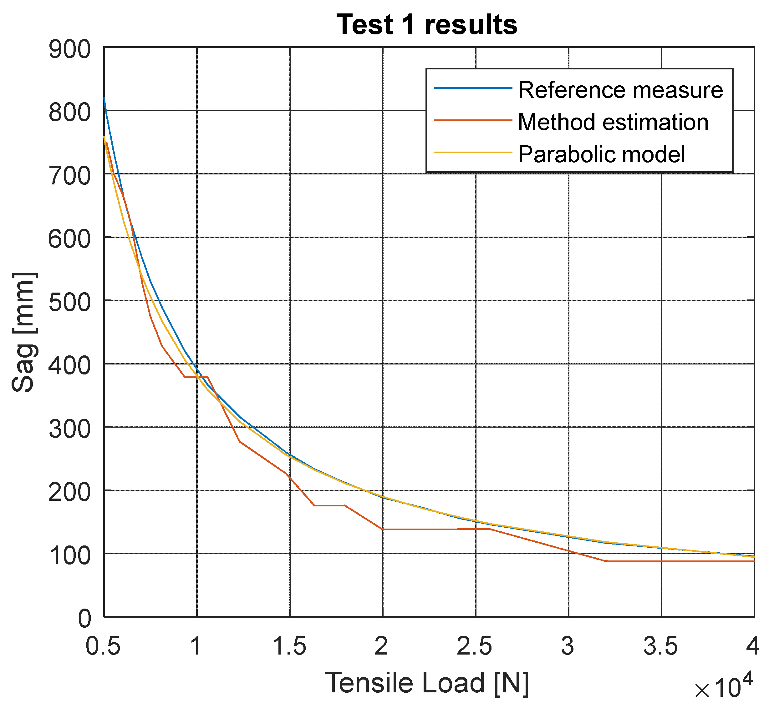
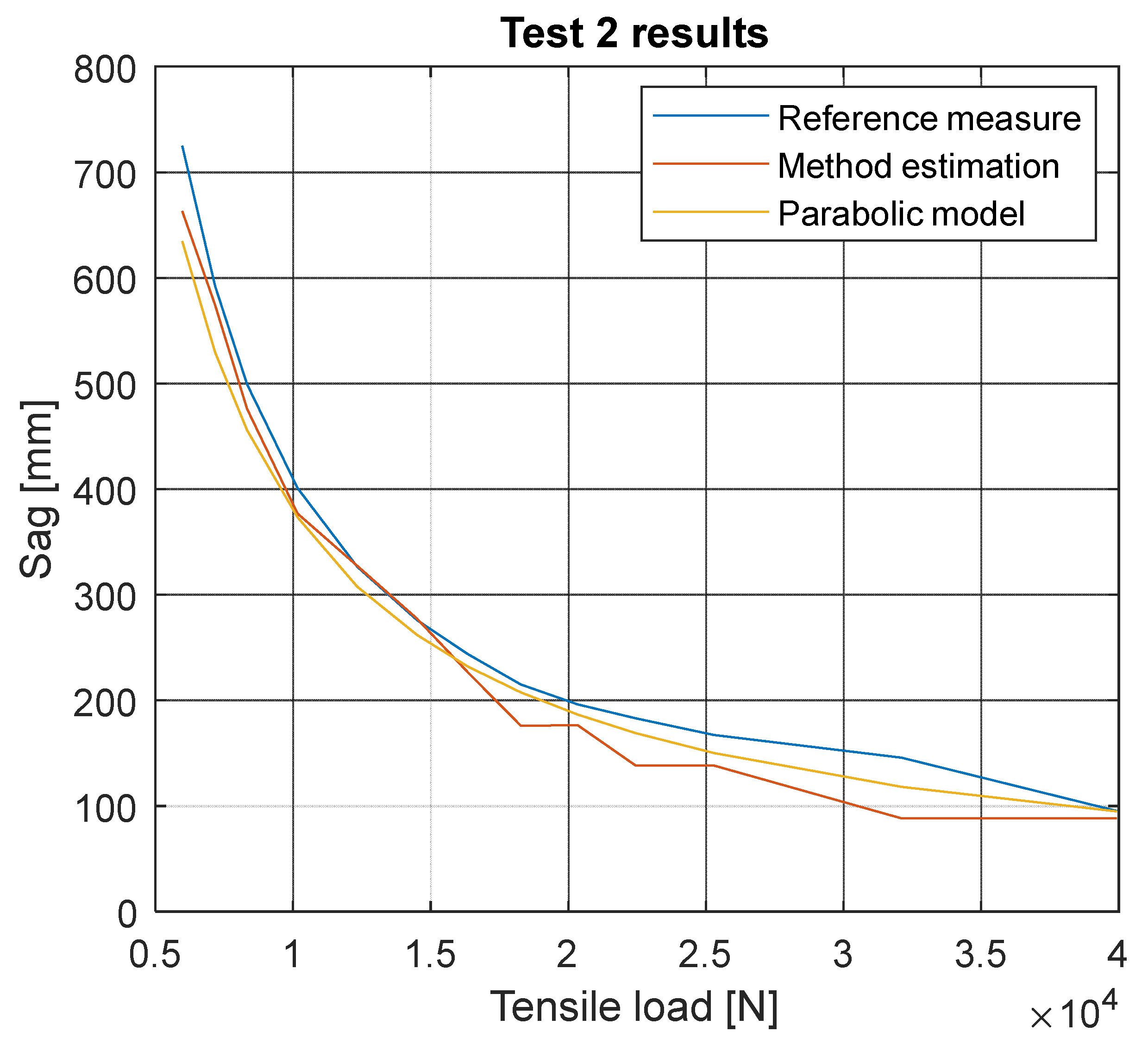
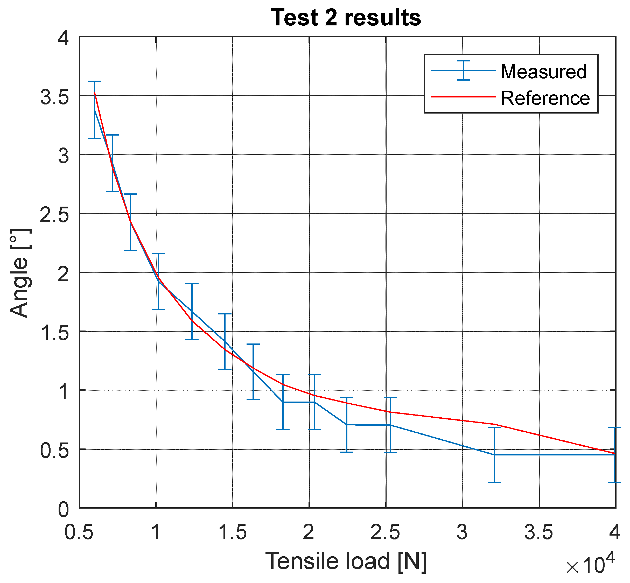
4. Results and Discussion

The main outcome of the experimental activities described in Section 3 is represented by the estimation of the sag, as a function of the tensile load imposed to the cable, by means of the proposed method and the wireless sensors for the angular measurements. Estimated values (red curve in Figure 5) are compared with sag values measured through the linear position sensors installed at the midspan, which are taken as reference values (blue curve). The third curve (yellow curve) plotted represents the sag obtained with the classical formulation, which approximates the cable as a parabolic curve (Equation (1)), having considered known the tensile load imposed to the cable.

The focus is firstly put on the sag curve computed through the parabolic expression assuming the known tensile load value (yellow curve). This curve is nearly superimposed to the curve of measured reference sag values up to very low tensile loads, where a slight discrepancy can be observed. On the other hand, the proposed method allows to obtain a satisfactory prediction of the sag trend varying the tensile load. However, in some cases, a difference between estimated and measured values is present. This behavior, particularly noticeable at higher tensile loads where the sag variation is lower from step to step, can be explained by analyzing the angle values estimated through the proposed method. Since the sag is directly proportional to the angle apart from a constant (Equation (16)), the curve presents the same trend of sag one as visible in Figure 6. In this case, the angle at the span extremity measured by the sensor (blue curve) and the angle evaluated through the catenary equation in the same position on the basis of the sag measured as reference (red curve) are compared [33].

In this case, error bars reported on the measured angle curve θ_mis (blue curve) represent the maximum errors made by the sensor in the measurement phase and were computed through Equation (22).

$$\theta ={\theta }_{mis}\pm \frac{\Delta \theta }{2},$$

(22)

where Δθ is the difference between the maximum and minimum measurable angles θ_max and θ_min according to Equation (23).

$$\Delta \theta ={\theta }_{max}-{\theta }_{min},$$

(23)

The maximum and minimum measurable angles θ_max and θ_min are a function of the accelerometer resolution acc_sens, according to Figure 7, and are computed, respectively, through Equations (24) and (25). The value of acc_sens is reported among the accelerometer main features in Table 1.

$${\theta }_{max}=\arctan \left(\frac{\sin \theta +ac{c}_{sens}}{\cos \theta -ac{c}_{sens}}\right),$$

(24)

$${\theta }_{min}=\arctan \left(\frac{\sin \theta -ac{c}_{sens}}{\cos \theta +ac{c}_{sens}}\right),$$

(25)

This error may vary depending on the angle’s actual value. However, since the angle value is always small in the performed tests, the error can be considered constant along all the range of interest.

As can be noticed in Figure 6, the reference curve lays in between the measured one and the error bars, meaning that measurements are consistent with the expected sensor behavior. Nonetheless, an accelerometer with a better amplitude resolution would have allowed to reproduce the sag trend with more accuracy.

A similar behavior is visible by analyzing Test 2 results, reported in the sag comparison (Figure 8) and angle comparison (Figure 9). The main purpose of Test 2 was the possible detection of different cable behaviors in terms of the sag-angle relationship during a step-by-step increasing of tensile load (instead of decreasing it, as in Test 1).

Again, a higher discrepancy can be observed at higher tensile loads, where smaller angles must be detected by the sensor. The solution can be improved in these terms, as already pointed out previously, by adopting a MEMS accelerometer characterized by a higher amplitude resolution. An example can be represented by the IIM-42351 from TDK InvenSense, which allows an amplitude resolution up to 0.5 mg (using the ±2 g full scale range). Despite of this, the validity of the proposed method in detecting the sag variation using angular measurements carried out with wireless sensors was verified with experimental tests. Therefore, the developed system can represent an integrated, low-cost, and robust solution to be used both for vibration monitoring of wind-induced phenomena on conductors and for sag monitoring during the line operativity.

5. Conclusions

In this work, a simple method to estimate the sag value by measuring the conductor slope at the span extremities was derived. The proposed solution can be adopted for both cases of span with supports at equal or different heights. The main advantage of the method is that the parameters needed for the sag estimation are geometrical quantities easily measurable on an operative line. The angle measurement is performed by means of wireless sensors developed by the authors and adopted in the field for the monitoring of wind-induced vibrations occurring on HVTL conductors. These sensors are endowed with a MEMS accelerometer, which is used, in this case, essentially as an inclinometer. A laboratory test was arranged to demonstrate the ease of implementing the proposed solution. The test on a real cable allowed to check the efficiency of the method and the monitoring system in obtaining a sag estimation from angular measurements for different tensile loads imposed to the cable. Through data analysis and comparison with reference values, it was then demonstrated that the solution proposed is suitable to the scope, and represents a low-cost, easy to install, and robust system to perform a complete set of monitoring activities in the field of HVTL.

References

1. EPRI. EPRI: Transmission Line Reference Book: Wind-Induced Conductor Motion, 2nd ed.; EPRI: Washington, DC, USA, 2009. [Google Scholar]
2. Kiessling, F.; Nefzger, P.; Nolasco, J.F.; Kaintzyk, U. Overhead Power Lines—Planning, Design, Construction; Springer: Berlin, Germany, 2003; Volume 759. [Google Scholar]
3. Castillo, V.Z.; de Boer, H.S.; Muñoz, R.M.; Gernaat, D.E.H.J.; Benders, R.; van Vuuren, D. Future global electricity demand load curves. Energy 2022, 258, 124741. [Google Scholar] [CrossRef]
4. Riba, J.R.; Bogarra, S.; Gómez-Pau, Á.; Moreno-Eguilaz, M. Uprating of transmission lines by means of HTLS conductors for a sustainable growth: Challenges, opportunities, and research needs. Renew. Sustain. Energy Rev. 2020, 134, 110334. [Google Scholar] [CrossRef]
5. Silva, A.A.P.; Bezerra, J.M.B. Applicability and limitations of ampacity models for HTLS conductors. Electr. Power Syst. Res. 2012, 93, 61–66. [Google Scholar] [CrossRef]
6. Karimi, S.; Musilek, P.; Knight, A.M. Dynamic thermal rating of transmission lines: A review. Renew. Sustain. Energy Rev. 2018, 91, 600–612. [Google Scholar] [CrossRef]
7. Hu, Y.; Liu, K. Inspection and Monitoring Technologies of Transmission Lines with Remote Sensing; Academic Press: Cambridge, MA, USA, 2017; ISBN 9780128126448. [Google Scholar]
8. Mahin, A.U.; Islam, S.N.; Ahmed, F.; Hossain, M.F. Measurement and monitoring of overhead transmission line sag in smart grid: A review. IET Gener. Transm. Distrib. 2022, 16, 1–18. [Google Scholar] [CrossRef]
9. Kamboj, S.; Dahiya, R. Application of GPS for SAG measurement of overhead power transmission line. Int. J. Electr. Eng. Inform. 2011, 3, 268–277. [Google Scholar] [CrossRef]
10. Zengin, A.T.; Erdemir, G.; Akinci, T.C.; Seker, S. Measurement of Power Line Sagging Using Sensor Data of a Power Line Inspection Robot. IEEE Access 2020, 8, 99198–99204. [Google Scholar] [CrossRef]
11. Wydra, M.; Kisala, P.; Harasim, D.; Kacejko, P. Overhead transmission line sag estimation using a simple optomechanical system with chirped fiber bragg gratings. part 1: Preliminary measurements. Sensors 2018, 18, 309. [Google Scholar] [CrossRef] [Green Version]
12. Godard, B. A vibration-sag-tension-based icing monitoring of overhead lines. Int. Work. Atmos. Icing Struct. 2019, 1, 1–7. [Google Scholar]
13. Sacerdotianu, D.; Nicola, M.; Nicola, C.I.; Lazarescu, F. Research on the continuous monitoring of the sag of overhead electricity transmission cables based on the measurement of their slope. In Proceedings of the 2018 International Conference on Applied and Theoretical Electricity (ICATE), Craiova, Romania, 4–6 October 2018; pp. 1–5. [Google Scholar] [CrossRef]
14. Verma, S.; Rana, P. Wireless communication application in smart grid: An overview. In Proceedings of the 2014 Innovative Applications of Computational Intelligence on Power, Energy and Controls with their impact on Humanity (CIPECH), Ghaziabad, India, 28–29 November 2014; pp. 310–314. [Google Scholar] [CrossRef]
15. Malhara, S.; Vittal, V. Mechanical state estimation of overhead transmission lines using tilt sensors. IEEE Trans. Power Syst. 2010, 25, 1282–1290. [Google Scholar] [CrossRef]
16. Xiao, X.; Xu, Y.; Zhang, J.; Xu, K. Research on Sag Online Monitoring System for Power Transmission Wire Based on Tilt Measurement. Int. J. Smart Grid Clean Energy 2013, 2, 6–11. [Google Scholar] [CrossRef] [Green Version]
17. Hayes, R.M.; Nourai, A. Power Line Sag Monitor. U.S. Patent 6,205,867 B1, 26 March 2001. [Google Scholar]
18. Zanelli, F.; Mauri, M.; Castelli-Dezza, F.; Tarsitano, D.; Manenti, A.; Diana, G. Analysis of Wind-Induced Vibrations on HVTL Conductors Using Wireless Sensors. Sensors 2022, 22, 8165. [Google Scholar] [CrossRef]
19. CIGRE: Study Committee B2: Overhead Lines. Green Book: Overhead Lines; Springer: Cham, Switzerland, 2017; ISBN 978-3-319-31747-2. [Google Scholar]
20. Zanelli, F.; Mauri, M.; Debattisti, N.; Castelli-dezza, F.; Sabbioni, E.; Tarsitano, D. Energy Autonomous Wireless Sensor Nodes for Freight Train Braking Systems Monitoring. Sensors 2022, 22, 1876. [Google Scholar] [CrossRef]
21. Zanelli, F.; Sabbioni, E.; Carnevale, M.; Mauri, M.; Tarsitano, D.; Castelli-Dezza, F.; Debattisti, N. Wireless sensor nodes for freight trains condition monitoring based on geo-localized vibration measurements. Proc. Inst. Mech. Eng. Part F J. Rail Rapid Transit 2023, 237, 193–204. [Google Scholar] [CrossRef]
22. Alves, M.M.; Pirmez, L.; Rossetto, S.; Delicato, F.C.; de Farias, C.M.; Pires, P.F.; dos Santos, I.L.; Zomaya, A.Y. Damage prediction for wind turbines using wireless sensor and actuator networks. J. Netw. Comput. Appl. 2017, 80, 123–140. [Google Scholar] [CrossRef]
23. Chae, M.J.; Yoo, H.S.; Kim, J.Y.; Cho, M.Y. Development of a wireless sensor network system for suspension bridge health monitoring. Autom. Constr. 2012, 21, 237–252. [Google Scholar] [CrossRef]
24. Debattisti, N.; Bacci, M.L.; Cinquemani, S. Distributed wireless-based control strategy through Selective Negative Derivative Feedback algorithm. Mech. Syst. Signal Process. 2020, 142, 106742. [Google Scholar] [CrossRef]
25. Debattisti, N.; Bacci, M.L.; Cinquemani, S. Implementation of a partially decentralized control architecture using wireless active sensors. Smart Mater. Struct. 2020, 29, 025019. [Google Scholar] [CrossRef]
26. Diana, G.; Tarsitano, D.; Mauri, M.; Castelli-Dezza, F.; Zanelli, F.; Manenti, A.; Ripamonti, F. A wireless monitoring system to identify win induced vibrations in HV transmission lines. In Proceedings of the 3rd SEERC Conference, Vienna, Austria, 29 November–2 December 2021. [Google Scholar]
27. Argentini, T.; Rocchi, D.; Somaschini, C.; Spinelli, U.; Zanelli, F.; Larsen, A. Journal of Wind Engineering & Industrial Aerodynamics Aeroelastic stability of a twin-box deck: Comparison of different procedures to assess the effect of geometric details. J. Wind Eng. Ind. Aerodyn. 2022, 220, 104878. [Google Scholar] [CrossRef]
28. Godard, B.; Guerard, S.; Lilien, J.L. Original real-time observations of aeolian vibrations on power-line conductors. IEEE Trans. Power Deliv. 2011, 26, 2111–2117. [Google Scholar] [CrossRef]
29. Diana, G.; Belloli, M.; Giappino, S.; Manenti, A.; Mazzola, L.; Muggiasca, S.; Zuin, A. A numerical approach to reproduce subspan oscillations and comparison with experimental data. IEEE Trans. Power Deliv. 2014, 29, 1311–1317. [Google Scholar] [CrossRef]
30. Zanelli, F.; Castelli-Dezza, F.; Tarsitano, D.; Mauri, M.; Bacci, M.L.; Diana, G. Sensor Nodes for Continuous Monitoring of Structures Through Accelerometric Measurements. In Proceedings of the 2020 IEEE International Workshop on Metrology for Industry 4.0 & IoT, Roma, Italy, 3–5 June 2020; pp. 152–157. [Google Scholar] [CrossRef]
31. Zanelli, F.; Castelli-Dezza, F.; Tarsitano, D.; Mauri, M.; Bacci, M.L.; Diana, G. Design and field validation of a low power wireless sensor node for structural health monitoring. Sensors 2021, 21, 1050. [Google Scholar] [CrossRef] [PubMed]
32. Diana, G.; Falco, M.; Cigada, A.; Manenti, A. On the measurement of transmission line conductor self-damping. In Proceedings of the IEEE PES Winter Meeting, New York, NY, USA, 31 January–4 February 1999. [Google Scholar]
33. Hatibovic, A. Derivation of equations for conductor and sag curves of an overhead line based on a given catenary constant. Period. Polytech. Electr. Eng. Comput. Sci. 2014, 58, 23–27. [Google Scholar] [CrossRef] [Green Version]
Figure 1. Schematization of the span with unequal level supports with a parabolic function. Angles are positive when describing a counterclockwise rotation.
Applsci 13 03175 g001
Figure 2. Schematic representation of a conductor span of length l modelled according to the “flat parabola method”.
Applsci 13 03175 g002
Figure 3. Wireless sensors developed for vibration monitoring of HVTL conductors: (a) Three sensors mounted on conductors of an operative HVTL; (b) Reference system of the triaxial MEMS accelerometer equipping wireless sensors.
Applsci 13 03175 g003
Figure 4. Experimental set-up arranged in the Cable Dynamics Laboratory: (a) Sensor node positioned at one extremity to carry out angular measurement; (b) Linear position sensor placed at midspan to obtain the reference value of maximum sag.
Applsci 13 03175 g004
Figure 5. Comparison of the sag values estimated through the proposed method (red curve) with the reference measured values (blue curve) and the ones from the parabolic model (yellow curve) during Test 1.
Applsci 13 03175 g005
Figure 6. Comparison between the angle values measured by the sensors and the reference ones computed through catenary equation in correspondence of the sensor position during Test 1. Error bars represent the uncertainty of the sensor measurements.
Applsci 13 03175 g006
Figure 7. Schematization of angles in the vertical plane for the computation of θmax and θmin, used to obtain the sensor uncertainty.
Applsci 13 03175 g007
Figure 8. Comparison of the sag values estimated through the proposed method (red curve) with the reference measured values (blue curve) and the ones from the parabolic model (yellow curve) during Test 2.
Applsci 13 03175 g008
Figure 9. Comparison between the angle value measured by the sensors and the reference one computed through catenary equation in correspondence of the sensor position during Test 2. Error bars represent the uncertainty of the sensor measurements.
Applsci 13 03175 g009