Analytical Prediction of Tunnel Deformation Beneath an Inclined Plane: Complex Potential Analysis

Abstract

When excavating a tunnel, the stresses are distributed asymmetrically along the tunnel cross-section. Other factors, particularly slope friction force and excavation speed, can also contribute to the deformation and displacement of a tunnel. Despite this, several authors have used the complex potential method to predict the ground deformation surrounding the tunnel. However, their applicability to the ground response caused by the asymmetric stress distribution around the tunnel wall is analysed in this context. This paper, therefore, proposes an approximate solution on the slope to predict the tunnel cross-section deformation. The solution is based on the complex potential method to predict analytically and numerically the ground deformation around the tunnel. However, two variables called the “complex potential functions” for the Laurent series expansion are used for the stress redistribution to the tunnel boundary conditions. Data from the Qijiazhuang tunnel case are used to justify the proposed analytical solutions. This solution is an essential guide for analyzing deformations in complex geological conditions and structures, such as steeper slopes.

1. Introduction

Estimating the loads on the ground surface before and after tunnel excavation is an essential concept in current engineering. The prediction of the ground deformation of a tunnel under a slope can be interpreted both analytically and numerically. Using analytical solutions to determine the stresses and displacements around the tunnel is also practical [1]. Indeed, it is essential to recognize the substantial impact of excavation and assisted construction procedures and their technical details on the distribution of stresses/deformations around the opening and its digital support system.

Methods for predicting ground motion fall primarily into three categories: empirical methods [2,3,4,5,6,7,8], numerical methods [9,10,11,12,13,14,15] and finally, analytical methods [14,16,17,18,19,20,21,22,23,24,25,26,27,28,29,30,31].

Furthermore, other approaches based on an approximation of the Navier–Stokes equations (for incompressible materials at the free surface) are proposed, taking into account the absence of hydrostatic equilibrium, assuming that the medium has a small temperature variation [32]. Thus, according to Jong et al. [33], the unique mechanical properties of the contact surface can then have a large influence on the deformation of the soil, thus interacting with the soil–structure contact. The soil response can be described not only by the soil failure states but also by the material stiffness. The mode of displacement of the wall (all buried materials) greatly influences the intensity and distribution of the compression pressure. In execution, different theories may be applicable, justified and verified by the assumption that the soil properties, the roughness of the structure, and the state of ground deformation may be admitted in the plastic or non-plastic domain.

Depending on the excavation depth, many studies have been conducted on shallow tunnels, but few on sloping tunnels have been presented. Until now, some research has focused on the effect of non-uniform deformation caused by ground loss, offering estimations of the motion imposed by various deformation models associated with the open tunnel [26,28,31,34,35,36,37]. Furthermore, Kong et al. [15] propose a unified displacement function to express by Fourier series a more detailed description of the deformation mode of a shallow circular tunnel cross-section when the ground surface is sloping. These various methods are based on linear elasticity theory in order to simplify the fixed stress shapes at the lower limit of the tunnel. These approaches can also be utilized to simultaneously determine the tunnel stresses and displacements when the tunnel is sloping.

Recently, many engineers have used analytical approaches to predict the deformation of the ground surrounding a tunnel. Their applicability to the stability of a tunnel under a slope is less developed. Therefore, this paper presents an approximate solution based on the complex variable method to predict the tunnel deformation beneath a slope. The method is based on two parameters called “complex potential functions” ($\phi \left(z\right)$, $\Psi \left(z\right)$), also known as “Goursat functions”. The main idea is to obtain solutions to the deformation of the tunnel wall using the complex potential function under an acceptable limit. More precisely, at the boundary conditions, the stresses applied to the tunnel wall are evaluated as a function of the variation of the surface load while measuring the boundary stress and the displacement of the cross-section by combining the stress-displacement terms. Thus, analytically, the left and right infinite boundaries define the two complex displacement functions when developing the Laurent series. The displacement model is then integrated with the complex potentials to analytically predict the deformation induced by the inclined plane. The performance and viability of this method are explored using a series of analyses introduced by the complex displacement. Monitoring data from the Qijiazhuang tunnel in China is used to justify the results presented by the analytical formulas.

2. Tunnel Description Beneath a Slope

The geometric representation of Figure 1 depicts a model of a shallow tunnel beneath an inclined plane (infinite domain) in a two-dimensional Cartesian plane with coordinates ($x$,$y$); angle of inclination $\beta$; a central axis of the tunnel $o_1$; varying equilibrium depths $h_1$ and $h_2$ (left and right), respectively, where$h$ is the central depth of the tunnel; and a radial distance from the tunnel axis$r$. The tunnel boundary condition provides a compression force between the inner pressure $p_0$ and the outer pressure $p_1$ under the effect of the slope. Because the tunnel is excavated under a slope, the friction force $F_f$ is considered (Figure 1). The Airy stress function ($U$) is used in two-dimensional functions to evaluate the asymmetric stress distribution on the ground surface. The general form of the solution is deduced from the biharmonic function term. Following the biharmonic function, we can obtain${\nabla }^2{\nabla }^{2}U=0$. The general equation resulting from the biharmonic function in the term of analytical function is written as follows:

$$f_{\left(z\right)}=C+iD$$

(1)

where$f_{\left(z\right)}$ is the analytical function and C and D are real functions that satisfy the Cauchy–Riemann condition. A function$\phi \left(z\right)$ introduced by integrating$f_{\left(z\right)}$,$\phi \left(z\right)$ can be written as follows: $\phi \left(z\right)=c+id$ with $\partial \phi /\partial z=\partial c/\partial x+i\partial d/\partial y=1/4\left(C+iD\right)$. Considering the function

$$F=U=\frac{1}{2}\left(x-iy\right)\left(c+id\right)-\frac{1}{2}\left(x+iy\right)\left(c-id\right)=Re \left(\chi \left(z\right)\right)$$

(2)

where χ(z) is given in Appendix A, and $x$ and $y$ are shown in Appendix C, $\chi \left(z\right)$ is another analytical function of $z$ and the imaginary part $\chi \left(z\right)$ can be denoted G, hence, $\chi \left(z\right)=F+iG$. Following Equation (2), the Airy stress function can be redefined as (Figure 2):

$$U=\frac{1}{2}\left(\overline{z}\phi \left(z\right)+z\overline{\phi \left(z\right)}+\chi \left(z\right)+\overline{\chi \left(z\right)}\right)$$

(3)

where Figure 2 is shown as follows: (a) uniform convergence, (b) ovalization, (c) translation movement and (d) final shape of the displacement. Equation (3) is a general formula of the biharmonic equation. Under the influence of the slope, the subsequent section will generate the stresses and displacements surrounding the tunnel.

3. Mathematical Analysis

3.1. Asymmetric Stress around the Tunnel

With population growth, many engineers are tunnelling under the slope. This causes an asymmetric stress distribution on the tunnel wall. The stress on the ground surface is determined by the compression load between the tunnel wall and the slope surface. Using the stress in term of the Airy stress function, Equation (2) can be rewritten as follows:

$$F=F_1+i{F}_2=U-xc-yd$$

(4)

where$F$,$c$,$d$ are the harmonic function. The proposed expressions in Equation (3) can be found in Equation (A1). The final displacement can be proposed in the form:

$$\frac{{\partial }^{2}U}{\partial x^2}+i\frac{{\partial }^{2}U}{\partial y\partial x}=z\overline{{\phi }^{″}\left(z\right)}+{\phi }^{\prime }\left(z\right)+\overline{{\phi }^{\prime }\left(z\right)}+\overline{{\Psi }^{\prime }\left(z\right)}$$

(5)

where φ’(z) is illustrated in Appendix A.

According to the Kolosov–Muskhelishvili method, the formulas offer the best method to treat the 2D crack problem (Equation (A1)). The force applied (Equation (A2)) can result in regular and continuous displacements [38]. The stress described by the Airy function can be given as follows:

$${\sigma }_{xx}+{\sigma }_{yy}=2\left({\phi }^{\prime }\left(z\right)+\overline{\phi \left(z\right)}\right)$$

(6)

$${\sigma }_{yy}-{\sigma }_{xx}+2i{\tau }_{xy}=2\left\{\overline{z}{\phi }^{″}\left(z\right)+{\Psi }^{\prime }\left(z\right)\right\}$$

(7)

Equations (6) and (7) indicate the complex potential of the stress. Hence, the stress derivatives give ${\sigma }_{xx}={\partial }^{2}U/\partial x^2$ (horizontal stress), ${\sigma }_{yy}={\partial }^{2}U/\partial y^2$ (vertical stress) and${\tau }_{xy}={\partial }^{2}U/\partial x\partial y$ (shear stress).

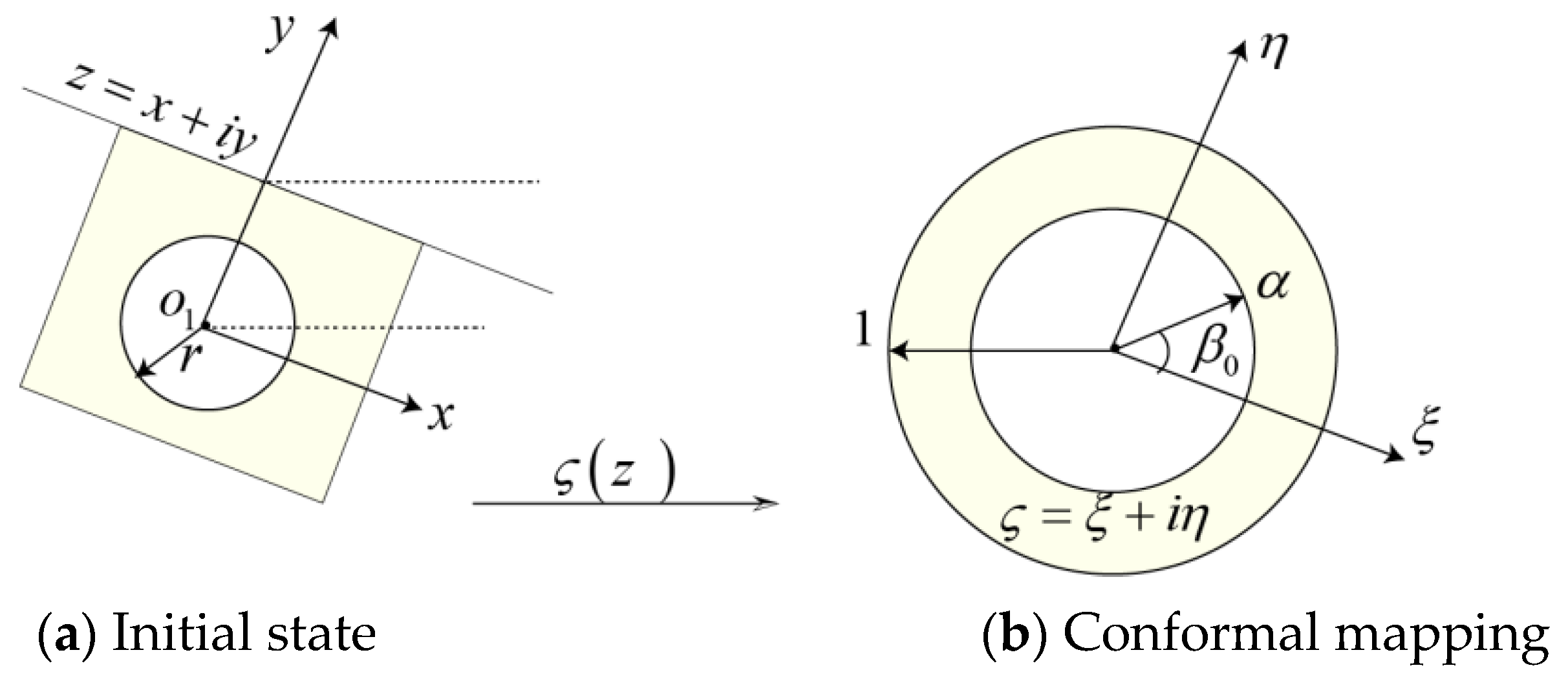
3.2. Complex Potential Analysis

3.2.1. Exact Solution

Muskhelishvili [39] demonstrated that the complex potential method relies on the theory of linear elasticity in a deformation field. The elastic half-plane is not constantly stretched, which is a shortcoming of this complex and rigorous solution [20]. Using the complex potential functions $\phi \left(z\right)$ and $\Psi \left(z\right)$ of Muskhelishvili [39], Mitchell [40] solved a stress concentration problem for a doubly symmetric hole whose boundary consists of three crossed circles. The method enables the evaluation of complex tunnel wall stresses and displacements. The method is implemented on two systems of “complex potential functions” $\phi \left(z\right)$ and $\Psi \left(z\right)$. The displacement is related to the analytical function established in Equation (8),

$$2\mu \left(u_x+i{u}_y\right)=k_0\phi \left(z\right)-z\overline{\frac{\partial \phi }{\partial z}}-\overline{\Psi \left(z\right)}$$

(8)

where $k_0=3-4v$ is the elastic constant, $u_x$ is the horizontal displacement, $u_y$ is the vertical displacement and $\mu$ is the shear modulus ($z \overline{\partial \phi }$/$\partial z$ and $\overline{\Psi \left(z\right)}$ are shown in Appendix A). At the boundary condition, the necessary solution to the deformation is to evaluate the horizontal and vertical displacement of the ground around the tunnel. For deformation problems related to the surface traction boundary condition, the displacement can be represented in the complex $z-$ plane (Figure 3a). The first step is based on the complex displacement, usually defined by Equation (8). The second step is described by stresses ${\sigma }_{xx}-i{\sigma }_{yy}$ and ${\sigma }_{yy}+i{\tau }_{xy}$. A space $r$ in an annular $z-$ plane is mapped into a $\varsigma -$ plane, bounded by a circle $\left|\varsigma \right|=$1 and $\left|\varsigma \right|=\alpha$ (Figure 3b). The general transcription of the complex forces is developed based on the Laurent series. The conformal transformation is defined by:

$$z=\omega \left(z\right)=ih\frac{1-{\alpha }^2}{1+{\alpha }^2}\frac{1+\varsigma }{1-\varsigma }$$

(9)

where the derivation ${\omega }^{\prime }\left(\varsigma \right)=2ih\left(1-{\alpha }^2\right)/\left(1-\varsigma \right)\left(1+{\alpha }^2\right)$, $\varsigma$ is the mapped complex coordinate, $h=r\left(1+\alpha \right)/2\alpha$ ($\alpha$ is the embedment ratio parameter) and $r^2=x^2+{\left(y+h\right)}^2$. Hence, the Goursat parameter can be expressed as:

$$\phi \left(z\right)=\phi \left(\omega \left(\varsigma \right)\right)={\phi }_0\left(\varsigma \right)$$

(10)

$$\Psi \left(z\right)=\Psi \left(\omega \left(\varsigma \right)\right)={\Psi }_0\left(\varsigma \right)$$

(11)

The derivation of $\phi \left(z\right)$ can be obtained by$\partial \phi /\partial z=\partial \phi /\partial \varsigma .\partial \varsigma /\partial z={\phi }_0\left(\varsigma \right)/\overline{{\omega }^{\prime }\left(\varsigma \right)}$. When $\left|\varsigma \right|=1$ and $\left|\varsigma \right|=\alpha$ are transformed into a $\varsigma -$ space, Equations (10) and (11) could be established as follows:

$$\left|\varsigma \right|=1; {\phi }_0\left(\varsigma \right)+\frac{\omega \left(\varsigma \right)}{\overline{{\omega }^{\prime }\left(\varsigma \right)}}\overline{{{\phi }^{\prime }}_0\left(\varsigma \right)}+\overline{{\Psi }_0\left(\varsigma \right)}=0;$$

(12)

$$\left|\varsigma \right|=\alpha ; {\mathsf{\phi }}_0\left(\mathsf{\varsigma }\right)-\frac{\mathsf{\omega }\left(\mathsf{\varsigma }\right)}{\overline{{\mathsf{\omega }}^{\prime }\left(\mathsf{\varsigma }\right)}}\overline{{{\mathsf{\phi }}_0}^{\prime }\left(\mathsf{\varsigma }\right)}-\overline{{\mathsf{\Psi }}_0\left(\mathsf{\varsigma }\right)}=\mathrm{F}\left(\mathsf{\varsigma }\right) \mathrm{with} F\left(\varsigma \right)=ih\frac{{\alpha }^2-\varsigma }{1-\varsigma }\left(\frac{2}{1+{\alpha }^2}\right)$$

(13)

For the stress result, $\left|{\omega }^{\prime }\left(\sigma \right)\right|=\left(1-{\alpha }^2\right)/\left(1+{\alpha }^2\right).h/\left(1-cos\theta \right)$. With $\left|\varsigma \right|=1$and $\left|\varsigma \right|=\alpha$, boundaries can be established at the first boundary condition. The Laurent series expansion can be written as:

$${\phi }_0\left(\varsigma \right)=a_0+{\displaystyle \sum }_{k=1}^{\infty }{\mathrm{a}}_k{\varsigma }^k+{\displaystyle \sum }_{k=1}^{\infty }{\mathrm{b}}_k{\varsigma }^{-k}$$

(14)

$${\phi }_0\left(\varsigma \right)=a_0+{\displaystyle \sum }_{k=1}^{\infty }{\mathrm{a}}_k{\varsigma }^k+{\displaystyle \sum }_{k=1}^{\infty }{\mathrm{b}}_k{\varsigma }^{-k}$$

(15)

where $a_k$, $b_k$, $c_k$ and $d_k$ are found by imposing the boundary condition on Equations (10) and (11). Thus, integrating$\omega \left(\sigma \right)/\overline{{\omega }^{\prime }\left(\sigma \right)}$ to the boundary condition, Equation (8) becomes:

$${\displaystyle \sum }_{k=-\infty }^{\infty }{A}_k{\sigma }^k={\displaystyle \sum }_{k=1}^{\infty }{a}_k{\sigma }^k+\frac{\omega \left(\sigma \right)}{\overline{{\omega }^{\prime }\left(\sigma \right)}}{\displaystyle \sum }_{k=1}^{\infty }k{\overline{a}}_k{\sigma }^{-k+1}+{\displaystyle \sum }_{k=0}^{\infty }{\overline{b}}_k{\sigma }^{-k}$$

(16)

$${\displaystyle \sum }_{k=-\infty }^{\infty }{C}_k{\sigma }^k=k{\displaystyle \sum }_{k=1}^{\infty }{c}_k{\sigma }^k-\frac{\omega \left(\sigma \right)}{\overline{{\omega }^{\prime }\left(\sigma \right)}}{\displaystyle \sum }_{k=1}^{\infty }k{\overline{c}}_k{\sigma }^{-k+1}-{\displaystyle \sum }_{k=0}^{\infty }{\overline{d}}_k{\sigma }^{-k}$$

(17)

where $\overline{\sigma }=e^{-ik}={\sigma }^{-1}$. In the surface traction boundary condition, the condition will be:

$$F_1\left(\sigma \right)={\displaystyle \sum _{k=-\infty }^{\infty }{A}_k{\sigma }^k}={\displaystyle \sum _{k=2}^{\infty }{a}_k}{\sigma }^k+a_1\sigma +{\overline{a}}_1\sigma +{\displaystyle \sum _{k=0}^{\infty }\left({\overline{b}}_k+\left(k+2\right)a_{k+2}\right)}\hspace{0.17em}{\sigma }^{-k}$$

(18)

$$F_2\left(\sigma \right)={\displaystyle \sum _{k=-\infty }^{\infty }{C}_k{\sigma }^k}=k{\displaystyle \sum _{k=2}^{\infty }{a}_k}{\sigma }^k+k{a}_1\sigma -{\overline{a}}_1\sigma -{\displaystyle \sum _{k=0}^{\infty }\left({\overline{d}}_k+\left(k+2\right)a_{k+2}\right)}\hspace{0.17em}{\sigma }^{-k}$$

(19)

Then, the results can be calculated as follows (Equations (18) and (19)):

$$a_k=A_k=\frac{C_k}{k};k=2,3,4,\dots$$

(20)

$$a_1=\frac{1}{2}{A}_1=\frac{k{C}_1+\overline{C_1}}{k^2-1}$$

(21)

$$b_0=\overline{A_0}-\frac{1}{2}{a}_1\approx \overline{A_0}-\frac{1}{4}{A}_1$$

(22)

$$b_1=\overline{A_1}-\frac{1}{2}{a}_2$$

(23)

$$b_k=2\overline{A_{-k}}-\frac{1}{2}\left(k+1\right) a_{k+1}-\left(k+2\right)a_{k+2}+\frac{1}{2}\left(k-1\right)a_{k-1}=-\overline{C_{-k}}-\left(k+2\right)a_{k+2}; k=0, 1, 2,\dots$$

(24)

where $A_1$ is a constant, indicating that $a_1$ is a definite function. Using the derivation from Equation (9) into ${\omega }^{\prime }\left(\varsigma \right)=-2i/{\left(1-\varsigma \right)}^2$ at the boundary condition, we can have$\omega \left(\varsigma \right)/\overline{{\omega }^{\prime }\left(\varsigma \right)}=0.5\left(1-{\sigma }^{-2}\right)$. Consequently, for $-2a_1=\overline{a_1}$, using Appendix B, Equations (20) to (24) can be rewritten as follows:

$$a_1=-\frac{\alpha C_1}{3-3{\alpha }^2-\alpha }$$

(25)

$$b_1={\overline{A}}_1+\frac{1}{4}{b}_0+\frac{1}{4}{\overline{C}}_0$$

(26)

$$a_2=\frac{\overline{C}-A_0+C_0+\left({\overline{A}}_2-{\alpha }^2{\overline{C}}_2\right)/\left(1+{\alpha }^2\right)}{\left(2{\alpha }^2-1\right)}$$

(27)

$${\overline{C}}_0={\overline{A}}_0-\overline{C}+2a_2\left({\alpha }^2-1\right)$$

(28)

$$d_1=\alpha \left({\overline{C}}_1+a_1\alpha \right)$$

(29)

$$A_k=a_k-\left(k-2\right){\overline{b}}_{k-2}{C}_k{\alpha }^k-a_k{\alpha }^{2k}+\left(k-2\right){\overline{b}}_{k-2}{\alpha }^2; \mathrm{k}=1, 2, 3,\dots$$

(30)

$$C_k={\overline{C}}_{-k}{\alpha }^k-\left(k+2\right)a_{k+2}{\alpha }^2-{\overline{b}}_k{\alpha }^{-2k}; \mathrm{k}=1, 2, 3,\dots$$

(31)

The values of Equations (A4) and (A5) are determined. The problem of elastic traction caused by the slope has been solved in a general form.

3.2.2. Approximate Analysis of the Tunnel Beneath the Slope

The deformation mode of a tunnel cross-section cannot reflect its deformation behaviour when the ground surface is a slope [15]. In particular, when the boundary condition is re-specified as $z=r{e}^{in\theta }$ ($\theta$ is the angular coordinate in the z-plane, and $n\le 1$), the tunnel boundary undergoes a uniform radial displacement. Hence, Equation (9) is redefined as follows:

$$2\mu \left(u_x+i{u}_y\right)=2\mu u_0{e}^{in\theta }\approx k{\displaystyle \sum }_{k=2}^{\infty }{a}_k{\sigma }^k+k{a}_1\sigma -\overline{a_1}\sigma -{\displaystyle \sum }_{k=0}^{\infty }\left(\overline{b_k}+\left(k+2\right){\overline{a}}_{k+2}\right){\sigma }^{-k}$$

(32)

where $u_0=a_1/\left(\lambda +\mu \right)$ is the uniform convergence,$\lambda$ is the first Lame coefficient, $a_1$ is the constant (given by Equation (25)) and $k$ is a variable. Therefore, Equations (6) and (7) can be expressed as ${\sigma }_{xx}={\sigma }_{yy}=2a_1/r$ and ${\tau }_{xy}=0$. In the $\varsigma -$ plane of the radius$\alpha$, $\varsigma$ can be re-described as $\varsigma =\alpha e^{in\theta }$. At the boundary condition along the inner boundary in the $z-$ plane, the displacement can be defined by:

$$u_x|{}_{u_c}=-u_0\frac{x\sin \beta }{R}; u_y|{}_{u_c}=-u_0\frac{y\cos \beta +h}{R}$$

(33)

where $R$ is the tunnel radius, $x$ and $y$ can be given by Appendix C and $u_c$ is the uniform convergence. Following the Fourier series expansion, Equation (33) can be reformulated as:

$$u_x|{}_{u_c}=-u_0\frac{x\sin \beta }{R}\frac{h{\left(1-{\alpha }^2\right)}^2}{1+{\alpha }^2}{\displaystyle \sum _{k=1}^{\infty }{\alpha }^{k-1}\sin \left(k\theta \right)}\{\begin{array}{c}{\alpha }^{k-1},k=1,2,3,\dots \\ 0,k=0\\ -{\alpha }^{-k+1},k=-1,-2,-3,...\end{array}$$

(34)

$$u_y|{}_{u_c}=-u_0\frac{h\left(y\cos \beta +h\right)}{R}\frac{\left(1-{\alpha }^2\right)}{1+{\alpha }^2}\left(\begin{array}{l}\alpha -\dots \\ -\left(1-{\alpha }^2\right){\displaystyle \sum _{k=1}^{\infty }{\alpha }^{k-1}\cos \left(k\theta \right)}\end{array}\right)\{\begin{array}{c}\frac{1}{2}\left(1-{\alpha }^2\right){\alpha }^{k-1},k=1,2,3,\dots \\ -\alpha ,k=0\\ \frac{1}{2}\left(1-{\alpha }^2\right){\alpha }^{-k+1},k=-1,-2,-3,\dots \end{array}$$

(35)

Hence, Equation (8) can be rewritten as follows:

$$u_x+i{u}_y=-i{u}_0\left\{\frac{2h\alpha {\left(1-{\alpha }^2\right)}^2}{1+{\alpha }^2}\right\}{\displaystyle \sum }_{k=1}^{\infty }{\alpha }^{k-1}{e}^{ik\theta }$$

(36)

$$u_x+i{u}_y=-i{u}_0\frac{\left(1-{\alpha }^2\right)h}{1+{\alpha }^2}\left\{\alpha -\left(1-{\alpha }^2\right){\displaystyle \sum }_{k=1}^{\infty }{\alpha }^{k-1}{e}^{ik\theta }\right\}$$

(37)

Separating the real from the imaginary, the horizontal and vertical displacement can be rewritten as (for $k=1$) $u_x=0$ and $u_y=0.5u_0$. For$y=0$, the maximum motion can be obtained as follows: $u_{y}max=0.38\left(1-v\right)u_0{R}^2/h$ (where $v$ is the Poisson ratio). Hence, the vertical translation can be written as:

$$∆u_y|u_c=u_0\left\{\frac{0.61\left(1-v\right)\left(\frac{R}{h}\right)+\left(0.89-0.61v\right){\left(\frac{R}{h}\right)}^2-0.9{\left(\frac{R}{h}\right)}^3-1.089}{{\left({\left(\frac{R}{h}\right)}^2+1.21\right)}^2}\right\}$$

(38)

Then, the final shape of displacement can be expressed as:

$$U_f|u_c=u_0\left\{\frac{1.131-1.22v+\left(0.89-0.61v\right){\left(\frac{R}{h}\right)}^2}{{\left({\left(\frac{R}{h}\right)}^2+1.21\right)}^3}\right\}$$

(39)

When$\alpha \to 0$, the tunnel radius is almost equal to zero, which indicates that the tunnel is deep. When $\alpha \to 1$, the tunnel is shallow.

The asymmetric displacement induced by the slope can be evaluated by determining the stresses on the tunnel wall and the ground surface. Thus, we can have the following:

$$u_{\delta }=\frac{{\sigma }_{r}R/\left(h_1+h_2+0.51\left(A^{\prime }{0}_2+o_2{B}^{\prime }\right)\right)}{4\mu }\left(3-4v\right)$$

(40)

where $u_{\delta }$ is the ovalization parameter of the tunnel wall and ${\mathrm{A}}^{\prime }{0}_2+{\mathrm{o}}_2{\mathrm{B}}^{\prime }$ is the distance between $h_1$ and $h_2$. Using$\omega \left(\varsigma \right)/\overline{{\omega }^{\prime }\left(\varsigma \right)}$, the displacement is obtained by Equation (8). At the boundary conditions, the new displacement on the slope can be expressed as$\mu \left(u_x+i{u}_y\right)=2\left(1-v\right)/\left(3-4v\right)\phi \left(\varsigma \right)$. When $p_1$ is applied to the limit $\left|\varsigma \right|=1$, the displacement can be established as follows:

$$u_x\left(\left|\varsigma \right|=1\right)=0.61x{u}_{\delta }\frac{R}{3-4v}.\frac{y\left(\left(3-4v\right)h^2+R^2\right)}{{\left(xR\right)}^2+0.71{\left(y\left(h+R\right)\right)}^2}$$

(41)

$$u_y\left(\left|\varsigma \right|=1\right)=-2.86u_{\delta }\frac{1}{3-4v}.\frac{y^2\left(3-4v\right){\left(h+R\right)}^2+0.9{\left(xR\right)}^2}{{\left(xR\right)}^2+0.71{\left(y\left(h+R\right)\right)}^2}$$

(42)

The initial vertical translation can be developed as follows:

$$∆u_{y\lfloor i}\left(\left|\varsigma \right|=1\right)=-3.67\frac{u_{\delta }}{3-4v}\left\{\frac{\left(1-3.53v\right){\left(\frac{R}{h}\right)}^2+\left(1.15-1.18v\right){\left(\frac{R}{h}\right)}^4}{{\left(\frac{R}{h}\right)}^2+4.05}\right\}$$

(43)

Resulting from Equations (41) and (42), the approximate displacement at the boundary $\left|\varsigma \right|=1$ can be obtained as:

$$u_x\left(\left|\varsigma \right|=1\right)=-\frac{4.07u_{\delta }x\left(0.45\left(y-h\right)\left(h+R\right)-h\right)R^4}{\left(3-4v\right)\left(0.26{\left(xR\right)}^2+{\left(0.45\left(y-h\right)\left(h+R\right)-h\right)}^2\right)h^2}\left(\frac{\begin{array}{l}0.28\left(1-v\right)\left(1.07R^2+0.75\right){\left(xR\right)}^2+\dots \\ +\left(1+R^2\right){\left(0.45\left(y-h\right)\left(h+R\right)-h\right)}^2\end{array}}{0.30{\left(xR\right)}^2+{\left(0.45\left(y-h\right)\left(h+R\right)-h\right)}^2}\right)$$

(44)

$$u_y\left(\left|\varsigma \right|=1\right)=-\frac{1.07u_{\delta }x\left(0.45\left(y-h\right)\left(h+R\right)-h\right)R^4}{\left(3-4v\right)\left(0.26{\left(xR\right)}^2+{\left(0.45\left(y-h\right)\left(h+R\right)-h\right)}^2\right)h^2}\left(\frac{\begin{array}{l}\left(1-v\right)\left(1+2.30R^2\right){\left(xR\right)}^2+\dots \\ +\left(3.11+7.69R^2\right){\left(0.45\left(y-h\right)\left(h+R\right)-h\right)}^2\end{array}}{0.30{\left(xR\right)}^2+{\left(0.45\left(y-h\right)\left(h+R\right)-h\right)}^2}\right)$$

(45)

Thus, for $y=0$ and$x=\pm h$, the maximum displacement can be obtained by:

$$u_y\left(\left|\varsigma \right|=1\right)max=-\frac{0.49u_{\delta }}{\left(3-4v\right)}\frac{\left(3.22+\frac{R}{h}\right)\left(\frac{R}{h}\right)}{0.18{\left(\frac{R}{h}\right)}^2-{\left(1+0.31\frac{R}{h}\right)}^2}\left\{\frac{\begin{array}{c}0.07\left(1-v\right)\left(0.44+{\left(\frac{R}{h}\right)}^2\right)-\dots \\ -\left(0.10+{\left(\frac{R}{h}\right)}^2\right){\left(0.78+0.24\frac{R}{h}\right)}^2\end{array}}{0.20{\left(\frac{R}{h}\right)}^2-{\left(1+0.30\frac{R}{h}\right)}^2}\right\}$$

(46)

Therefore, the vertical translation ($∆u_y$) can be rewritten as:

$$∆u_y\left(\left|\varsigma \right|=1\right)=\frac{4u_{\delta }}{\left(3-4v\right)}\left\{\frac{\begin{array}{c}\left(1-v\right)+\left(1+v\right){\left(\frac{R}{h}\right)}^2-\left(1-4v\right){\left(\frac{R}{h}\right)}^3+2{\left(\frac{R}{h}\right)}^4+\left(2-v\right){\left(\frac{R}{h}\right)}^6+2{\left(\frac{R}{h}\right)}^7+\dots \\ +\left(4-v\right){\left(\frac{R}{h}\right)}^8+5{\left(\frac{R}{h}\right)}^9+2{\left(\frac{R}{h}\right)}^{10}\end{array}}{{\left(\frac{R}{h}\right)}^2-2}\right\}$$

(47)

With$R=h$,$∆u_{y}max\left(\left|\varsigma \right|=1\right)=\pm \left(0.7+0.31v\right)u_{\delta }/\left(3-4v\right)$(maximum vertical translation). Consequently, the approximate solution resulting from the final shape of the displacement can be obtained as follows ($\left|\varsigma \right|=1$):

$$U_f\left(\left|\varsigma \right|=1\right)=\frac{u_{\delta }}{\left(3-4v\right)}\left\{\frac{\left(1196-3220v\right){\left(\frac{R}{h}\right)}^2+\left(162-160v\right){\left(\frac{R}{h}\right)}^4-{\left(\frac{R}{h}\right)}^5-\left(5-4v\right){\left(\frac{R}{h}\right)}^6-\mathrm{10,580}+\mathrm{12,696}v}{{\left({\left(\frac{R}{h}\right)}^2-23\right)}^2}\right\}$$

(48)

Considering$R=h$, the maximum final shape of displacement can be obtained by $U_f\left(\left|\varsigma \right|=1\right)max=\pm 19u_{\delta }\left(1-v\right)/\left(3-4v\right)$. Comparing the maximum displacement resulting from Equation (48) and the condition $2\mu (u_x+i{u}_y)=2\left(1-v\right)/\left(3-4v\right)\phi \left(\varsigma \right)$, the approximate results are roughly equal to the exact solution.

To the limit, $\left|\varsigma \right|=\alpha$, Equation (8) can be re-expressed as:

$$2\mu (u_x+i{u}_y)\left(\left|\varsigma \right|=\alpha \right)=\left\{\frac{0.04x{\left(h+R\right)}^{2}y h R^2)}{0.19y^2{\left(h+R\right)}^2+0.07x^2{R}^4}+i\left\{\left(0.45y\left(h+R\right)-h\right)+\frac{6.8\left(1-v\right)h^2}{y{\left(h+R\right)}^2}\right\}\right\}$$

(49)

Separating the real from the imaginary, the displacement can be rewritten as:

$$u_x\left(\left|\varsigma \right|=\alpha \right)=1.79x\frac{u_{\delta }}{3-4v}R\left\{\frac{0.04\left(y+h\right)\left(3-4v\right){\left(h+R\right)}^2-R^2}{\left(1-v\right)\left(0.71{\left(y+h\right)}^2{\left(h+R\right)}^2\right)+{\left(xR\right)}^2}\right\}$$

(50)

$$u_y\left(\left|\varsigma \right|=\alpha \right)=\frac{u_{\delta }}{3-4v}\left\{\frac{\left(3-4v\right)\left(0.45\left(y+h\right)\left(h+R\right)-h\right)}{4h\left(1-v\right)}+\frac{0.75R^{2}h}{{\left(y+h\right)}^{\prime }h+R)}\right\}$$

(51)

$$u_x\left(\left|\varsigma \right|=\alpha \right)=1.79x\frac{u_{\delta }}{3-4v}R\left\{\frac{0.04\left(y-h\right)\left(3-4v\right){\left(h+R\right)}^2-R^2}{\left(1-v\right)\left(0.71{\left(y-h\right)}^2{\left(h+R\right)}^2\right)+{\left(xR\right)}^2}\right\}$$

(52)

$$u_y\left(\left|\varsigma \right|=\alpha \right)=\frac{u_{\delta }}{3-4v}\left\{\frac{\left(3-4v\right)\left(0.45\left(y-h\right)\left(h+R\right)-h\right)}{4h\left(1-v\right)}+\frac{0.75R^{2}h}{\left(y-h\right)\left(h+R\right)}\right\}$$

(53)

Hence, for $\left|\varsigma \right|=\alpha$, the displacement acting on the inner tunnel can be given by:

$$u_x\left(\left|\varsigma \right|=\alpha \right)=\frac{u_{\delta }}{3-4v}\frac{R}{h}\left\{\begin{array}{c}\frac{\left(3-4v\right)\left\{0.02\left(\left(y-h\right)\left(h+R\right)-2.5h\right){\left(xR\right)}^2-2.20\left(1-v\right)(h^2+0.25{\left(xR\right)}^2\right\}{R}^2}{0.42\left(h+R\right){\left(y-h\right)}^2+0.28{\left(xR\right)}^2}+\dots \\ +\left(\frac{0.1\left(\left(y-h\right)\left(h+R\right)+2.22h\right)\left\{\begin{array}{c}0.15{\left(y-h\right)}^2{\left(h+R\right)}^2-\dots \\ -\left(y-h\right)\left(h+R\right)h+\left(2.48-v\right)h^2\end{array}\right\}{R}^2}{\left(0.45\left(y-h\right)\left(h+R\right)-h\right)h}\right)\end{array}\right\}$$

(54)

$$u_y\left(\left|\varsigma \right|=\alpha \right)=0.55x\frac{u_{\delta }}{3-4v}\frac{R^2}{h}\left\{\begin{array}{c}\frac{0.23\left(3-4v\right)(0.21{\left(\left(y-h\right)\left(h+R\right)\right)}^2-h^2)}{1.61{\left(y-h\right)}^2\left(h+R\right)+{\left(xR\right)}^2}+\dots \\ +\left(\frac{\begin{array}{c}\left(y-h\right)\left(h+R\right)\left\{0.01\left(y-h\right)\left(h+R\right)-0.45h\left(0.17+R^4\left(1-v\right)\right)\right\}+\dots \\ +0.11h^2+h\left(0.04+\left(1-v\right)h\right)R^4\end{array}}{h\left(y-h\right)\left(h+R\right)}\right)\end{array}\right\}$$

(55)

Using Equations (55) and (56), for $x=0$ and $y=\pm h$, $u_x\max =0$, $y=0$ and $x=\pm h$, $u_y\left(\left|\varsigma \right|=\alpha \right)max=\pm u_{\delta }\left(0.64+0.33v\right)/\left(3-4v\right)$. The vertical translation can be written as follows:

$$∆u_y\left(\left|\varsigma \right|=\alpha \right)=-\frac{0.25u_{\delta }}{\left(3-4v\right)}=\left\{\frac{\left(3v-2\right)\left(\frac{R}{h}\right)+\left(2+9v\right){\left(\frac{R}{h}\right)}^2+4\left(1-v\right){\left(\frac{R}{h}\right)}^3+2\left(3-2v\right){\left(\frac{R}{h}\right)}^4+2}{4+{\left(\frac{R}{h}\right)}^2}\right\}$$

(56)

Therefore, the final shape of the displacement can be given by:

$$U_f\left(\left|\varsigma \right|=\alpha \right)=5.33\frac{u_{\delta }}{\left(3-4v\right)}\left\{\frac{\left(23.5-46v\right){\left(\frac{R}{h}\right)}^2-2\left(1.9+5.81\right){\left(\frac{R}{h}\right)}^3-\left(0.1+12.12v\right){\left(\frac{R}{h}\right)}^4}{{\left(1+\frac{R}{h}\right)}^4}\right\}$$

(57)

For $R=h$, Equations (57) and (58) become $U_f|{}_{\left|\varsigma \right|=1}\max =\pm u_{\delta }/\left(3-4v\right)$ and $U_f\left(\left|\varsigma \right|=\alpha \right)max=\pm u_{\delta }/\left(3-4v\right)$. Due to the polar nature of the deformation being evaluated, the radial and tangential stresses and radial and tangential displacement are calculated to estimate the tunnel rotation when downstream loads are low. Particular attention is paid to the pressures and displacements resulting from “settlement” and “buoyancy” on the ground surface. According to Exadaktylos et al. [41], although complex geometry poses many geotechnical design problems, using numerical modelling to obtain more realistic results than conventional analytical solutions is necessary to get an idea of the general nature of the solution.

4. Verification of Analytical Formulas

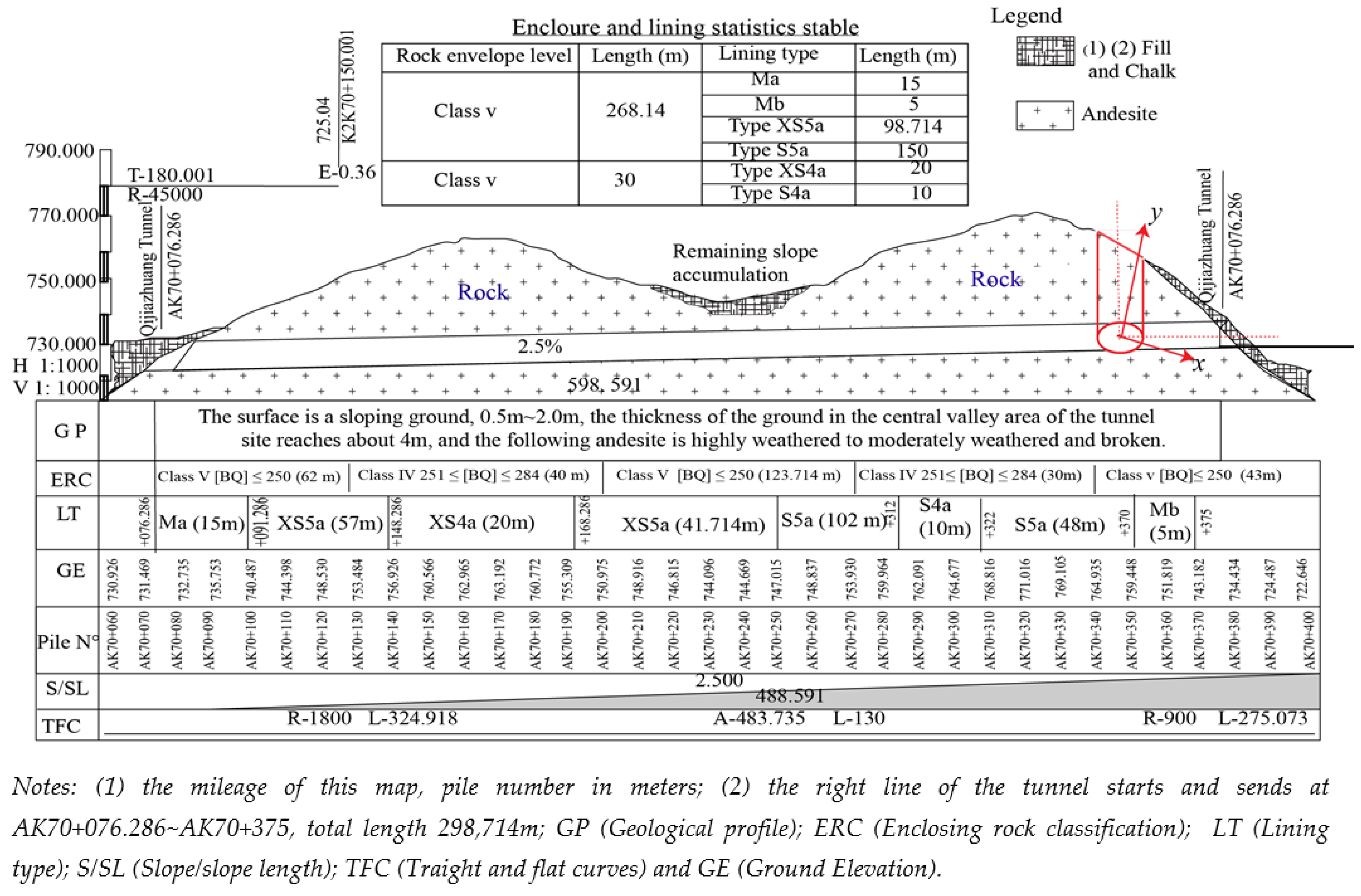
4.1. Presentation of Qijiazhuang Tunnel

This section uses geometric data from the Qijiazhuang tunnel in China to validate the analytically obtained results. Abaqus and Matlab are proposed to perform the numerical simulations. The input parameters are: $h_1$ = 55.03 m, $h_2$ = 6.69 m, $h$ = 19 m, $r$ = 5.9 m, $\beta$ = 27°, the diameter (D) = 11.861 m and the distance between $h_1$ and $h_2$ = 94.88 m. The annular radius $\alpha$ of the mapped $\varsigma -$ space is given by the value$\alpha =0.18$. As an excavation technique, the New Austrian tunnel method (NATM) is adopted. The mechanical parameters around the tunnel are presented in

Table 1. Mechanical parameter of the Qijiazhuang tunnel.

N°	Materials	E(GPa)	$\mathit{v}$	ϕ(°)	c(MPa)	${\mathit{\gamma }}_{\mathit{d}} (\mathbf{kN}/{\mathbf{m}}^3)$
1	soil	21 × 10-3	0.50	22	18 × 10-3	18
2	rock (highly weathered)	1.9	0.35	27	0.15	19
3	rock (moderately weathered)	1.95	0.35	29	0.25	19.5
4	rock (slightly weathered)	2.1	0.35	29	0.25	19.5
5	lining	35	0.25	—	—	25
6	Bolt and grout	11.0	0.25	30	1.35	20

E (GPa): modulus of deformation; $v$: Poisson ratios; ϕ(°): internal friction angle; c(MPa): cohesion; ${\gamma }_d$ (kN/m³) total soil weight.

.

4.2. Parametric Analysis of the Tunnel

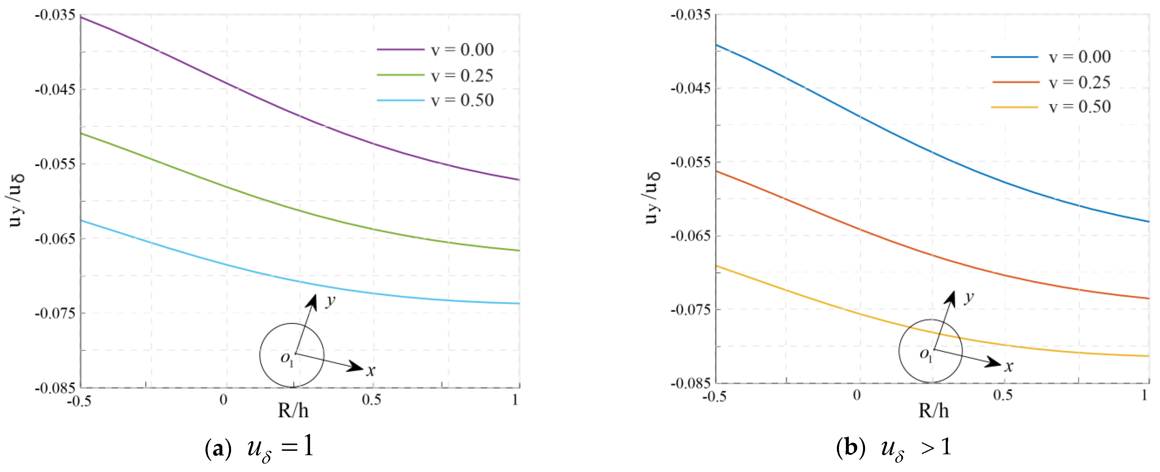
The effect of$\beta$,$R$,$h$, $h_1$, $h_2$, $u_0$, $u_{\delta }$ and $∆u_y$ on the deformation surface is presented in Figure 4.

4.2.1. Effect of $h$, $h_1$ and $h_2$

Vertical displacement due to unloading of the cavity is often influenced by the depth, or $p_0$< $p_1$. Figure 4 shows the effect of$h$, $h_1$ and $h_2$ on the tunnel wall. The input parameters are represented by$h$, $h_1$, $h_2$, $v$, R and $\alpha =0.18$.

The results of the planned vertical displacement show a settlement trough in the centre of the tunnel at the value $R/h$ = 0.5. This is due to the decrease in the unloading pressure. Following the direction of the slope inclination, the vertical displacement is influenced by the asymmetrical distribution of the surface load. The results of this approach make it possible to take into account the interaction between the load on the slope and the tunnel wall. Therefore, Figure 4 describes a good agreement between the predicted hypothesis and the results obtained.

4.2.2. Effect of Tunnel Radius

The stability of the tunnel is considerably affected by the radius and depth of the tunnel. When the tunnel radius increases, the maximum settlement on the ground surface becomes more evident, as shown in Figure 4. Then, when a tunnel is shallow, its width defines the type of deformation it can generate.

Figure 5 shows the basic displacement of the tunnel wall. Analytical operations reflect its modes. The changes in the deformation space $u_0$, $u_{\delta }$, $∆u_x$ and $∆u_y$ are variable, and the contour shape can be produced. The slight variations are small and can be accounted for [14]. The cross-sectional contour lines in Figure 5a,b are always symmetrical to$y$. Figure 5c,d illustrate the vertical and horizontal displacement, respectively, of the tunnel wall. As Verruijt and Strack [42] note, when the weight of gravity is greater than the weight of the structure, the tunnel moves upwards due to the “buoyancy effect”. The tunnel settles when the surface pressure is greater than the internal pressure. Therefore, the tunnel wall displacement tends to follow the direction of the slope.

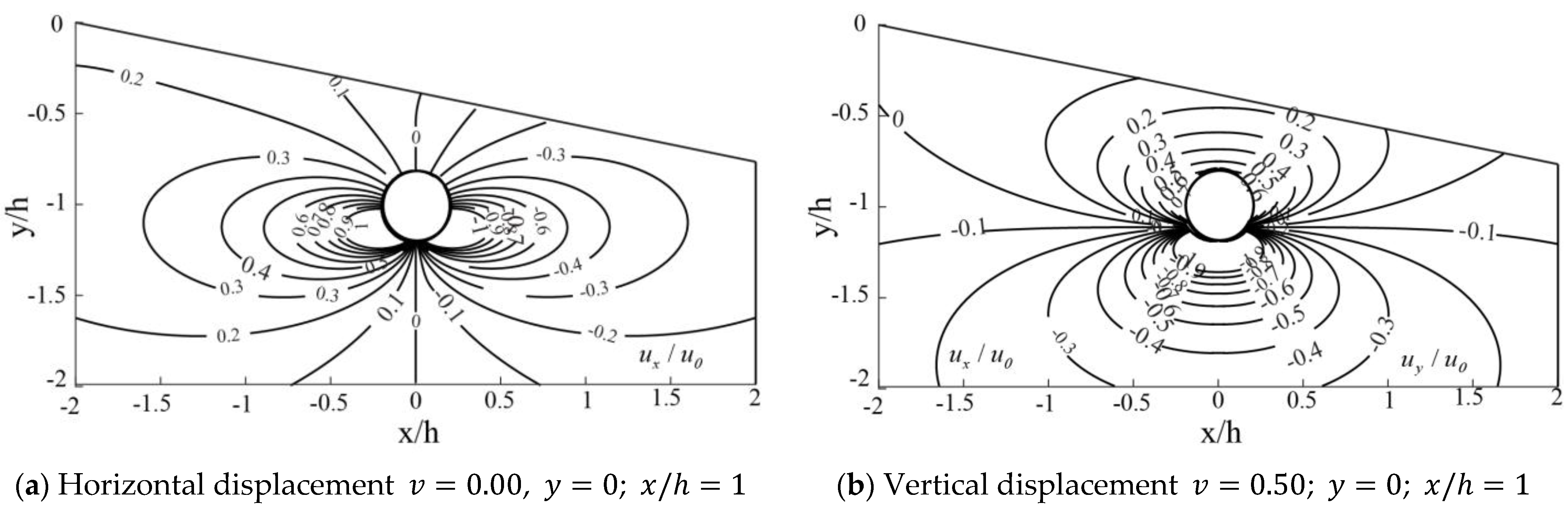
4.2.3. Effect of Contour Lines

The geometric parameters of the Figure 6, Figure 7, Figure 8 and Figure 9 are$h$ = 19 m, $h_1$ = 55.03 m, $h_2$ = 6.69 m $\beta$ = 27°, D = 11.861 m, E, v and ${\gamma }_d$. Figure 8 and Figure 9 summarize the stratigraphic displacement of the contour line to the tunnel wall around a shallow circular tunnel on the slope for the selected embedment ($R/h$) and the Poisson ratio $v$ = 0.25. In all cases, the vertical displacement is symmetric with respect to the$y-$ axis, while the horizontal displacement is asymmetric. The ground displacement distribution and their magnitude evaluated by means of the approximate solution on the slope do not depend on the $R/h$ ratio, since the displacement field is given by a function of the dimensionless coordinates $x/h$ and $y/h$ multiplied by $R/h$.

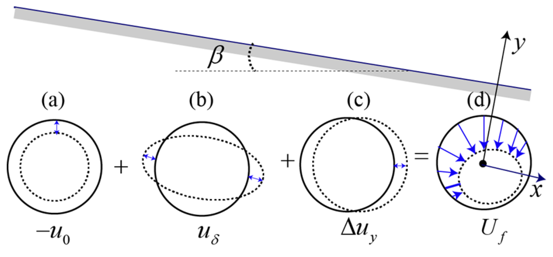
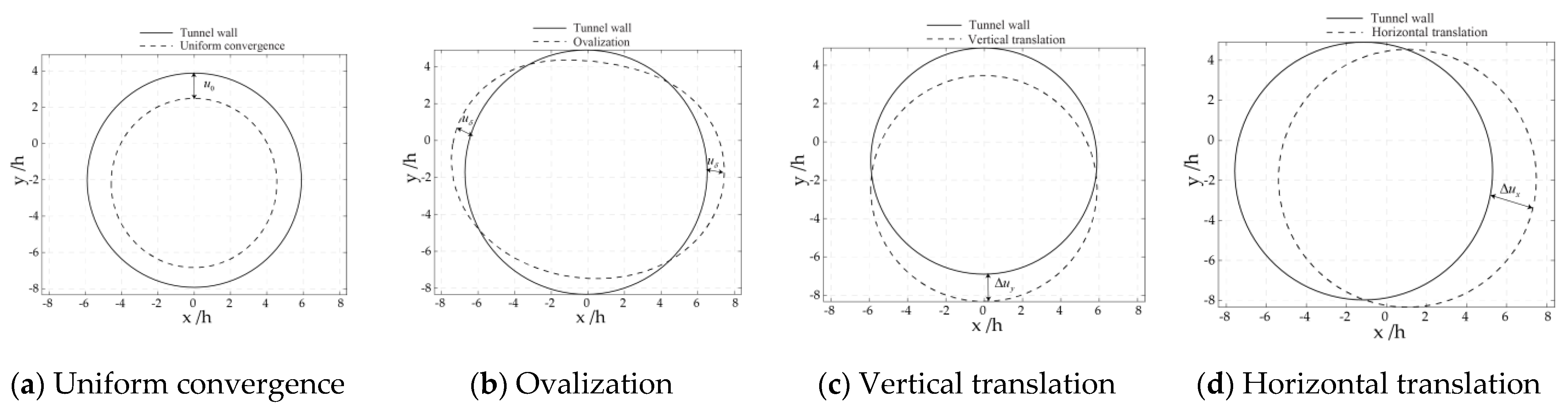
4.3. Analysis of the Deformation Parameters

4.3.1. Uniform Convergence

The uniform displacement shown in Figure 10, Figure 11 and Figure 12 illustrate the ground displacement as a function of$R/h$. The effect shown in Figure 12 represents the vertical translation as a function of $k$ numerated by Equations (36) and (37). The results highlight the importance of the Poisson ratio the smaller the translation correction. We note that the intercession point of these three figures has ordinates $R/h$ = 0; this implies that even when the ground surface is variable, the uniform convergence will undergo the same type of displacement by compression. Consequently, the ground loss around the tunnel will be uniform.

4.3.2. Ovalization Beneath the Slope

Figure 13 shows the values of the absolute of the maximum vertical motion induced by ovalization, the $u_x/u_{\delta }$ and $v$ values, where advantage has been taken of the fact that the horizontal displacement is asymmetric in $R/h$. It is noted that the maximum vertical displacement increases with the angle of the inclined plane. Deformed tunnels on the ground deformation induced by the slope for different Poisson ratios and $R/h$ are shown in Figure 13. Figure 14 shows the relationship between the horizontal and vertical displacement based on Equations (43)–(56). The input parameters are $\nu =0.50$, $y=0$, $x/h$ = 0 and $R/h$= 0.30. These approximate solutions are set at the two circular boundaries ($\left|\varsigma \right|=1$ and $\left|\varsigma \right|=\alpha$) of the mapped surface. The solutions are imposed by the “ovalization” of the tunnel. The horizontal displacement is symmetrical along the centre line and vertical to the tunnel axis. In contrast, the vertical displacement is asymmetrical to the centre line (coordinates (−2, −0.02) on the left and (2, −0.1) on the right). The vertical displacement is parallel to the slope surface. This specifies that the proposed analytical data accurately predict the direction of tunnel deformation when the ground surface is inclined. These same cases are also observed in Figure 15, which also follows the direction of the slope at the point $R/h=-0.3$. Using the parameters obtained in Equations (48) and (58), the ground displacement is evaluated by comparing the approximate solutions ($\left|\varsigma \right|=1$+$\left|\varsigma \right|=\alpha$ and $u_c$) and the exact solution (from Equations (25)–(31)). It can be seen that the reading of the curves is well reproduced, while the ground “rebound” trough given by the model is represented at $R/h=-0.3$ (Figure 15). Thus, as a function of the variation of the Poisson ratio, the curves are closer to each other. The approximate solution derived of the slope generates higher displacement at the tunnel crown, as can be seen in the deformation of the tunnel wall. This specifies that, regardless of the position of the slope angle, the results obtained can be a better prediction of the ground deformation around the tunnel. This shows that the comparison with the model prediction meets the criterion of slope stability.

As the ground surface induces an asymmetrical load on the tunnel wall, the actual ground motion is divided into two parts: the motion centered on the tunnel axis and the vertical translation. According to Wang et al. [31], the corresponding vertical translation could be upward or downward beneath a different focusing motion. Since the soil type at the depth of the Qijiazhuang tunnel is andesitic, the vertical translation shown in Figure 16 will not affect the soil loss because it is included in the vertical displacement.

Figure 17 shows the maximum vertical displacement induced by the slope. The settlement trough is asymmetrical to the tunnel axis at $R/h=-0.6$ (Figure 17a) and symmetrical in Figure 17b ($R/h=-0.65$). The curves vary with the Poisson ratio ($v$ = 0.00; 0.25; 0.50). The inclination of the maximum displacement follows the direction of the ground subsidence and the angle of the inclined plane. This displacement is established based on the stresses proposed in Section 3.1.

Loads are compared to the stresses inside the system (induced by the weight of the layers), with those obtained in situ, assuming that the tunnel wall is close to the ground surface. The results of the latter procedure, called “normal load approximation”, have been proposed in Section 3.1. The stresses in the vicinity of the tunnel cross-section are also obtained by the exact solution proposed in Section 3.1, assuming that the material at the base is a pair of very wide liners. Thus, the stresses applied to the tunnel wall will be symmetrical to the internal soil pressure.

The vertical and horizontal ground displacement is determined using the complex potential approach. Nevertheless, the ground displacement can be evaluated using any given reference point. The mechanical model is semi-infinite because the evaluation point of the deformation at infinity is considered a reference when the displacement of the left and right tunnel boundaries is at $u_0$. The Laurent series can then be generated in an annular domain. The point at infinity can thus be regarded as the non-moving reference, permitting the additional rigid body translation to compensate for the deficiency [27]. In a prior investigation, the displacement model based on symmetric stress redistributions along the $y-$ axis was developed by measuring the stresses on a plane surface [22]. This paper proposes the horizontal and vertical displacement of a rigid body due to the asymmetric stress distribution along the y-boundaries$\left|\varsigma \right|=1$ and $\left|\varsigma \right|=\alpha$. The tunnel wall is subjected to symmetrically distributed stresses. Several other factors that account for the ground deformation are considered. The horizontal and vertical displacement (Figure 18) generated by the slope can be defined by:

$$u_x+u_x\left(\left|\varsigma \right|=1\right)+u_x\left(\left|\varsigma \right|=\alpha \right)=-\frac{u_x\left(\left|\varsigma \right|=1\right)+u_x\left(\left|\varsigma \right|=\alpha \right)}{2}+u_x\left(\left|\varsigma \right|=1\right)+u_x\left(\left|\varsigma \right|=\alpha \right)=\frac{u_x\left(\left|\varsigma \right|=1\right)-u_x\left(\left|\varsigma \right|=\alpha \right)}{2}$$

(58)

For depth $h_1$ and $h_2$, we can have, respectively:

$$u_x|h_1=-\frac{u_x\left(\left|\varsigma \right|=1\right)-u_x\left(\left|\varsigma \right|=\alpha \right)+2u_x\left(\left|\varsigma \right|=1\right)}{2}$$

(59)

$$u_x|h_2=\frac{u_x\left(\left|\varsigma \right|=\alpha \right)-u_x\left(\left|\varsigma \right|=1\right)+2u_x\left(\left|\varsigma \right|=1\right)/\left(\left|\varsigma \right|=\alpha \right)}{2}$$

(60)

This is explained by the fact that the displacements determined in Equations (59) and (60) are established in equilibrium with $\left|u_x/h\right|\ne \left|u_x/h_1\right|\ne \left|u_x/h_2\right|$. The slope-induced asymmetric settlement effect is generally influenced by the variation in tunnel thickness. Based on $u_x$, $h_1$ and $h_2$, horizontal movement will not change the tunnel width when the tunnel is in equilibrium. In the same deformation mode, the vertical translation of the rigid body is strongly influenced by the “buoyancy” effect [1,20,42,43,44].

The rigid translational motion shown is influenced by the translation of the rigid materials. Considering the asymmetric compression from the upslope to the downslope, Strack and Verruijt [44] propose that the displacements are infinite at infinity due to the resultant force acting on the tunnel. Therefore, the frame of reference in this context is an unchanging point at infinity. Analyzing the asymmetric deformation generated by the slope, the load weight on the ground surface can be used to determine the vertical displacement.

4.4. Stress Evaluation around the Tunnel

To further investigate the ground deformation problem, the tunnel wall displacement field and the settlement trough are analyzed. For Figure 19, the deformations are established by the soil deformation factor (SDF), with $u_0$ = −0.002 m ($v_i$ = 0.6%). The contours of the vertical stress, horizontal stress, shear stress and maximum shear stress (for $\mathrm{y}=0$ and $\mathrm{x}=\pm \mathrm{h}$, ${\tau }_{xy}max=\pm 0.86u_0\mu \left(R/h\right)$) with the backfill and foundations are shown in Figure 19 with a tilt angle $\beta$ = 27°.

Figure 19 shows the direction of stress deformation as determined with SDF. The mesh displacements shown on SDF (1) and SDF (2) represent the direction of ground deformation. In order to obtain real values of the ground displacement, the settlement curves and the vertical displacement are evaluated on a numerical scale. At SDF (1), the surface-induced displacement exerts a compressive force on the central axis of the tunnel, while SDF (2) exerts a traction force that varies the tunnel radius. This variation is due to the ground deformation index, which varies between SDF (1) 1 and SDF (2) 15. When the tunnel is subjected to varying pressure, the tunnel radius tends to deform. Therefore, the ground displacement could be the product of the combined effect of the deformation mode of the tunnel section and “buoyancy” [20]. The figures show that the “normal loading approximation” considerably overestimates all the stresses and ground displacement around the tunnel.

The analysis presented in Section 4.3 shows that after the displacements represented from the Cartesian scale, the displacement curves sag considerably around the tunnel wall. This is due to the weathered nature of the rock (andesite) surrounding the tunnel. From the cross-section towards the centre of the tunnel, a uniaxial compressive strength can be estimated with laboratory experiments and geometric measurements of the rock burst, which in turn can be calibrated using the method proposed in this study in order to control the risk of “collapse” of the tunnel.

5. Application to Engineering Cases

The evaluation of the potential of the approximate method under a slope based on the complex potentials of the above Qijiazhuang tunnel predicts the ground displacement field. The field data of the section of National Highway 109 of the Sixth Western Bypass Section (SPO-SL) of the city is used for this analysis. The start and end of the straight line of the tunnel are from AK70+076286 to AK70+375, with a total length of 298.714 m (Figure 20). The tunnel is built beneath a slope with an angle of inclination of $\beta$ = 27°. The slope surface varies from 0.5 m to 2.0 m (Figure 20), and the thickness separating the central valley is about 4 m. The lithology is andesitic with three weathering phases (Table 1). The same process adopted for the mining excavation (New Austrian tunnel method: NATM) is used for the tunnel excavation, effectively controlling the ground deformation around the tunnel. Furthermore, grout injections are used to stabilize the rocks surrounding the tunnel. Although the stability measurement data on the ground surface is monitored, the complete ground displacement can only be analyzed with monitoring devices. However, with the approximate method under a slope proposed in this study, the parameters inducing the deformation of the tunnel wall (uniform convergence, ovalization, vertical and horizontal translation and shape of the final displacement) are determined.

The cross-section is used to predict the ground deformation around the tunnel (Figure 21). The resulting analytical data of the tunnel geometry is represented by ${ {\mathrm{A}}^{\prime } \mathrm{o}}_1={\mathrm{o}}_1 {\mathrm{B}}^{\prime }$ = 47.44 m, $h_1$= 55.03 m,$h_2$= 6.69 m and $R/h=0.31$. The ground deformation is analyzed taking into account the slope angle $\beta$ = 27°, E = 21 × 10⁻³ MPa, $v$ between 0.00 and 0.50, ${\gamma }_d$= 18$\mathrm{kN}/{\mathrm{m}}^3$, the slope of the tunnel longitudinal axis 2.5% and $u_0$= −0.04 m ($v_i$ = 0.6%). These geometric and in situ data were used to digitize Figure 21. The same data were also used to build the model shown in Figure 22, which presents a comparative pattern between the analytical solution and the numerical simulation. The difference in vertical displacement is due to the angle of the inclined plane, which gives it an asymmetric displacement on the negative image pole ($y=h$). Thus, due to the asymmetric stress distribution, the load applied in the numerical simulation is influenced by the nature of the weathered material, hence the presence of an asymmetry in the negative part of Figure 22.

When Equation (3) is used as the exact boundary condition in the tunnel cross-section, the approximate method beneath a slope obtained in Equations (39), (48) and (58) is used to model and justify the results given by the exact solution considering the asymmetric compression. A degree of rationality is always necessary in defining a design analysis, and it is essential that the design engineer is able to assess the overall accuracy of a numerical analysis as far as possible [41]. These values must be defined by determining the thickness of each soil layer level on the tunnel roof. At this stage, Mitchell still needed to present the complete solution for the elastic stresses and displacements around a doubly symmetric tunnel. Thus, the effect of internal pressure alone cannot change the tunnel equilibrium. It would be necessary for the two pressures $p_0$ and $p_1$ to interact on the tunnel, equilibrating the pressure of the excavation trough under the effect of the stress gradient.

Moreover, the equilibrium equations and the geometric application of the tunnel are known (in an elastic plane). In this way, Kong et al. [15] estimate that the boundary condition of the tunnel cross-section displacement can be easily realized on a real project. Thus, considering the geometry of the Qijiazhuang tunnel, the complex variable method also solves the problem of the lithological variation surrounding the tunnel. Consequently, taking into account the surface slope and the variable soil thickness, the accelerated weathering of the andesite can be controlled by the confining pressure calculated based on the progressive rock movement. As the central valley of the site is overflowing with water, a fluid transfer method could redirect the “seepage” out of the tunnel. Depending on the results obtained, the complex analytical function can be the best way to predict the ground deformation around a tunnel beneath a slope.

6. Conclusions

The deformation of a tunnel under a slope is usually caused by the asymmetric stress distribution over the tunnel cross-section. Fourier series expansion is used to determine the contour line surrounding the tunnel. This study proposes an approximate solution beneath the slope for predicting the ground deformation around the tunnel. The analytical method of ground displacement is proposed by the complex potential method, obtained by using the elastic problem in a circular domain.

A definition of the exact and approximate solutions beneath the tunnel is given. The mathematical derivations and integrations for modelling the ground displacements due to the tunnel excavation under an inclined plane are based on continuum mechanics. The soil model resulting from the deformation is studied, and the factors influencing the stress distribution in the soil are identified and redefined in a simple soil compression form. A definition of the exact and approximate solutions under the slope for the maximum soil displacement is established. Conformal convergence, ovalization and vertical translation establish control parameters for the displacement distribution. It is found that both solutions give similar results. This implies that the control factors for the ground displacement parameters are established based on the presence of the internal friction angle and the slope-induced friction force. The effect of tunnel geometry was also proposed to calculate the weight of the load on the ground surface. The results show that the effect of the geometry has more influence on the direction of the downslope because the contact between the ground surface and the tunnel wall is small.

To verify the analytical solutions numerically, a series of numerical simulations for different deformation modes are proposed. The analysis of the parameters shows that the model used for the cross-section has considerable effects on the behavior of the displacement field below the slope limit. Furthermore, the ground behavior at the cross-section can determine the ground movement around the tunnel and the surface settlement by equilibrating the stresses at the boundary conditions. The deformation type is also influenced by the tunnel geometry and the angle of the inclined plane.

Data from the Qijiazhuang tunnel in China were used for numerical modelling of the tunnel cross-section. Keeping in mind that the continuum theory would work perfectly with the asymmetric stress distribution, the complex potential and displacement theory is proposed, which is a second-order justification in the classical ground deformation theory, to take into account the stress variation and the downslope proximity effect. It is argued that these prediction-based theories exhibit a conjunction with the basic criterion of maximum displacement, even when the angle of the inclined plane is variable. Thus, with this approach, the results show that the proposed analytical method is compatible with the quantitative data of the Qijiazhuang tunnel. This indicates that the analytical solutions could be an excellent alternative model for tunnel deformation risk assessment. The proposed method can also predict inelastic ground deformation in preliminary tunnel studies.

References

1. Fu, J.; Yang, J.; Klapperich, H.; Wang, S. Analytical Prediction of Ground Movements due to a Nonuniform Deforming Tunnel. Int. J. Geomech. 2015, 16, 04015089. [Google Scholar] [CrossRef]
2. Peck, R.B. Deep excavations and tunneling in soft ground. In Sociedad Mexicana de Mecanica, Proceedings of the 7th International Conference on Soil Mechanics and Foundation Engineering, Mexico City; International Society for Soil Mechanics and Geotechnical Engineering: London, UK, 1969; pp. 225–290. [Google Scholar]
3. Mair, R.J.; Taylor, R.N.; Bracegirdle, A. Subsurface settlement profiles above tunnels in clays. Geotechnique 1993, 43, 315–320. [Google Scholar] [CrossRef]
4. O’Reilly, M.P.; New, B.M. Settlements above tunnels in the United Kingdom—Their magnitude and prediction. PT 82 IMM. London 1982, 20005, 173–181. [Google Scholar] [CrossRef]
5. Dyer, M.R.; Hutchinson, M.T.; Evans, N. Symposium on Geotechnical Aspects of Underground Constructions in Soft Ground Sudden Valley Sewer: A case history. In Proceedings—International London; Balkema: Rotterdam, The Netherland, 1996; pp. 671–676. [Google Scholar]
6. Moh, Z.C.; Hwang, R.N.; Ju, D.H. Ground movements around tunnels in soft ground. In Geotechnical Aspects of Underground Construction in Soft Ground; Elshafie, M., Viggiani, G., Mair, R., Eds.; Balkema: Rotterdam, The Netherland, 1996; pp. 725–730. [Google Scholar]
7. Wei, G.; Pang, S.; Zhang, S. Prediction of ground deformation induced by double parallel shield tunneling. Disaster Adv. 2013, 6, 91–98. [Google Scholar]
8. Pinto, F.; Zymnis, D.M.; Whittle, A.J. Ground Movements due to Shallow Tunnels in Soft Ground. II: Analytical Interpretation and Prediction. J. Geotech. Geoenviron. Eng. 2014, 140, 04013041. [Google Scholar] [CrossRef] [Green Version]
9. Amorosi, A.; Boldini, D.; De Felice, G.; Malena, M.; Sebastianelli, M. Tunneling-induced deformation and damage on historical masonry structures. Geotechnique 2014, 64, 118–130. [Google Scholar] [CrossRef]
10. Hasanpour, R. Advance numerical simulation of tunneling by using a double shield TBM. Comput. Geotech. 2014, 57, 37–52. [Google Scholar] [CrossRef]
11. Zheng, G.; Lu, P.; Diao, Y. Advance speed-based parametric study of greenfield deformation induced by EPBM tunneling in soft ground. Comput. Geotech. 2015, 65, 220–232. [Google Scholar] [CrossRef]
12. Zheng, G.; Zhang, T.; Diao, Y. Mechanism and countermeasures of preceding tunnel distortion induced by succeeding EPBS tunneling in close proximity. Comput. Geotech. 2015, 66, 53–65. [Google Scholar] [CrossRef]
13. Zhang, Z.; Huang, M.; Zhang, M. Theoretical prediction of ground movements induced by tunnelling in multi-layered soils. Tunn. Undergr. Space Technol. 2011, 26, 345–355. [Google Scholar] [CrossRef]
14. Zhang, Z.G.; Huang, M.S.; Xi, X.G.; Yuan, X. Complex variable solutions for soil and liner deformation due to tunneling in clays. Int. J. Geomech. 2018, 18, 0001197. [Google Scholar] [CrossRef]
15. Kong, F.; Lu, D.; Du, X.; Shen, C. Displacement analytical prediction of shallow tunnel based on unified displacement function under slope boundary. Int. J. Numer. Anal. Methods Geomech. 2018, 2018, 183–211. [Google Scholar] [CrossRef] [Green Version]
16. Mindlin, R.D. Stress distribution around a tunnel. Trans. Am. Soc. Civil Eng. 1940, 195, 1117–1140. [Google Scholar] [CrossRef]
17. Zymnis, D.M.; Whittle, A.J.; Chatzigiannelis, I. Effect of anisotropy in ground movements caused by tunneling. Geotechnique 2013, 63, 1083–1102. [Google Scholar] [CrossRef] [Green Version]
18. Fang, Q.; Song, H.R.; Zhang, D.L. Complex variable analysis for stress distribution of an underwater tunnel in an elastic half plane. Int. J. Numer. Anal. Methods Geomech. 2015, 39, 1821–1835. [Google Scholar] [CrossRef]
19. Lu, A.Z.; Zeng, X.T.; Xu, Z. Solution for a circular cavity in an elastic half plane under gravity and arbitrary lateral stress. Int. J. Rock Mech. Min. Sci. 2016, 89, 34–42. [Google Scholar] [CrossRef]
20. Lu, D.; Kong, F.; Du, X.; Shen, C.; Gong, Q.; Li, P. A unified displacement function to analytically predict ground deformation of shallow tunnel. Tunn. Undergr. Space Technol. 2019, 88, 129–143. [Google Scholar] [CrossRef]
21. Wang, H.N.; Wu, L.; Jiang, M.J.; Song, F. Analytical stress and displacement due to twin tunneling in an elastic semi-infinite ground subjected to surcharge loads. Int. J. Numer. Anal. Methods Geomech. 2018, 42, 809–828. [Google Scholar] [CrossRef]
22. Mabe Fogang, P.; Liu, Y.; Zhao J, l.; Azeuda Ndonfack, K.I. Soil Deformation around a Cylindrical Cavity under Drained Conditions: Theoretical Analysis. Adv. Civ. Eng. 2022, 2022, 4127660. [Google Scholar] [CrossRef]
23. Yang, G.; Zhang, C.; Min, B.; Chen, W. Complex variable solution for tunneling-induced ground deformation considering the gravity effect and a cavern in the strata. Comput. Geotech. 2021, 135, 104154. [Google Scholar] [CrossRef]
24. Mindlin, R.D. Stress distribution around a hole near the edge of a plate under tension. PSESA 1948, 5, 56–68. [Google Scholar]
25. Sagaseta, C. Analysis of undrained soil deformation due to ground loss. Geotechnique 1987, 37, 301–320. [Google Scholar] [CrossRef]
26. Verruijt, A.; Booker, J.R. Surface Settlements Due to Deformation of A Tunnel in an Elastic Half Plane. Geotechnique 1996, 46, 753–756. [Google Scholar] [CrossRef]
27. Verruijt, A. A complex variable solution for a deforming circular tunnel in an elastic half-plane. Int. J. Numer. Anal. Methods Geomech. 1997, 21, 77–89. [Google Scholar] [CrossRef]
28. Loganathan, N.; Poulos, H.G. Analytical Prediction for Tunneling-Induced Ground Movements in Clays. J. Geotech. Geoenviron. Eng. 1998, 124, 846–856. [Google Scholar] [CrossRef]
29. Verruijt, A. Deformations of an elastic half plane with a circular cavity. Int. J. Solids Struct. 1998, 35, 2795–2804. [Google Scholar] [CrossRef]
30. Massinas, S.A.; Sakellariou, M.G. Closed-form solution for plastic zone formation around a circular tunnel in half-space obeying Mohr-Coulomb criterion. Geotechnique 2009, 59, 691–701. [Google Scholar] [CrossRef]
31. Wang, L.-Z.; Li, L.-L.; Lv, X.-J. Complex Variable Solutions for Tunneling-Induced Ground Movement. Int. J. Geomech. 2009, 9, 63–72. [Google Scholar] [CrossRef]
32. Boussinesq, J. Essai Sur La Théorie Des Eaux Courantes; Institut National de France: Paris, France, 1877. [Google Scholar]
33. Jong, Y.G.; Liu, Y.; Zixuan Chen, Z.; Mabe Fogang, P. Hypoplastic Interface Model considering Plane Strain Condition and Surface Roughness. Adv. Civ. Eng. 2021, 2021, 1473181. [Google Scholar] [CrossRef]
34. Lee, K.M.; Rowe, R.K.; Lo, K.Y. Subsidence owing to tunnelling. I. Estimating the gap parameter. Can. Geotech. J. 1992, 29, 929–940. [Google Scholar] [CrossRef]
35. Gonzalez, C.; Sagaseta, C. Patterns of soil deformations around tunnels. Application to the extension of Madrid Metro. Comput. Geotech. 2001, 28, 445–468. [Google Scholar] [CrossRef]
36. Park, K.H. Elastic solution for tunneling-induced ground movement in clays. Int. J. Geomech. 2004, 310–318. [Google Scholar] [CrossRef]
37. Park, K.H. Analytical solution for tunnelling-induced ground movement in clays. Tunn. Undergr. Space Technol. 2005, 20, 249–261. [Google Scholar] [CrossRef]
38. Vasiliev, V.V.; Lurie, S.A.; Salov, V.A. On the Flamant problem for a half-plane loaded with a concentrated force. Acta Mech. 2021, 232, 1761–1771. [Google Scholar] [CrossRef]
39. Muskhelishvili, N.I. Some Basic Problems of the Mathematical Theory of Elasticity; P. Noordhoff Ltd.: Groningen, The Netherlands, 1963. [Google Scholar]
40. Mitchell, L.H. Stress-concentration factors at a doubly-symmetric hole. Aeronaut. Quart. 1966, 17, 177–186. [Google Scholar] [CrossRef]
41. Exadaktylos, G.E.; Liolios, P.A.; Stavropoulou, M.C. A semi-analytical elastic stress–displacement solution for notched circular openings in rocks. Int. J. Solids Struct. 2003, 40, 1165–1187. [Google Scholar] [CrossRef]
42. Verruijt, A.; Strack, O.E. Buoyancy of tunnels in soft soils. Geotechnique 2008, 58, 513–515. [Google Scholar] [CrossRef]
43. Fu, J.Y.; Yang, J.S.; Yan, L.; Abbas, S.M. An analytical solution for deforming twin-parallel tunnels in an elastic half plane. Int. J. Numer. Anal. Methods Geomech. 2015, 39, 524–538. [Google Scholar] [CrossRef]
44. Strack, O.E.; Verruijt, A. A complex variable solution for a deforming buoyant tunnel in a heavy elastic half-plane. Int. J. Numer. Anal. Methods Geomech. 2022, 26, 1235–1252. [Google Scholar] [CrossRef]
Figure 1. Geometrical representation of a shallow tunnel model beneath an inclined plane.
Applsci 13 03252 g001
Figure 2. Basic displacement of the tunnel wall.
Applsci 13 03252 g002
Figure 3. Conformal mapping of a tunnel beneath an inclined plane.
Applsci 13 03252 g003
Figure 4. Effect of h , h 1 , and h 2 on tunnel wall.
Applsci 13 03252 g004
Figure 5. Basic displacement of the tunnel wall.
Applsci 13 03252 g005
Figure 6. Stratigraphic displacement of the tunnel wall (uniform convergence).
Applsci 13 03252 g006
Figure 7. Displacement induced by uniform convergence.
Applsci 13 03252 g007
Figure 8. Displacement induced by ovalization.
Applsci 13 03252 g008
Figure 9. Displacement induced by Equations (33)–(35) (uniform convergence) and Equations (50)–(56) (ovalization).
Applsci 13 03252 g009
Figure 10. Vertical translation of the tunnel wall.
Applsci 13 03252 g010
Figure 11. Superposition of vertical translation and vertical ground motion.
Applsci 13 03252 g011
Figure 12. Effect of vertical translation affected by k.
Applsci 13 03252 g012
Figure 13. Maximum vertical displacement.
Applsci 13 03252 g013
Figure 14. Approximate solution on the slope for R / h = 0.5, x / h = 0   v = 0.50 , −0.09 < u x < 0.09.
Applsci 13 03252 g014
Figure 15. Relationship between the approximate solution on the slope and the exact solution.
Applsci 13 03252 g015
Figure 16. Vertical translation.
Applsci 13 03252 g016
Figure 17. Vertical displacement.
Applsci 13 03252 g017
Figure 18. Horizontal and vertical displacement given by ovalization.
Applsci 13 03252 g018
Figure 19. Tunnel deformation beneath an inclined plane.
Applsci 13 03252 g019
Figure 20. 2–4 longitudinal section of Qijiazhuang Tunnel (S4a).
Applsci 13 03252 g020
Figure 21. Numerical representation of the meshes around a tunnel beneath an inclined plane.
Applsci 13 03252 g021
Figure 22. Comparative analysis between the analytical solution and the numerical simulation.
Applsci 13 03252 g022