1. Introduction
In recent years, computer vision has become increasingly mature, with the successful development of artificial intelligence technology and a dramatic increase in the computing power of hardware devices. A more fundamental task in this field, human pose estimation, is gradually becoming a hot topic. Thanks to the development of video capture devices and networks, it is essential to analyze and understand human posture from video data or image data [
1] and then prepare it for tasks such as motion recognition, anomaly detection, autonomous driving, and human–computer interactions.
The essence of human pose estimation is to detect the essential parts and major joints of the human body in the video or picture, such as the eyes, nose, hands, shoulders, knees, feet, etc. It generally includes single-person scene detection and multi-person scene detection, the former of which is relatively simple and only requires the algorithm to extract the feature points of body parts and create a connected pose. In contrast, multi-person scene detection is more complex, mainly consisting of “top-down” and “bottom-up” methods. “Top-down” refers to identifying all the bodies in the video or picture first, followed by identifying the feature points of each person. The “bottom-up” approach first identifies all the feature points in the video or image [
2] and then corresponds all the feature points to the relative human body through an algorithm.
In this paper, we take the application scenario of human pose estimation, i.e., an anomaly detection task, as there is no fixed basis for determining “abnormal human behavior”. For example, actions occurring at different positions in a fixed scene, actions occurring at different moments in a fixed scene, and different actions occurring at the same position and at the same moment in a specific scene can be judged as “abnormal behavior”. This is because whether human or an animal, behavior often depends on posture, movement, and the environment. For example, drawing on a blackboard is normal behavior, while drawing on a monument is judged as “abnormal”.
In addition, the lower probability of abnormal behavior compared to normal behavior makes data acquisition more difficult, which leads to an imbalance of positive and negative samples and makes it difficult for the model to learn enough features of abnormal behavior. In addition, the model performance is limited by the lighting, angle, and object movement speed [
3]. Most detection methods also face the problems of complex behavior recognition, a multi-parameter search space, and high computational cost [
4]. This is due to the differences in the appearance of the human body and the need to ensure multiple targets associated with time sequence are not skipped or missed when detecting different behaviors in video or image data, which leads to a sharp increase in the algorithm parameters and computation, making the training process increasingly complicated and ultimately reducing the performance of the model.
For example, the supervised convolutional neural network proposed by Newell et al. [
5] to accomplish detection and grouping tasks can perform pose estimation in multi-person scenes. The AlphaPose [
6] algorithm proposed by Shanghai Jiao Tong University can perform self-body estimation tasks while ensuring a balanced real-time performance and pose estimation accuracy. Park et al. [
7] used convolutional neural networks to connect 2D pose results with image features for end-to-end learning to solve 3D human pose estimation tasks.
In addition, the human behavior detection algorithm proposed by Satybaldina [
8] to detect the front of ATMs based on gesture features has poor model performance due to the influence of the surrounding environment, such as pedestrians, fallen leaves, and lighting. Although the algorithm proposed by Chengfei [
9] to estimate the human posture of students in schools has improved significantly in model performance, it has many parameters and the model training process is complicated. The DNN model proposed by Toshev et al. [
10] uses the AlexNet network to capture different joint features; however, the weight parameters obtained by this method are more coupled with the training data distribution.
In contrast, graph convolutional networks are more adept at handling typical non-Euclidean structured data such as human skeleton information. For example, the ST-GCN algorithm based on human skeleton joints proposed by Yan [
11] combines a graph convolutional network (GCN) [
12] and a temporal convolutional network (TCN) [
13]. It extends to the spatial-temporal graph model, which forms a hierarchical representation of the skeleton sequence through a spatial-temporal graph. The GCN module is used to learn the local features of adjacent joints in space, and the TCN module is used to learn the local features of joint changes with time.
The space-time-separable graph convolutional network (STS-GCN) proposed by Sofianos et al. [
14] includes the temporal evolution and the spatial joint interaction within a single-graph framework, which favors the cross-talk of space and time, while bottlenecking the space-time interaction allows to better learn the fully-trainable joint and time interactions. A novel graph-based method was proposed by Y. Cai et al. [
15] to tackle the problem of 3D human body and 3D hand pose estimation from a short sequence of 2D joint detections. The method first uses a pre-trained cascaded pyramid network [
16] for 2D pose prediction and then feeds it into a spatial temporal graph convolution network. The spatial temporal graph convolution connects each joint to its corresponding joint in adjacent frames in the time dimension and connects the joint points in each frame that have direct and indirect kinematic dependencies (adjacent and symmetric) in the spatial dimension. The joints are also classified into six classes, and different convolution kernels are used for training for different node classes.
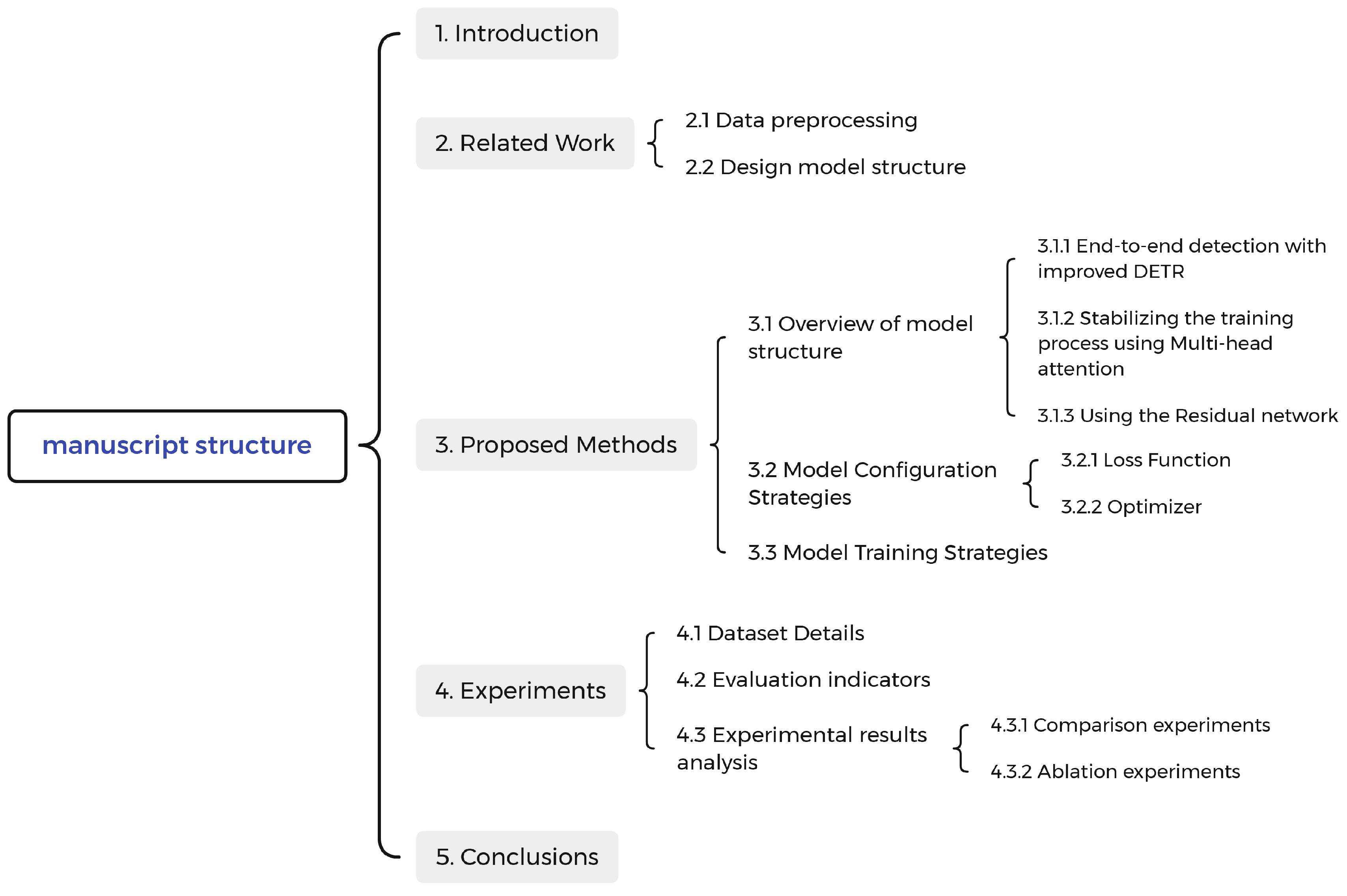
The manuscript structure is shown in
Figure 1 and the rest of this paper is organized as follows. In
Section 2, we introduce the work related to data preprocessing and model structure design. In
Section 3, we introduce the improved algorithm in detail including the model structure, the model configuration strategy, and the model training strategy.
Section 4 is the experimental part, including an introduction to the dataset used in the improved algorithm, model evaluation indicators, comparison experiments, ablation experiments, and experimental results analysis. Furthermore, finally, we conclude the paper in
Section 5.
3. Proposed Methods
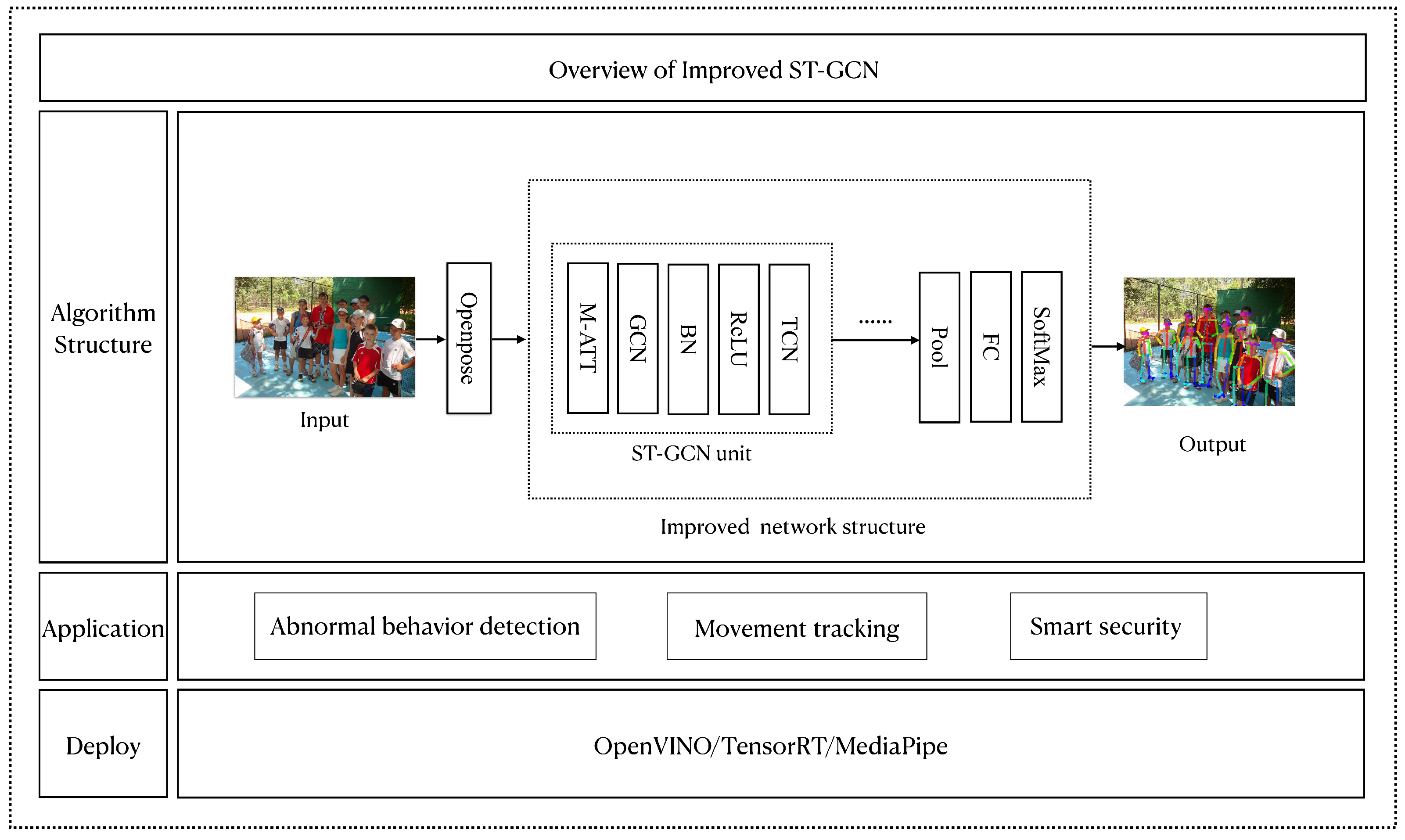
The flowchart of this algorithm is shown in
Figure 5, the general flow is as follows. Firstly, the skeletal points are extracted frame by frame from the dataset used in this paper by the OpenPose algorithm, and the skeletal points are used as the pre-input of the improved ST-GCN network. Then, the temporal and spatial dimensions are transformed by the ST-GCN unit, and the TCN and GCN modules are used alternately to transform the joint features. It is worth noting that this algorithm also introduces the multi-headed attention mechanism and residual network and redesigns the transformer DETR structure. Finally, after processing the ST-GCN unit, the output results go through the average pooling layer, the fully connected layer and finally the softmax to complete the output.
3.1. Overview of Model Structure
The network structure of the improved ST-GCN is shown in
Figure 6, and its core idea contains the following three aspects. Firstly, in terms of the network model structure, the improved network model still maintains the original ST-GCN nine-layer structure. The TCN module is used alternately with the GCN module with the following differences: Firstly, an improved DETR structure is added, i.e., the OpenPose algorithm module is used to complete skeletal point extraction frame by frame and replace the previous CNN module, which can detect all objects in parallel and avoid the generation of NMS and anchor points. Secondly, the improved network changes the attention model before the graph convolution operation to M-ATT and adds batch normalization (BN) [
29] and rectified linear units (ReLU) [
30] between the GCN module and the TCN module. The structure of the first eight ST-GCN units remains the same. Thirdly, a 9th ST-GCN unit is introduced into the residual network. From the training strategies, the expressiveness, detection performance, and generalization ability of the model are significantly improved by using warmup [
31], stepwise-cosine, mix-up [
32], and regularization strategies.
3.1.1. End-to-End Detection with an Improved DETR
Most detection methods perform detection based on detectors such as an anchor or Dense Box. However, since these methods perform repeated detection of the same target body, i.e., redundant detection frames are predicted, this problem must be addressed by means such as NMS. In contrast, the DETR structure proposed by Carion et al. does not require prediction of a candidate anchor and directly uses the model for violent regression.
Therefore, this method combines DETR and improves it. The whole DETR architecture consists of extracting skeletal points frame by frame by the OpenPose algorithm and encoder-decoder architecture, which does not require any custom network structure and simplifies the training process. It only requires a fixed set of object queries (query object); the DETR will predict the results in parallel based on the relationship between the target object and the global image context. The structure of the improved DETR is shown in
Figure 7.
The input data will first be extracted by the OpenPose algorithm frame by frame and then combined with positional encoding as the input data of the encoder. The decoder will use a small number of fixed query objects and the encoder output as the input of the decoder at the same time. The decoder-processed data will flow into the improved ST-GCN-1 unit and be used as the input of the improved ST-GCN network. In the original ST-GCN network, which contains nine layers, the GCN and TCN modules are used alternately to transform the temporal and spatial dimensions. In the GCN module, a random division is used to combine the graph convolution operations of three subgraphs into one, which effectively improves the computational performance of the algorithm.
The DETR uses a decoder to predict a fixed number of detection frames; it does not need to use post-processing means such as NMS. It uses the set loss function as a supervised signal for end-to-end training, where the set loss function uses the bipartite matching algorithm to match the prediction object with the ground truth object, as shown in Equation (
2):
where
y denotes the ground truth target set,
denotes the
N elements in the prediction set, and
denotes the loss value of the prediction and ground truth matching about element i of
. The matching effect is shown in
Figure 8.
Figure 8 contains the correspondence between two sets of prediction and ground truth, each set contains
N target bodies, and each target body contains two elements, which are the confidence level of the class to which the target body belongs (
, where
) and the location and size of the target body (
, where
, containing the center point of location coordinates and the width and height of the detection box). After matching the elements in the two sets, for example, (
) in the prediction sets corresponds to (
) in the ground truth, etc. (where ⌀ indicates that the class is empty), the Hungarian algorithm can be used to calculate its loss value, which abstracts the target detection task as a set prediction problem and then predicts all targets simultaneously and trains them end-to-end by set loss, thus simplifying the model training process and effectively avoiding problems such as anchor and NMS.
3.1.2. Stabilizing the Training Process Using Multi-Head Attention
The original ST-GCN network is designed with a layer of attention model to weigh the human torso before the graph convolution operation on the data. In contrast, M-ATT is introduced in the improved ST-GCN proposed in this paper, which can ensure that the DETR notices the information of different subspaces, which is beneficial for the network to capture richer feature information. It uses GCN and TCN alternately to transform the temporal and spatial dimensions, up-dimensionalize the human joint feature dimension, and down-dimensionalize the key frame dimension. Finally, the output result of the improved ST-GCN unit is output after the average pooling layer, the fully connected layer, and SoftMax, as shown in
Figure 9, which is the M-ATT structure diagram.
Each head in M-ATT contains its parameters, and the integration of each M-ATT output is as follows: ST-GCN-1 to ST-GCN-8 are integrated by “splicing”, and ST-GCN-9 is integrated by “averaging”. When given
,
, and
, each attention
is calculated as shown in Equation (
3):
where
f denotes a function of convergent attention and
,
, and
are learnable parameters.
Next, the results of each attention are stitched together and subjected to a linear transformation to obtain the final result, as shown in Equation (
4).
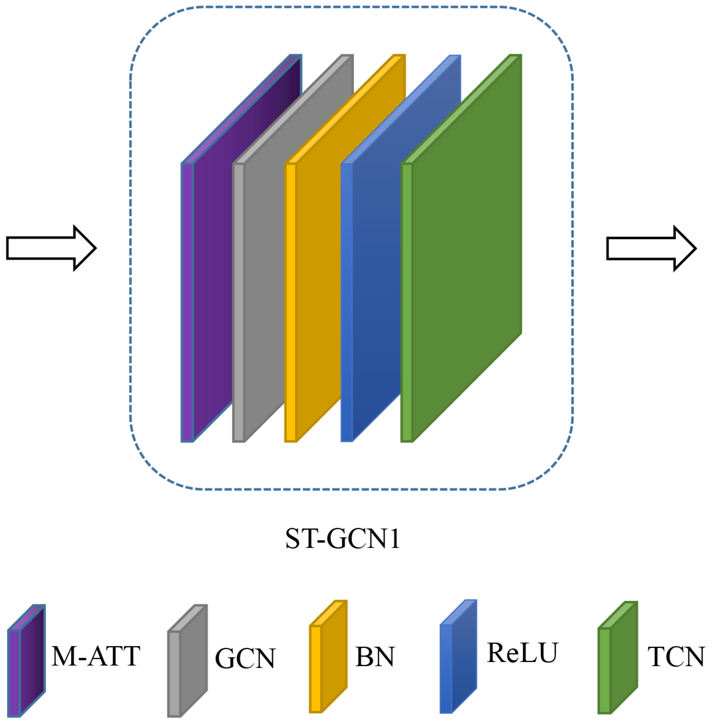
The application of M-ATT in improved ST-GCN is shown in
Figure 10 (
Figure 10 shows the ST-GCN-1 unit).
3.1.3. Using the Residual Network
Each cell of the original ST-GCN network will have a residual module and use dropouts for feature processing to enhance the spatial temporal information. This method is based on the structure of the original ST-GCN network. It adds a residual network in the ninth cell, which is used to solve the phenomenon of network degradation in deep networks and improve the model’s accuracy, as shown in Equation (
5), which is the primary representation of a residual block.
where
denotes the direct mapping, which is defined in Equation (
6).
in Equation (
6) denotes the 1*1 convolution operation and
is the residual part, as shown in
Figure 11 (a structure diagram of the residual network designed in this method).
3.2. Model Configuration Strategies
3.2.1. Loss Function
In the selection of the loss function, this paper combines the characteristics of the pose estimation task, assuming that the set of real poses of a human body is
, where the parameter
n is the batch size. The anchor pose is denoted as
, where the parameter
m indicates the number of anchor poses. The set of anchor pose labels is
, the set of output results corresponding to the regression branch is
, the set of output results corresponding to the classification branch is
, and the value corresponding to the regression amount is the difference between the true pose and the corresponding anchor pose
. The loss function of the regression branch adopts the mean square error loss
, and the classification loss adopts the cross entropy loss
, where
denotes the output value corresponding to the
ith data regression branch,
denotes the regression volume of the
ith data,
indicates the label value of the
i th data anchor pose, and
indicates the probability that the output of the classification branch of the
ith data belongs to the
jth anchor pose, as shown in Equation (
7), which is the loss function used in this model.
Among these metrics, the likelihood function of the regression branch obeys a Gaussian distribution with a mean value of the regression branch output and variance of , where is a learnable parameter. In the process of model inference, the output result of the regression branch is used as the final output result of , where denotes the output result of the regression branch and denotes the anchor pose corresponding to the input data.
3.2.2. Optimizer
When choosing an optimizer, the momentum-based SGD [
33] algorithm is used in this paper instead of the original SGD algorithm because the update direction of the original SGD algorithm entirely depends on the gradient calculated by the current batch, which in turn leads to a less stable model. In contrast, the momentum-based SGD algorithm simulates the inertia of an object in motion by borrowing the concept of momentum from physics, preserves the direction of the previous update to some extent during the update, and fine-tunes the final update direction using the gradient of the current batch, i.e., replaces the real gradient with the momentum before accumulation.
The SGD algorithm based on momentum observes the historical gradient. It reduces the gradient in the current direction if the current gradient is not consistent with the historical gradient direction; conversely, if the current gradient is consistent with the historical gradient direction, the gradient in the current direction is increased. In general, at the beginning of model iteration, the current gradient of the model is consistent with the direction of the historical gradient, so momentum will play an important role in helping the model reach the optimal point more quickly. In contrast, at the later stage of model iterations, the model’s current gradient is inconsistent with the direction of the historical gradient. It oscillates around the convergence value, so momentum will play a decelerating role in increasing the stability of the model and thus stop the model from falling into a local optimum.
Assuming that SGD depends on the gradient of the current batch, the current gradient,
, is calculated as shown in Equation (
8), where
denotes the gradient and
denotes the learning rate.
where
is the momentum factor. In addition to this, the warmup strategy is also used as the method of learning the rate decay. The variation in learning rate with epoch value is shown in
Figure 12. It can be observed that the learning rate gradually increases at the early stage of network model training, i.e., when
, when the model will correct the data distribution, which helps to slow down the overfitting phenomenon that may occur in the initial stage of the model. When
, the learning rate gradually decreases, when the model will converge better, which helps to maintain the stability of the model at a deeper level.
3.3. Model Training Strategies
In the model training strategy, the values of the model-related parameters are as follows: the value is 300, the value is 10, the value is 0.005, the value is 0.05, the value is 0.2, and the value is 0.1. For the epoch and values, in training with the validation set data, the model accuracy increases with the increase in epoch value and increases with the decrease in value. After comparison, the optimal value of epoch is 300 and the optimal value of is 8.
In addition, the graphics card used for model training is an NVIDIA GeForce RTX 3070 Ti with the following software configuration: Python version 3.8, torch version 1.7.1, CUDA version 11.0, cuDNN version 8.0.5.39, torchvision version 0.82, ptflops version 0.6.9, pytorchModelSummary version 0.1.2, numpy version 1.18.5, matplotlib version 3.3.2, and PyCharm version 2020.2.
4. Experiments
4.1. Dataset Details
This paper will test the MPII and FSD datasets to enhance the model’s generalization performance. The MPII dataset was collected from YouTube videos covering 410 human activities (such as rock climbing, ice skating, fishing, etc.), containing 25,000 images with annotations. The annotation points contain ankle, knee, hip, shoulder, elbow, wrist, and 16 other types of annotations. The FSD10 dataset was constructed from the 2017 to 2018 World Figure Skating Championships, and the video frame rate was normalized to 30 frames per second with 10 action categories, including ChComboSpin4, 3Axel, FlyCameSpin4, 3Flip ChoreoSequence1, 3Loop, StepSequence3, 3Lutz, 2Axel, and 3Lutz-3Toeloop, with a resolution of 1080 × 720.
4.2. Evaluation Indicators
For the algorithmic models mentioned in this paper, the following four evaluation metrics will be used to evaluate them: , Confusion Matrix, model computation, and .
The
indicator is used to measure the proportion of correctly estimated key points. Taking the total number of key points to be evaluated as
, the
indicator for the
th key point is calculated as shown in Equation (
9):
where the parameter
p denotes the
pth individual, the parameter
denotes the manually set threshold (
), the parameter
k denotes the
kth threshold, the parameter
denotes the Euclidean distance between the predicted value of the
ith key point of the
pth individual and the manually labeled value, and the parameter
denotes the scale factor of the
pth individual. In the MPII dataset, this parameter denotes the Euclidean distance between the upper left point of the head and the right Euclidean distance of the lower left point of the head, and the parameter
takes a value of 1 if the condition holds and 0 otherwise.
The confusion matrix indicator is used to more clearly and intuitively portray the error indicators in the specific classification results. In a binary classification problem, if the classifier judges a positive case as a positive case, a true positive case (TP) is generated; if the classifier judges a negative case as a negative one, it is considered a true negative case (TN). The other two cases are called False Negative (FN) and False Positive (FP). The corresponding confusion matrices are shown in
Table 3.
The amount of model computation indicates the number of computations of the model on the hardware unit, generally expressed as
(floating point operations per second), which for a convolutional layer is shown in Equation (
10):
where
and
denote the width and height of the convolution kernel, respectively,
and
denote the number of channels of the input feature map and the output feature map, respectively, and
and
denote the width and height of the output feature map, respectively. For a fully connected layer, the
calculation is shown in Equation (
11).
MACs (multiply–accumulate computations) represent the cumulative number of multiplications and additions of the model.
contains one multiplication and one addition, which are calculated as shown in Equation (
12).
In this paper, the ptflops and modules provided by the torch deep learning framework will be used to calculate the computation and MACs of the model.
4.3. Experimental Results Analysis
4.3.1. Comparison Experiments
As shown in
Table 4 and
Table 5, the PCK values of the four network models of AGCN [
34], CTR-GCN [
35], ST-GCN, and the improved ST-GCN (proposed model) on the FSD and MPII test set data, respectively, are shown, where the values in the columns (Ankle*, Knee*, etc.) indicate the average values of the corresponding left and right nodes for that node. It can be seen that the average PCK of the AGCN network is 91.8% and 91.5% on both FSD and MPII datasets, respectively, the average PCK of the CTR-GCN network is 91.7% and 91.1% on both FSD and MPII datasets, respectively, and the average PCK of the ST-GCN network is 91.3% and 91.0% on both FSD and MPII datasets, respectively. In addition to the targeted preprocessing of the original dataset to improve as much as possible the model performance due to the irregularity of the dataset, the method mentioned in this paper redesigned the network model structure, network model configuration, model training, etc., so that the performance of the improved network model was improved to a certain extent on the FSD and MPII datasets. The average PCKs on the FSD and MPII datasets are 93.2% and 92.7%, respectively, as shown in
Figure 13, and it can be seen that the method has a high recognition accuracy.
As shown in
Figure 14 and
Figure 15, the confusion matrices of the method on the FSD and MPII datasets show that the method has the highest probability of misclassifying the 3Loop action as FlyCamelSpin4 action among the 10 classifications of the FSD dataset (16%) and the highest probability of misclassifying the R-wrist node as L-knee action among the 16 classifications of the MPII dataset (14%). Among the 16 classifications of the MPII dataset, this method has the highest probability of misclassifying R-wrist nodes as L-knee actions, at 14%. In addition, the confusion matrix produced by this method on these two datasets has the largest element values on the diagonal, so it can be considered that this method has very good classification results.
The performance of the ST-GCN, AGCN, and CTR-GCN networks and the proposed method in this paper, which contains two indexes, model computation, and MACs, is shown in
Table 6. It can be seen that the model computation of the proposed method is about 1.7 G, which is similar to the model computation of the proposed method in the CTG-GCN network. The MACs index of the proposed method is about 6.4 G, which is smaller than that of the CTG-GCN network; that is, the proposed method in this paper has a better performance.
4.3.2. Ablation Experiments
Before conducting the ablation experiment, this paper will compare the average PCK values of different numbers of attention heads on both FSD and MPII datasets, as shown in
Table 7. It can be seen that when the number of attention heads is six, the average PCK values are the largest in both datasets, which are 92.1% and 92.0%, respectively.
In order to evaluate the experimental effectiveness of the proposed method more accurately, the average PCK values of the proposed method on both FSD and MPII datasets with different experimental settings are shown in
Table 8.
denotes the original ST-GCN network model, denotes the network model after adding the improved DETR structure, denotes the network model after adding the MATT module, denotes the network model after adding the residual network, and denotes the network model after adding the DETR, MATT , and residual modules, i.e., the method proposed in this paper. It can be seen that although adding , , or can all improve the average PCK values of the corresponding network models on both FSD and MPII datasets, is more effective compared to and , while the corresponding average PCK values are the largest when the methods mentioned in this paper are used simultaneously.
5. Conclusions
This paper proposes a human pose estimation algorithm based on an improved ST-GCN network. From the network model structure, an improved DETR structure is introduced. The OpenPose algorithm module is used to complete the skeletal point extraction frame by frame and replace the previous CNN module, which effectively suppresses the generation of NMS and anchor points. M-ATT is introduced to ensure that the transformer DETR can capture richer feature information. Introducing a residual network in the 9th ST-GCN unit in the improved ST-GCN avoids possible network degradation during training, and thus improves the model performance. From the training strategy, the problem of unbalanced FSD data categories is solved by the up-sampling strategy in the data processing stage, and the problem of inconsistent FSD data sequences is solved by the segmented random sampling. In addition, the loss function of the regression branch adopts the mean square error loss, the classification loss adopts the cross-entropy loss, and the momentum-based SGD algorithm is used as the optimizer and configured with warmup, mixup, and regularization strategies. The experimental results show that although , , and all help to improve the average PCK of the model on the datasets, our proposed method corresponds to the largest average PCK values, with 93.2% and 92.7% on the FSD and MPII datasets, respectively, which is higher than the average PCK of the original ST-GCN method on these two datasets by 1.9% and 1.7%, respectively. The values of the elements on the diagonal of the confusion matrix obtained for these two datasets are the largest, so this method has a very good recognition effect. In addition, the corresponding model computation of this method is about 1.7 GFLOPs and the corresponding MACs is about 6.4 GMACs, which has a better performance compared with the other three methods analyzed in the paper.


