Abstract
The use of UAV (unmanned aerial vehicle) platforms and photogrammetry in bathymetric surveys has been established as a technological advancement that allows these activities to be conducted safely, more affordably, and at higher accuracy levels. This study evaluates the error levels obtained in photogrammetric UAV flights, with measurements obtained in surveys carried out in a controlled water body (pool) at different depths. We assessed the relationship between turbidity and luminosity factors and how this might affect the calculation of bathymetric survey errors using photogrammetry at different shallow-water depths. The results revealed that the highest luminosity generated the lowest error up to a depth of 0.97 m. Furthermore, after assessing the variations in turbidity, the following two situations were observed: (1) at shallower depths (not exceeding 0.49 m), increased turbidity levels positively contributed error reduction; and (2) at greater depths (exceeding 0.49 m), increased turbidity resulted in increased errors. In conclusion, UAV-based photogrammetry can be applied, within a known margin of error, in bathymetric surveys on underwater surfaces in shallow waters not exceeding a depth of 1 m.
1. Introduction
Bathymetry is the study of the underwater depths of all water bodies, including oceans, rivers, and lakes, based on measuring the distance from the floors to the surfaces of these water bodies [1]. These data generate navigational charts, 3D models, seafloor profiles, information about the marine environment, and shaded relief maps, among other things [2,3]. In addition, advancements in specialized technology have meant that bathymetric survey equipment can be used to carry out increasingly accurate analyses on a global scale [4,5].
These technological advancements have enabled the development of acoustic instruments geared towards bathymetry, such as single-beam [6,7] and multibeam [8,9] echo sounders, which require an aircraft or ship for their transportation and operation. However, both echo sounders have advantages and disadvantages in terms of cost, scope, and size [10,11]. Multibeam echo sounders and laser scanning have been used to conduct surveys both inland and in coastal waters [12,13]. The comparative advantages of using unmanned aerial vehicles (UAVs) are decisive in terms of the cost and accuracy of underwater measurements [14,15]. In addition, these vehicles are used because of their potential for large-scale mapping and the possibility of accessing remote and restricted places [16,17]. It is important to note that UAVs are vulnerable to physical capture and node-tampering attacks, so it is advisable to consider security techniques to ensure communication between the UAV and its ground station [18]. The main vulnerabilities of UAVs that can lead to security problems are as follows: sensor tampering and imitation of the GPS signal, drone malware affecting drone control and data, cyber or physical attacks to the UAV’s flight controller and ground control station, and the wireless communication network used in the UAV [19]. In the past few years, lidar (light detection and ranging) systems have become more popular in surface mapping as the laser equipment can be mounted on an aircraft (be it a fixed-wing or rotary aircraft). Lidar involves the transmission of laser light using infrared and green wavelengths of the electromagnetic spectrum through the water to calculate seafloor depth and obtain dense data points. This technology can be expensive, but it enables the surveying of an area day and night, with an extension of up to 70 m, depending on the water clarity [2].
Another method used in aerial mapping is photogrammetry [20,21]. In recent years, the combination of digital photogrammetry and UAVs has allowed the extraction of 3D geometries from 2D images [22,23]. This results in point clouds with photorealistic texture, triangulated meshes, DEMs, and orthomosaics. To ensure the quality of the images, it is important to consider both the UAV and camera parameters, e.g., the definition of the aerial extent of the survey, the ground sampling distance (GSD), the distance between the camera and the subject, the focal length, the sensor size, and the pixel size [24,25]. Compared with lidar technology, photogrammetry with UAVs can be a less expensive method for surveying shallow waters [26]. In addition, photogrammetric flights can help surveyors carry out surveys of more complex areas [27,28].
Previous Works
Underwater surveys, such as those of riverbeds and coastal seabeds, can also be conducted using UAV photogrammetric techniques [29,30]. Furthermore, these photogrammetric techniques can be used instead of bathymetric mapping techniques by employing echo sounders and satellites in clear and shallow waters [31,32]. This facilitates an understanding of the representation of the surface of the marine relief, which can be used for biodiversity studies aimed at understanding the routes taken by aquatic animals, to determine the boundaries of preservation areas, or to facilitate the exploitation of natural resources [33,34]. In other research, the use of the WorldView-2 stereo pair was proposed as an alternative to the different methods of satellite-derived bathymetry to extract bathymetric information [35,36]. The process consists of four steps: photogrammetric extraction, error and noise removal, refraction correction, and reference reduction. The study area for this research was Harbor Coral, Canada. The Canadian Hydrographic Service provided specific depth measurements for the validation process. The results showed a mean error of 0.031 m and an RMSE of 1.178 m.
A new approach to address failures of other correction techniques for SfM data collection [37] was analyzed in two study areas; the controlled area was a pool with shallow water, approximately 15 cm, and 1.2 m in diameter, filled with coarse gravel, and the fieldwork was carried out in the Blanco River in Vermont. The proposed approach obtained an accuracy of approximately 0.02%. However, it works efficiently with unobstructed water. Later, a satellite-derived bathymetry photogrammetric technique [38] was applied to five study areas in the Canadian Arctic with varying background and surface conditions using the WorldView-2 stereo pair. An RMSE between 0.78 m and 1.16 m was obtained at 12 m. It was concluded from the experiments that to carry them out successfully the sea floor should not present many obstructions and be as flat as possible.
Other research has evaluated the feasibility of using satellite-derived bathymetry in shallow waters. The selected study areas were the Ganquan and Zhaoshu islands in China, where the water can be up to 20 m deep in certain areas. The investigation concluded with an RMSE of 2.09 m for Ganquan Island and an RMSE of 1.76 m for Zhaoshu Island [39]. In addition, [40] compared two techniques that incorporated the satellite-derived bathymetry stereo photogrammetry approach, automatic digital surface modeling, and manual 3D to assess the accuracy of seabed estimations in an area with shallow water near Cambridge Bay, Nunavut, in the Canadian Arctic. The manual 3D technique obtained an RSME no greater than 1.88 m for depths up to 12 m. The automatic technique showed an RSME of up to 4 m in shallow water. Table 1 presents a summary of the previous works consulted.

Table 1.
Summary of previous works.
Although determining water depths using photogrammetry can be a more efficient and less expensive process than using a traditional method in surface or shallow waters [31,37], the photogrammetric technique used in bathymetry must account for different external environmental and water-related factors [41]. These factors include weather [42,43], luminosity [44,45], refraction [46,47], and water turbidity [37,48], which may influence the quality of aerial images and the performance of the UAV, resulting in different error margins in the results of the bathymetry representation for certain aquatic surfaces [49].
Climatic variables, such as precipitation, air temperature, solar radiation, and wind speed, influence the quality of photographs taken during drone flights [50,51]. Illuminance is the total luminous flux incident on a surface, measured in lux [51,52]. Because radical changes in outdoor brightness can cause poor accuracy or a loss of information [49], this factor is important in photography and video recording as it enables the adjustment of camera parameters to obtain the best possible image quality [53].
Refraction is another factor that exerts an effect when using photogrammetry in bathymetry [15,54]. Light refraction in the water causes the depth surveyed to appear to be less than the actual depth [54]. Hence, surveys may require a correction process [55]. On the other hand, in photogrammetric surface surveys with water, the degree of turbidity will define the detail levels that can be obtained for underwater surfaces [33,34]. Turbidity, water surface roughness, and maximum light penetration depth reduce accuracy in underwater surveys and can even suppress surface textures in images collected in photogrammetry [34,48].
The general objective of this study is to evaluate the error levels obtained in photogrammetric UVA flights, with measurements obtained in surveys carried out in a controlled water body (pool) at different depths. The UVA flights were carried out at different times and in different solar radiation conditions. The turbidity of the water was altered using a chemical compound to assess the influence of turbidity on the survey errors, enabling other researchers to use the results as a methodological model and apply it in other regions of the globe, and to consider future analyses in uncontrolled natural environments.
This article is structured as follows. Section 2 describes the equipment selected for the experiment, the instruments used to collect environmental data from the test site, and the data collection process and methodology. Next, in Section 3, the results of nine photogrammetric flights with different environmental factors are compared with a conventional topographic survey, and the results of other research projects are discussed. Finally, in Section 4, the conclusions of this study are shared.
2. Materials and Methods
2.1. Equipment Used
The characteristics and specifications of the materials and equipment used are described below. A DJI Mavic 2 Pro quadcopter drone [56,57] was used to conduct the photogrammetric survey. It is a small, foldable, and easy-to-transport drone with a built-in 20-megapixel camera. Its camera quality, flight duration capabilities (30 min), and portability make this drone a suitable option for photogrammetric studies [57,58].
A TB 210 IR Giardino turbidity [59] was used to measure water turbidity and an LM-200LED Amprobe lux meter [60] was used to control the luminosity rates. For the georeferencing of the photogrammetric survey, a Topcon global navigation satellite system (NGSS) [61] was used to take control points, enabling better information collection accuracy, as is shown in Table 2. This allows other researchers to extend the proposed methodology and apply it to other case studies. It is necessary to specify methodology to improve scientific research and make the scientific use of UVAs increasingly innovative [62,63].
Table 2.
Specifications of the equipment used in this study.
2.2. Methodology
Figure 1 is a flow chart showing the methodology used. It consists of four general steps: area preparation, data collection, data processing, and data analysis.
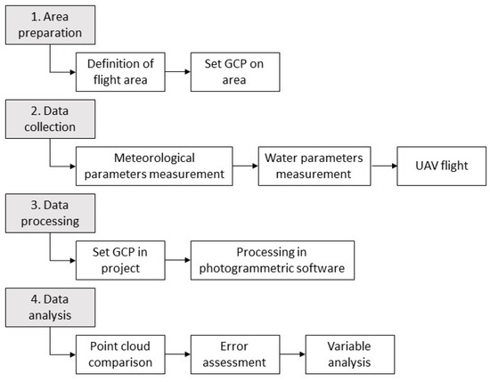
Figure 1.
Methodology flow chart.
2.2.1. Area Preparation
A survey was conducted using conventional topographic equipment in which three ground control points (GCPs) were placed outside and two control points were placed inside the underwater area (Figure 2). and georeferencing of the area was assessed through a GNSS, as is shown in Table 3 [61].
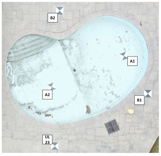
Figure 2.
Ground control points (GCPs) in the study area. A1, A2, B1, B2 and UL23 are the names of the control points.
Table 3.
Control points coordinates.
Figure 3 denotes the pool measurements and the finished floor levels (FFLs) for each pool step used as a reference in the error calculations.
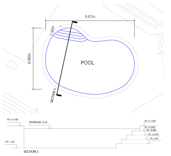
Figure 3.
Plan and section using measurements from the topographic equipment.
2.2.2. Data Collection
For this investigation, a 67.5 m2 swimming pool within the campus grounds of the University of Lima, located in Santiago de Surco, Lima, Peru, was set as the study area, as is shown in Figure 2. As Figure 4 shows, three types of flights were carried out: with an empty pool (flights 1 to 10), with the pool filled with clean water (flights 11 to 18), and with copper sulfate added to the pool water to simulate changes in the turbidity of the water (flights 19 to 26).
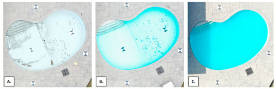
Figure 4.
(A) Empty pool. (B) Pool filled with clean water. (C) Pool filled with copper sulfate.
Copper sulfate was used to suspend particles on the water surface by dissolving the component and mixing it using a water pump. Copper sulfate (CuSO4) is an inorganic component that controls algal and plant growth in pools, lakes, and ponds [65]. However, its use in large quantities can affect the immediate turbidity of the water until it dissolves completely. It is important to note that because of the water movement and the time that elapsed during the day, different turbidity layers were present in the pool during each flight, and different tests for turbidity were performed along the pool. Water samples were taken at different pool areas for each flight to verify the turbidity levels.
When recording the climatological parameters during the flights, luminosity, wind speed, and air temperature were considered [49]. These parameters were measured for every flight. The survey flight plans were developed using the Pix4Dcapture free mobile app [64] and performed over the pool area indicated in Figure 2. Before starting these UAV flights, test flights were performed at heights of 10 m and 30 m. However, the resulting images were blurry at 10 m due to the surface proximity. In addition, the low height made recognizing the common points in the processed images difficult. Therefore, we used the following constant parameters in our flights: flight heights of 30 m and 50 m, as shown in Figure 5, 80–75% overlap, and a camera angle of 90°. Table 4 lists the 26 flights conducted based on these parameters.
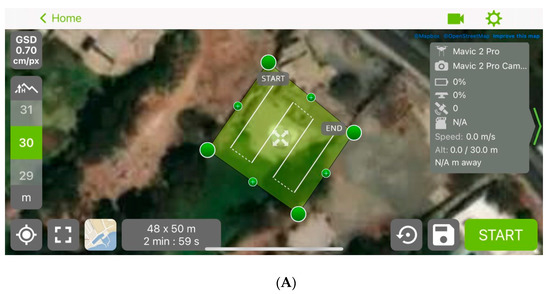
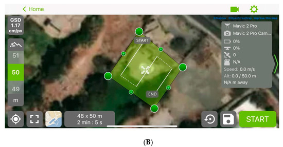
Figure 5.
(A) Flight plan at 30 m. (B) Flight plan at 50 m.
Table 4.
Selected flight parameters.
For the flights in Figure 4C, the turbidity level of the pool was managed throughout the day in NTU (nephelometric turbidity units). In Figure 6, the steps in the varying and measuring of the turbidity are denoted. During the day, pool water samples were taken before adding the copper sulfate compound to change the turbidity level of the water. The original turbidity level was set at 3.74 NTU (the World Health Organization (WHO) has established that water turbidity should not exceed 5 NTU for human consumption; however, less than 1 NTU is ideal (WHO, 2020)) for flights 11 through 18.
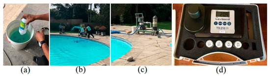
Figure 6.
Steps for changing and measuring turbidity: (a) add a copper sulfate compound to some pool water in a container; (b) pour the mixture into the pool using an electric pump; (c) recirculate the pool water with the help of an electric pump; (d) measure the water turbidity using a turbidity meter.
For flights 19 to 22, 1.5 kg of copper sulfate and pool water were mixed in a container (Figure 6a). After the component was dissolved, it was poured into the pool (Figure 6b), and an electric pump was used to recirculate the water and obtain a uniform mixture, as is shown in Figure 6c. The first turbidity test yielded an average of 20.54 NTU when recirculating the component in the pool water (Figure 6d). We then ran turbidity tests every 2 h to check whether external factors, such as light and temperature, affected the results [15,43]. Finally, for flights 23 to 26, another 1.5 kg of copper sulfate was added (making a total of 3 kg) during these tests. The average turbidity level, in this case, was 47.41 NTU.
Additionally, when recording the meteorological parameters during the flights, the parameters of luminosity, wind speed, and air temperature were considered, as is shown in Table 5 [66]. These parameters were measured at different times of the day, preferably morning, noon, and afternoon, to observe changes in the weather. The highest luminosity, between 86,700 lx and 83,400 lx, was recorded during noon, while the lowest luminosity varied between 2300 lx and 2600 lx. The wind speed remained stable during the flights (around 3 m/s). The air temperature presented a variation of 4 °C during the flights (the highest temperature recorded was 19 °C, and the lowest was 15 °C).
Table 5.
Meteorological and water parameters during the flights.
The study area was defined as an environment in which different water turbidity levels could be managed and simulated. Suspended substance particles and organic or inorganic matter might affect water clarity in a natural environment. This parameter was measured at the study site for each flight conducted, together with the other meteorological factors, since these aspects can influence the image quality when using photogrammetry [30].
2.2.3. Data Processing
In total, 26 UAV flights were performed to generate photogrammetric surveys at different degrees of water turbidity, during which flight and weather parameters were recorded. However, from flight 11 onwards, water the turbidity levels started to vary before the photogrammetric flights were conducted.
The Pix4Dmapper software [67] was used for photogrammetric processing, through which a point cloud and an orthomosaic were obtained. The information from which the images were generated was entered into the software to achieve this processing. The three control points on the dry ground were used to georeference the surveys, and the 2 control points underwater were used to determine the accuracy of the results [25]. Table 6 shows the accuracy found for each flight using the two underwater control points as reference. For flights 23 to 26, the control points could not be recognized due to the turbidity levels. Figure 7 shows the point cloud of the pool obtained from a photogrammetric flight (a), a side view of the depth of the pool (b), and a general view of the image processing with the location of the photographs, the ground control points, and the context of the study site (c).
Table 6.
Accuracy for control points underwater.
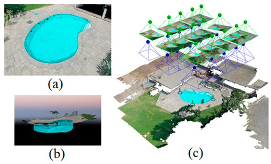
Figure 7.
Pool image processing: (a) top view of the point cloud; (b) side view of the point cloud; (c) image processing view.
Post-processing was conducted to filter the noise from the point cloud. This eliminates extreme or atypical values for the surface when obtaining photogrammetric information. Because the body being assessed is a known object on which a previous topographic survey had been conducted to determine its measurements, as is seen in Figure 7, this can be used as a foundation for noise filtering [68]. For this research, point filtering was performed manually because the case study is not a large area, and the shape of the surface is known.
3. Results
Data Analysis
Of the 26 flights realized, those flown at a height of 30 m were chosen for the study comparison. From observing the 30 m and 50 m flights, we determined that the lower resolution of the 50 m flights affected the visualization of the data and point clouds. The point clouds obtained from the thirteen 30 m flights were compared against those of the survey conducted with conventional instruments [69]. The differences found in the finished floor levels (FFL) of the steps and the bottom of the pool were used to calculate the vertical error. Figure 8 provides four examples of point clouds, wherein the red lines represent the levels obtained using a UAV and the blue lines represent the levels obtained from conventional topographic surveys. The figure shows the distortion in the point clouds for flights 11, 15, 19, and 23. The examples correspond to flights made at a height of 30 m. The point cloud from flight 11 was obtained from a pool without water and serves as a reference of the surface without distortion.
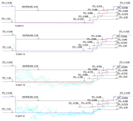
Figure 8.
Comparison between the point clouds obtained using a UAV and those obtained from conventional topographic surveys.
Since the luminosity and temperature of the remaining three flights are similar, it is easy to observe how the turbidity has changed. In these examples, the point clouds do not faithfully represent the depth of the pool. Even as the depth increases, the distortion of the point clouds increases, and the accuracy of the distances between the measured levels decreases. Flight 23 shows an extreme distortion of the point cloud, which presented levels of 47.41 NTU on average, the highest level recorded in the experiment. This result is consistent with the observations of other studies [15,29] in which the turbidity of the water directly influenced the variations in the results obtained from data collected using UVAs. This study’s high degree of innovation is worth noting, as it simulates a controlled environment. It is assumed that studies in uncontrolled environments involving water resources can be very variable and result in a high variation in errors during data collection with UVAs.
Charts were generated where the relationships between the errors obtained in the bathymetric surveys were assessed at different pool depths. The variables of depth, lux, and NTU (turbidity) were the most affected during the flight surveys. On the other hand, the wind speed and the temperature did not influence the errors since they did not vary significantly during the flights. Figure 9 presents an assessment of the errors found at different depths, considering the variation in luminosity and turbidity during the surveys. The errors found in each flight with a water-filled pool were grouped. The bars represent the luminosity level (in lux) recorded during each flight, the orange line indicates the turbidity (in NTU), and the gray line denotes the error at each depth. For example, at a constant turbidity of 4 NTU, an almost constant error is presented at each depth up to the highest luminosity, recorded at 0.73 m, which generated the highest error. Likewise, at a continuous turbidity of 21 NTU, there was a constant error up to a depth of 1.20 m, at which point the luminosity was relatively high even if it was not the highest recorded. On the other hand, when the turbidity changed from 21 NTU to 47 NTU, the error increased and the high turbidity did not allow the recording of the values for the last flight, even with a low luminosity. According to these relationships [30], it is understood that water surfaces with greater turbidity are more challenging to study with photogrammetry.
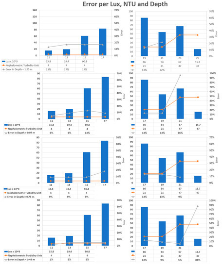
Figure 9.
Assessment of the errors found at different depths, considering the variation in luminosity and turbidity during the surveys.
Because of the refraction of light, a correction must be made due to the change in medium (air–water). Considering Snell’s law [70] and the coefficients n1 = 1 for air and n2 = 1.33 for water, it was found that the equation provides a real solution if the height difference is greater than or equal to 0.236 m. The heights obtained in this case study were smaller than those obtained in many other case studies. Because of this, and because our intention was only to study the influence of external factors on photogrammetric surveys, refraction was not considered in the comparison of the results obtained.
In a study comparing the results of photogrammetric surveys for bathymetry in coastal waters with and without GCP in the submerged area, it was found that at a depth of 0.74 m, a difference of 35.2% was obtained in the survey [71]. In this study, the error obtained at 0.73 m varied between 9% and 18% when there was a constant turbidity of 4 NTU, which was lower than the parameters recorded [71], and showed an error of 13% when presented with a level of 21 NTU. Another photogrammetry study conducted in shallow waters obtained an RSME of 0.18 m [72]. This study recorded errors between 0.023 m and 0.324 m at different depths.
Overall, the highest luminosity generated the lowest error up to a depth of 0.97 m. In addition, after assessing the variations in turbidity, two situations were observed: At shallower depths, and up to a depth of 0.49 m, the increases in turbidity positively contributed to error reduction. However, at depths exceeding 0.49 m, the increased turbidity level increased the error. This happens because in shallow waters greater turbidity decreases refraction [73]. Nevertheless, as depth increases, it becomes less relevant due to the angle, and light beams travel longer distances through the air and water [74]. These factors result in the two previously observed situations, wherein the error depends on the depth assessed, even when the same parameters are recorded in a survey [71].
Additionally, the average errors found in the underwater control points on the Z-axis of A1 and A2 were 0.04 m and 0.023 m, respectively, while X- and Y-axes presented errors under 2 cm. Unfortunately, values for the last flights couldn’t be recorded due to turbidity. This is consistent with the limitations of photogrammetry in accurately surveying coordinates on the Z-axis.
At depths exceeding 0.97 m, the effects from turbidity and luminosity cease to follow an established pattern. This is consistent with the findings of a study published by David et al. [71], which concluded that UAV photogrammetry can be applied in bathymetric surveys conducted in shallow waters that do not exceed the depth of 1 m. In addition, the authors [71] conducted flight tests in sets consisting of two or three flight repetitions under the same conditions to compensate for possible flight complications, such as poor visibility.
4. Conclusions
This study shows the limitations of photogrammetry in obtaining data on the Z-axis underwater. Control points above water and underwater provided information to compare with the values obtained from the surveys to determine the error of the photogrammetry of surfaces in shallow water. Environmental factors, such as turbidity and luminosity, affected the accuracy of the information obtained from the controlled site using the same body of water. The ground control points (GCPs) gave coordinates that allowed the point cloud to be georeferenced correctly. According to [75], three control points should be adequate to obtain an acceptable degree of precision. As Figure 2 shows, five control points were used in these experiments, and their corresponding coordinates are presented in Table 3.
On flights 23 to 26, with a turbidity of 47.41 NTU, two control points located at the bottom of the pool were no longer visible. Consequently, the values of the underwater control points could not be obtained, as is shown in Table 6.
Ref. [76] concluded that when using a UAV, there is a greater predisposition for the flight path to be influenced by the wind due to the weight of the tool and the flight height, especially when it does not have a controlled path. For this reason, the flights were carried out at heights of 30 m and 50 m over a defined section, as is shown in Table 4 and Figure 5, respectively. The wind speed remained in the range of 1 m/s to 3 m/s, with 22 of the 26 flights carried out in a wind speed of 2 m/s.
Temperature influences the operation of the UAV, especially when it is used in high temperatures. In the present study, the temperature did not affect the operation of the UAV since the flights were carried out at temperatures below 20 °C (specifically, in the range of 15 °C to 19 °C, as is shown in Table 5).
On the other hand, the results revealed that the highest luminosity generated the lowest error up to a depth of 0.97 m. In this case, two situations were observed for the turbidity variations: (1) at shallower depths (not exceeding 0.49 m), increased turbidity levels positively contributed to error reduction; and (2) at greater depths (exceeding 0.49 m), increased turbidity resulted in increased errors.
Finally, UAV-based photogrammetry can be applied, within a known margin of error, in bathymetric surveys of underwater surfaces in shallow waters not exceeding a depth of 1 m. In practice, this survey method could be applied to map shallow rivers, lakes, or coastal waters. It represents an affordable option for surveying any water rise changes or periodically monitoring soil erosion.
Further research could focus on comparing the information obtained from photogrammetry with that obtained from other bathymetric survey methods involving drones, such as those using echo sounders or integrating lidar sensors into UAV platforms [77], or even those using aerial or boat-type drones.
Author Contributions
Conceptualization, A.A.D.S. and A.L.T.; methodology, M.A.V.O. and A.L.T.; software, M.A.V.O. and G.T.U.I.; validation, A.A.D.S., A.N., A.L.T. and M.A.V.O.; formal analysis, M.A.V.O. and A.L.T.; investigation, S.R.L.R. and G.T.U.I.; resources, A.A.D.S.; data curation, A.A.D.S. and M.A.V.O.; writing—original draft preparation, S.R.L.R. and G.T.U.I.; writing—review and editing, A.A.D.S. and A.N.; visualization, S.R.L.R., G.T.U.I. and M.A.V.O.; supervision, A.A.D.S.; project administration, A.A.D.S.; funding acquisition, A.A.D.S. All authors have read and agreed to the published version of the manuscript.
Funding
This research was funded by the Scientific Research Institute (IDIC) of the Universidad de Lima under research project funding number PI.56.007.2018.
Data Availability Statement
The data supporting the findings of this study are available within the article.
Acknowledgments
The authors thank the Universidad de Lima for supporting this research.
Conflicts of Interest
The authors declare no conflict of interest.
References
- Bergsma, E.W.J.; Almar, R.; Rolland, A.; Binet, R.; Brodie, K.L.; Bak, A.S. Coastal morphology from space: A showcase of monitoring the topography-bathymetry continuum. Remote Sens. Environ. 2021, 261, 112469. [Google Scholar] [CrossRef]
- Kearns, T.A.; Breman, J. Bathymetry—The Art and Science of Seafloor Modelling for Modern Applications. Ocean Globe 2010, 1–36. [Google Scholar]
- Kapustina, M.V.; Dorokhov, D.V.; Sivkov, V.V. Multibeam bathymetry data of the western part of the Romanche Trench (Equatorial Atlantic). Data Brief 2021, 37, 107198. [Google Scholar] [CrossRef] [PubMed]
- Li, Y.; Gao, H.; Zhao, G.; Tseng, K.H. A high-resolution bathymetry dataset for global reservoirs using multi-source satellite imagery and altimetry. Remote Sens. Environ. 2020, 244, 111831. [Google Scholar] [CrossRef]
- Ang, W.J.; Park, E.; Alcantara, E. Mapping floodplain bathymetry in the middle-lower Amazon River using inundation frequency and field control. Geomorphology 2021, 392, 107937. [Google Scholar] [CrossRef]
- Ballestero, M.; García, D. Estudio Batimétrico Con Ecosonda Multihaz y Clasificación de Fondos [A Bathymetric Study Using Multi Beam Echo Sounder and Background Classification]. Bachelor´s Thesis, Universidad Politécnica de Cataluña, Barcelonam, Spain, 2010. [Google Scholar]
- Bu, X.; Yang, F.; Xin, M.; Zhang, K.; Ma, Y. Improved calibration method for refraction errors in multibeam bathymetries with a wider range of water depths. Appl. Ocean Res. 2021, 114, 102778. [Google Scholar] [CrossRef]
- Fontán, A.; Albarracín, S.; Alcántara-Carrió, J. Estudios de erosión en costas sedimentarias mediante GPS diferencial y ecosonda monohaz/multihaz [Erosion Studies on Sedimentary Coasts Using Differential GPS and Single/Multi Beam Echo Sounders]. In Métodos en Teledetección Aplicada a la Prevención de Riesgos Naturales en el Litoral [Remote Sensing Methods Applied to the Prevention of Natural Risks on the Coast]; Programa Iberoamericano de Ciencia y Tecnología para el Desarrollo: Madrid, Spain, 2009; pp. 100–122. [Google Scholar]
- Dudkov, I.Y.; Sivkov, V.V.; Dorokhov, D.V.; Bashirova, L.D. Multibeam bathymetry data from the Kane Gap and south-eastern part of the Canary Basin (Eastern tropical Atlantic). Data Brief 2020, 32, 106055. [Google Scholar] [CrossRef]
- Sun, M.; Yu, L.; Zhang, P.; Sun, Q.; Jiao, X.; Sun, D.; Lun, F. Coastal water bathymetry for critical zone management using regression tree models from Gaofen-6 imagery. Ocean Coast. Manag. 2021, 204, 105522. [Google Scholar] [CrossRef]
- Westley, K. Satellite-derived bathymetry for maritime archaeology: Testing its effectiveness at two ancient harbours in the Eastern Mediterranean. J. Archaeol. Sci. Rep. 2021, 38, 103030. [Google Scholar] [CrossRef]
- Caballero, I.; Stumpf, R.P. Retrieval of nearshore bathymetry from Sentinel-2A and 2B satellites in South Florida coastal waters. Estuar. Coast. Shelf Sci. 2019, 226, 106277. [Google Scholar] [CrossRef]
- Schwarz, R.; Mandlburger, G.; Pfennigbauer, M.; Pfeifer, N. Design and evaluation of a full-wave surface and bottom-detection algorithm for LiDAR bathymetry of very shallow waters. ISPRS J. Photogramm. Remote Sens. 2019, 150, 1–10. [Google Scholar] [CrossRef]
- Specht, C.; Świtalski, E.; Specht, M. Application of an Autonomous/Unmanned Survey Vessel (ASV/USV) in Bathymetric Measurements. Pol. Marit. Res. 2017, 24, 36–44. [Google Scholar] [CrossRef]
- He, J.; Lin, J.; Ma, M.; Liao, X. Mapping topo-bathymetry of transparent tufa lakes using UAV-based photogrammetry and RGB imagery. Geomorphology 2021, 389, 107832. [Google Scholar] [CrossRef]
- Pan, Y.; Flindt, M.; Schneider-Kamp, P.; Holmer, M. Beach wrack mapping using unmanned aerial vehicles for coastal environmental management. Ocean Coast. Manag. 2021, 213, 105843. [Google Scholar] [CrossRef]
- Del Savio, A.A.; Luna-Torres, A.; Reyes-Ñique, J.L. Implementación del Uso de Drones en Mapeo Topográfico. [Implementing the Use of Drones in Topographic Mapping] Scientific Research Institute, Universidad de Lima. 2018. Available online: https://hdl.handle.net/20.500.12724/8111 (accessed on 20 December 2022).
- Alladi, T.; Bansal, G.; Chamola, V.; Guizani, M. SecAuthUAV: A novel authentication scheme for UAV-ground station and UAV-UAV communication. IEEE Trans. Veh. Technol. 2022, 69, 15068–15077. [Google Scholar] [CrossRef]
- Krichen, M.; Adoni, W.Y.H.; Mihoub, A.; Alzahrani, M.Y.; Nahhal, T. Security Challenges for Drone Communications: Possible Threats, Attacks and Countermeasures. In 2022 2nd International Conference of Smart Systems and Emerging Technologies (SMARTTECH); IEEE: Manhattan, NY, USA, 2022; pp. 184–189. [Google Scholar]
- Manzoor, S.; Liaghat, S.; Gustafson, A.; Johansson, D.; Schunnesson, H. Establishing relationships between structural data from close-range terrestrial digital photogrammetry and measurement while drilling data. Eng. Geol. 2020, 267, 105480. [Google Scholar] [CrossRef]
- Lavaquiol, B.; Sanz, R.; Llorens, J.; Arnó, J.; Escolà, A. A photogrammetry-based methodology to obtain accurate digital ground-truth of leafless fruit trees. Comput. Electron. Agric. 2021, 191, 106553. [Google Scholar] [CrossRef]
- Kardasz, P.; Doskocz, J.; Heejduk, M.; Wiejkut, P.; Zarzycki, H. Drones and Possibilities of Their Using. J. Civ. Environ. Eng. 2016, 6, 1–7. [Google Scholar] [CrossRef]
- Addo, K.A.; Jayson-Quashigah, P.N. UAV photogrammetry and 3D reconstruction: Application in coastal monitoring. Unmanned Aer. Syst. 2021, 157–174. [Google Scholar] [CrossRef]
- Dering, G.M.; Micklethwaite, S.; Thiele, S.T.; Vollgger, S.A.; Cruden, A.R. Review of drones, photogrammetry and emerging sensor technology for the study of dykes: Best practises and future potential. J. Volcanol. Geotherm. Res. 2019, 373, 148–166. [Google Scholar] [CrossRef]
- Elkhrachy, I. Accuracy Assessment of Low-Cost Unmanned Aerial Vehicle (UAV) Photogrammetry. Alex. Eng. J. 2021, 60, 5579–5590. [Google Scholar] [CrossRef]
- Jawak, S.D.; Vadlamani, S.S.; Luis, A.J. A Synoptic Review on Deriving Bathymetry Information Using Remote Sensing Technologies: Models, Methods and Comparisons. Adv. Remote Sens. 2015, 4, 147–162. [Google Scholar] [CrossRef]
- Watanabe, Y.; Kawahara, Y. UAV Photogrammetry for Monitoring Changes in River Topography and Vegetation. Procedia Eng. 2016, 154, 317–325. [Google Scholar] [CrossRef]
- Bandini, F.; Lopez-Tamayo, A.; Merediz-Alonso, G.; Olesen, D.H.; Jakobsen, J.; Wang, S.; Garcia, M.; Bauer-Gottwein, P. Unmanned aerial vehicle observations of water surface elevation and bathymetry in the cenotes and lagoons of the Yucatan Peninsula, Mexico. Hidrogeol. J. 2018, 26, 2213–2228. [Google Scholar] [CrossRef]
- Trujillo, A.; Thurman, H. Essentials of Oceanography, 10th ed.; Pearsons Education: Upper Saddle River, NJ, USA, 2010. [Google Scholar]
- Kieu, H.T.; Law, A.W.K. Remote sensing of coastal hydro-environment with portable unmanned aerial vehicles (pUAVs) a state-of-the-art review. J. Hydro-Environ. Res. 2021, 37, 32–45. [Google Scholar] [CrossRef]
- Erena, M.; Atenza, J.F.; García-Galiano, S.; Domínguez, J.A.; Bernabé, J.M. Use of drones for the topo-bathymetric monitoring of the reservoirs of the Segura River Basin. Water 2019, 11, 445. [Google Scholar] [CrossRef]
- Mosher, D.C.; Yanez-Carrizo, G. The elusive continental rise: Insights from residual bathymetry analysis of the Northwest Atlantic Margin. Earth-Sci. Rev. 2021, 217, 103608. [Google Scholar] [CrossRef]
- Pajares, G. Overview and Current Status of Remote Sensing Applications Based on Unmanned Aerial Vehicles (UAVs). Photogramm. Eng. Remote Sens. 2015, 81, 281–330. [Google Scholar] [CrossRef]
- Laborie, J.; Christiansen, F.; Beedholm, K.; Madsen, P.T.; Heerah, K. Behavioural impact assessment of unmanned aerial vehicles on Weddell seals (Leptonychotes weddellii). J. Exp. Mar. Biol. Ecol. 2021, 536, 151509. [Google Scholar] [CrossRef]
- Hodúl, M.; Bird, S.; Knudby, A.; Chénier, R. Satellite derived photogrammetric bathymetry. ISPRS J. Photogramm. Remote Sens. 2018, 142, 268–277. [Google Scholar] [CrossRef]
- Surisetty, V.V.A.K.; Venkateswarlu, C.; Gireesh, B.; Prasad, K.V.s.R.; Sharma, R. On improved nearshore bathymetry estimates from satellites using ensemble and machine learning approaches. Adv. Space Res. 2021, 68, 3342–3364. [Google Scholar] [CrossRef]
- Dietrich, J.T. Bathymetric Structure-from-Motion: Extracting shallow stream bathymetry from multi-view stereo photogrammetry. Earth Surf. Process. Landf. 2016, 42, 355–364. [Google Scholar] [CrossRef]
- Hodúl, M.; Chénier, R.; Faucher, M.A.; Ahola, R.; Knudby, A.; Bird, S. Photogrammetric Bathymetry for the Canadian Arctic. Marine Geodesy. 2019, 43, 23–43. [Google Scholar] [CrossRef]
- Cao, B.; Fang, Y.; Jiang, Z.; Gao, L.; Hu, H. Shallow water bathymetry from WorldView-2 stereo imagery using two-media photogrammetry. Eur. J. Remote Sens. 2019, 52, 506–521. [Google Scholar] [CrossRef]
- Chénier, R.; Faucher, M.A.; Ahola, R.; Shelat, Y.; Sagram, M. Bathymetric photogrammetry to update CHS charts: Comparing conventional 3D manual and automatic approaches. ISPRS Int. J. Geo-Inf. 2018, 7, 395. [Google Scholar] [CrossRef]
- Śledź, S.; Ewertowski, M.W.; Piekarczyk, J. Applications of unmanned aerial vehicle (UAV) surveys and Structure from Motion photogrammetry in glacial and periglacial geomorphology. Geomorphology 2021, 378, 107620. [Google Scholar] [CrossRef]
- Morris, C.; Weckler, P.; Arnall, B.; Alderman, P.; Kidd, J.; Sutherland, A. Weather Impacts on UAV Flight Availability for Agricultural Purposes in Oklahoma. In Proceedings of the 13th International Conference on Precision Agriculture, St. Louis, MO, USA, 31 July–3 August 2016. [Google Scholar]
- Alam, M.S.; Oluoch, J. A survey of safe landing zone detection techniques for autonomous unmanned aerial vehicles (UAVs). Expert Syst. Appl. 2021, 179, 115091. [Google Scholar] [CrossRef]
- Ismail, A.H.; AzmI, M.S.M.; Hashim, M.A.; Ayob, M.N.; Hashim, M.S.M.; Hassrizal, H.B. Development of a webcam based lux meter. In Proceedings of the IEEE Symposium on Computers and Informatics, ISCI 2013, Langkawi, Malaysia, 7–9 April 2013; pp. 70–74. [Google Scholar] [CrossRef]
- Garilli, E.; Bruno, N.; Autelitano, F.; Roncella, R.; Giuliani, F. Automatic detection of stone pavement’s pattern based on UAV photogrammetry. Autom. Constr. 2021, 122, 103477. [Google Scholar] [CrossRef]
- Skarlatos, D.; Agrafiotis, P. A Novel Iterative Water Refraction Correction Algorithm for Use in Structure from Motion Photogrammetric Pipeline. Mar. Sci. Eng. J. 2018, 6, 77. [Google Scholar] [CrossRef]
- Zhang, D.; Fang, T.; Ai, J.; Wang, Y.; Zhou, L.; Guo, J.; Mei, W.; Zhao, Y. UAV/RTS system based on MMCPF theory for fast and precise determination of position and orientation. Measurement 2022, 187, 110342. [Google Scholar] [CrossRef]
- Mason, D.; Davenport, I.; Robinson, G.; Flather, R.; Mccartney, B. Construction of an inter-tidal digital elevation model by the ‘water-line’ method. Geophys. Res. Lett. 1995, 22, 3187–3190. [Google Scholar] [CrossRef]
- Bandini, F.; Sunding, T.P.; Linde, J.; Smith, O.; Jensen, I.K.; Köppl, C.J.; Butts, M.; Bauer-Gottwein, P. Unmanned Aerial System (UAS) observations of water surface elevation in a small stream: Comparison of radar altimetry, lidar and photogrammetry techniques. Remote Sens. Environ. 2020, 237, 111487. [Google Scholar] [CrossRef]
- Furlan, L.M.; Moreira, C.A.; Alencar, P.G.; Rosolen, V. Environmental monitoring and hydrological simulations of a natural wetland based on high-resolution unmanned aerial vehicle data (Paulista Peripheral Depression, Brazil). Environ. Chall. 2021, 4, 100146. [Google Scholar] [CrossRef]
- Villarreal, C.A.; Garzón, C.G.; Mora, J.P.; Rojas, J.D.; Ríos, C.A. Workflow for capturing information and characterizing difficult-to-access geological outcrops using unmanned aerial vehicle-based digital photogrammetric data. J. Ind. Inf. Integr. 2021, 26, 100292. [Google Scholar] [CrossRef]
- Zhang, D.; Watson, R.; Dobie, G.; Macleod, C.; Khan, A.; Pierce, G. Quantifying impacts on remote photogrammetric inspection using unmanned aerial vehicles. Eng. Struct. 2020, 209, 109940. [Google Scholar] [CrossRef]
- Tao, X.; Li, Y.; Yan, W.; Wang, M.; Tan, Z.; Jiang, J.; Luan, Q. Heritable variation in tree growth and needle vegetation indices of slash pine (Pinus elliottii) using unmanned aerial vehicles (UAVs). Ind. Crops Prod. 2021, 173, 114073. [Google Scholar] [CrossRef]
- Kreij, A.; Scriffignano, J.; Rosendahl, D.; Nagel, T.; Ulm, S. Aboriginal stone-walled intertidal fishtrap morphology, function and chronology investigated with high-resolution close-range Unmanned Aerial Vehicle photogrammetry. J. Archaeol. Sci. 2018, 96, 148–161. [Google Scholar] [CrossRef]
- Ali-Sisto, D.; Gopalakrishnan, R.; Kukkonen, M.; Savolainen, P.; Packalen, P. A method for vertical adjustment of digital aerial photogrammetry data by using a high-quality digital terrain model. Int. J. Appl. Earth Obs. Geoinf. 2020, 84, 101954. [Google Scholar] [CrossRef]
- DJI Mavic 2 Specs. Available online: https://www.dji.com/mavic-2/info (accessed on 9 March 2020).
- Vellemu, E.C.; Katonda, V.; Yapuwa, H.; Msuku, G.; Nkhoma, S.; Makwakwa, C.; Safuya, K.; Maluwa, A. Using the Mavic 2 Pro drone for basic water quality assessment. Sci. Afr. 2021, 14, 00979. [Google Scholar] [CrossRef]
- Outay, F.; Mengash, H.A.; Adnan, M. Applications of unmanned aerial vehicle (UAV) in road safety, traffic and highway infrastructure management: Recent advances and challenges. Transp. Res. Part A Policy Pract. 2020, 141, 116–129. [Google Scholar] [CrossRef]
- Turbidímetro para Aguas TB 210 IR. Available online: https://giardinoperu.com/producto/tb-210-ir-lovibond (accessed on 9 March 2020).
- Amprobe LM-200LED LED Light Meter. Available online: http://content.amprobe.com/DataSheets/LM-200LED%20Light%20Meter.pdf (accessed on 9 March 2020).
- TOPCON Hiper VR GNSS Receiver. Available online: https://www.topconpositioning.com/es/support/products/hiper-vr (accessed on 20 October 2019).
- Ajayi, O.G.; Palmer, M.; Salubi, A.A. Modelling farmland topography for suitable site selection of dam construction using unmanned aerial vehicle (UAV) photogrammetry. Remote Sens. Appl. Soc. Environ. 2018, 11, 220–230. [Google Scholar] [CrossRef]
- Zolkepli, M.F.; Ishak, M.F.; Yunus, M.Y.M.; Zaini, M.S.I.; Wahap, M.S.; Yasin, A.M.; Sidik, M.H.; Hezmi, M.A. Application of unmanned aerial vehicle (UAV) for slope mapping at Pahang Matriculation College, Malaysia. Phys. Chem. Earth Parts A/B/C 2021, 123, 103003. [Google Scholar] [CrossRef]
- Pix4Dcapture. Available online: https://www.pix4d.com/es/producto/pix4dcapture (accessed on 19 August 2020).
- Song, L.; Marsh, T.L.; Voice, T.C.; Long, D.T. Loss of seasonal variability in a lake resulting from copper sulfate algaecide treatment. Phys. Chem. Earth Parts A/B/C 2011, 36, 430–435. [Google Scholar] [CrossRef]
- Meneses, N.C.; Baier, S.; Reidelstürz, P.; Geist, J.; Schneider, T. Modelling heights of sparse aquatic reed (Phragmites australis) using Structure from Motion point clouds derived from Rotary- and Fixed-Wing Unmanned Aerial Vehicle (UAV) data. Limnologica 2018, 72, 10–21. [Google Scholar] [CrossRef]
- Pix4Dmapper. Available online: https://www.pix4d.com/es/producto/pix4dmapper-fotogrametria-software (accessed on 19 August 2020).
- Mateus, S.; Sánchez, G.; Willian Branch, J.; Boulanger, P. Selección de puntos representativos en imágenes de rango. [Selection of Representative Points in Range Images]. Rev. Ing. Univ. De Medellín 2006, 5, 147–158. Available online: https://www.redalyc.org/articulo.oa?id=75050812 (accessed on 20 December 2022).
- Jeong, G.Y.; Nguyen, T.N.; Tran, D.K.; Hoang, T.B.H. Applying unmanned aerial vehicle photogrammetry for measuring dimension of structural elements in traditional timber building. Measurement 2020, 153, 107386. [Google Scholar] [CrossRef]
- Winkler, J. Snell’s Law 1 Optics. 2017. Available online: https://www.researchgate.net/publication/337486003_Snell%27s_Law_1_Optics?channel=doi&linkId=5ddb8f46a6fdccdb4462c979&showFulltext=true (accessed on 15 August 2021). [CrossRef]
- David, C.G.; Kohl, N.; Casella, E.; Rovere, A.; Ballesteros, P.; Schlurmann, T. Structure-from-Motion on shallow reefs and beaches: Potential and limitations of consumer-grade drones to reconstruct topography and bathymetry. Coral Reefs 2021, 40, 835–851. [Google Scholar] [CrossRef]
- Genchi, S.A.; Vitale, A.J.; Perillo, G.M.; Seitz, C.; Delrieux, C.A. Mapping Topobathymetry in a Shallow Tidal Environment Using Low-Cost Technology. Remote Sens. 2020, 12, 1394. [Google Scholar] [CrossRef]
- Murase, T.; Tanaka, M.; Tani, T.; Miyashita, Y.; Ohkawa, N.; Ishiguro, S.; Suzuki, Y.; Kayanne, H.; Yamano, H. A photogrammetric correction procedure for light refraction effects at a two-medium boundary. Photogramm. Eng. Remote Sens. 2008, 74, 1129–1136. [Google Scholar] [CrossRef]
- Agrafiotis, P.; Skarlatos, D.; Georgopoulos, A.; Karantzalos, K. Shallow water bathymetry mapping from UAV imagery based on machine learning. Int. Arch. Photogramm. Remote Sens. Spat. Inf. Sci. 2019, 2, 9–16. [Google Scholar] [CrossRef]
- Tellidis, I.; Levin, E. Photogrammetric image acquisition with small unmanned aerial systems. In Proceedings of the ASPRS 2014 Annual Conference, Louisville, KY, USA, 23–28 March 2014. [Google Scholar]
- Wang, B.H.; Wang, D.B.; Ali, Z.A.; Ting Ting, B.; Wang, H. An overview of various kinds of wind effects on unmanned aerial vehicle. Meas. Control 2019, 52, 731–739. [Google Scholar] [CrossRef]
- Del Savio, A.A.; Luna Torres, A.; Chicchón Apaza, M.A.; Vergara Olivera, M.A.; Llimpe Rojas, S.R.; Urday Ibarra, G.T.; Reyes Ñique, J.L.; Macedo Arevalo, R.I. Integrating a LiDAR Sensor in a UAV Platform to Obtain a Georeferenced Point Cloud. Appl. Sci. 2022, 12, 12838. [Google Scholar] [CrossRef]


Disclaimer/Publisher’s Note: The statements, opinions and data contained in all publications are solely those of the individual author(s) and contributor(s) and not of MDPI and/or the editor(s). MDPI and/or the editor(s) disclaim responsibility for any injury to people or property resulting from any ideas, methods, instructions or products referred to in the content. |
© 2023 by the authors. Licensee MDPI, Basel, Switzerland. This article is an open access article distributed under the terms and conditions of the Creative Commons Attribution (CC BY) license (https://creativecommons.org/licenses/by/4.0/).