Uncertainty Analysis of Spherical Joint Three-Dimensional Rotation Angle Measurement

Abstract

A precision spherical joint is a type of spherical motion pair that can realize three degrees of rotation freedom. In this paper, a specific method is used to assess the uncertainty of our measurement system. The measurement system uses the codes and eddy current sensor to measure the angle. Different codes are engraved on the surface of the spherical joint. Eddy current sensors are embedded in the spherical socket to detect and recognize the spherical code. The uncertainty of the measurement system hardware and an artificial neural network are studied. Based on the Monte Carlo method, the uncertainty components are evaluated and combined, and the comprehensive uncertainty of the measurement system is obtained. The evaluation results of system measurement uncertainty are verified from specific angles. In the three-axis measurement uncertainty, the minimum is about 2′, and the maximum uncertainty is about 1°. The proposed method can be used to evaluate the uncertainty of other multiple-input multiple-output measurement systems.

1. Introduction

In modern measurement systems, the multi-input multi-output measurement model is widely used. In practical work and learning, many factors usually affect the output of dependent variables, and many independent variables often interact with each other in the measurement system. A series of measurement systems, such as the geometrical deviation modeling of a 3D surface [1], fault detection, diagnosis in large-scale multi-machine power systems [2], wireless power combining and delivering systems [3], polarization angle estimation of radar [4], and the evaluation of alpha-synuclein aggregation states [5] are examples of multi-input multi-output measurement models. The quality of the measurement system can be understood by the uncertainty evaluation of the system.

The uncertainty evaluation methods of multiple-input and multiple-output measurement systems usually include the Monte Carlo method (MCM), Bayesian probability, and indirect evaluation methods based on neural networks. Kai Wang et al. [6] used an uncertainty evaluation method of an adaptive neural network algorithm to obtain the uncertainty value of the fringe image center extraction measurement system in real time. Ke Zhang et al. [7] studied the evaluation of the roundness error by comparing the Bayesian method with the method provided by ISO. Bin Zhang et al. [8] proposed a probabilistic neural network with Gaussian mixture distribution parameters to improve the detection accuracy of manufactured porosity monitoring systems and obtain confidence intervals. Luyao Liu et al. [9] established the weight change combined prediction model by using the genetic algorithm optimized back propagation method. Yuchi Ma et al. [10] established a Bayesian network to predict the corn yield in the United States and evaluate the uncertainty of the prediction.

Shenlong Wang et al. [11] used the backpropagation neural network and least squares support vector machine to establish a mathematical model, verified the accuracy of the model, and proved the effectiveness of MCM in the whiplash test model. Davor Antanasijevic et al. [12] evaluated the uncertainty of various influencing factors by using the Monte Carlo method through the uncertainty analysis of dissolved oxygen in Danube River water in Serbia. Mou Jiapeng et al. [13] proposed an uncertainty evaluation method of a fiber optic gyroscope angle measuring system based on MCM for angle transmission and traceability technology. Zhen ying Cheng et al. [14] used MCM to evaluate and combine the uncertainty of obtained model parameters and verified its effectiveness in evaluating the uncertainty of a sensor dynamic system. Dennis Madsen [15] demonstrates how the posterior distribution can be used to build shape models that better generalize and visualize the uncertainty in the established correspondence. Ke Zhang [16] presents a dynamic evaluation model of Markov chain Monte Carlo (MCMC) roundness error measurement uncertainty based on a stochastic process. Hyung-Seok Shim [17] uses the MCMC method to calculate the uncertainty of the measurement reliability model and the optimal calibration interval. Yaru Li [18] uses the Monte Carlo method (MCM) and AMCM to evaluate the uncertainty of pose results.

The above methods of uncertainty evaluation, based on neural networks and the Bayesian method, were too complicated, the technical threshold was high, and the sources of uncertainty were not considered comprehensively. For a dynamic measurement system with multiple inputs and multiple outputs, the uncertainty factors of measurement results were complex, and quantifying the influence of various error sources on measurement results, as well as and carrying out error transmission, is difficult. Therefore, MCM is more suitable to evaluate the quality of the measurement results of such systems.

In the early stage, our team developed 2D or 3D rotation angle measurement systems based on the magnetic effect method and the combination of eddy current sensors and pseudorandom coding [19,20,21]. The magnetic effect method measures the value of the magnetic field. A magnet was placed at the bottom of the spherical join. The magnetic field change was measured using a gauss meter as the spherical joint turned. The artificial neural network is used to establish the measurement model of the measured magnetic field value and the rotation angle. To further improve the accuracy of the angle measurement system, this study investigated its α, β, and γ three-axis uncertainty. The minimum accuracy of the three-axis uncertainty is about 2′, and the maximum is about 1°.

The remainder of this paper is structured as follows. The Section 2 introduces the principle of the measurement scheme and the experimental results, the Section 3 analyzes the sources of errors affecting the evaluation of uncertainty, the Section 4 shows the process of estimation uncertainty, and the Section 5 draws the conclusions.

2. Principle and Experiment

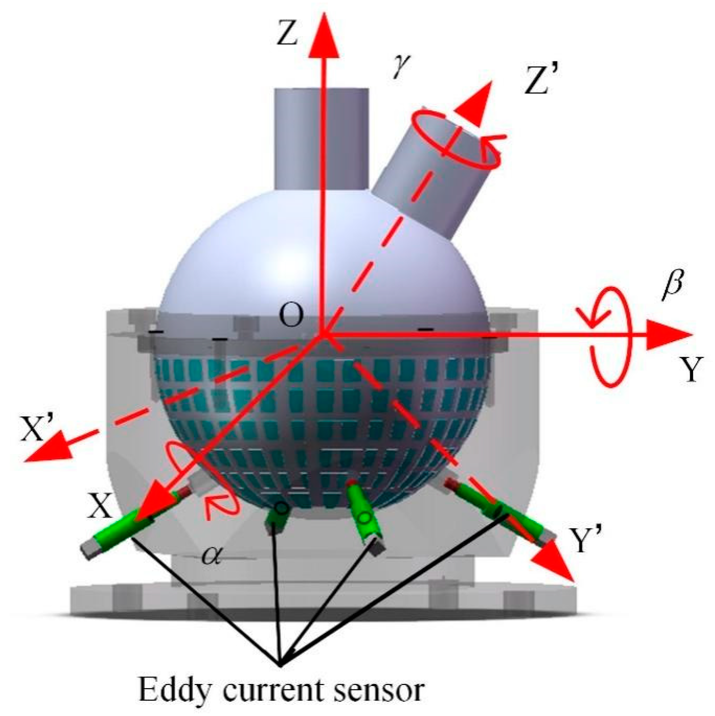
2.1. Principle

The team proposed a 3D angle detection theory and method based on spherical stereo coding and an eddy current sensor array [22]. In order to ensure that the rotation angle has a one-to-one mapping relationship with the output of the eddy current, a pseudo-random code method is mapped onto the sphere using the planar pseudo-random code. The pseudo-random sequence is a periodic sequence composed of 0 and 1, which is a kind of predetermined structure. The sequence can be copied or repeated, and exhibits the random character of the encoding.

Based on the theory of pseudorandom coding, we designed a pseudorandom 3D spherical coding and then identify spherical coding through a sensor array to detect the comprehensive changes caused by the morphologies of spherical head rotation. The key thinking behind measuring the rotary angle of a spherical joint using an eddy current sensor is to use the sensor probe to sweep the comprehensive change in the sensor output signal when different position codes, contours, and groove depths are scanned. As the eddy current meets the groove, according to the eddy current effect, when the spherical joint rotates, the sensor output will change, so as to reflect the surface characteristics of the spherical joint surface changes. By identifying and reading the code of the spherical joint, the network measurement model of the rotary angle and eddy current output of the spherical joint are established. We obtained the output value of the eddy current sensor array through external acquisition as the input and used the rotation angle value provided by a three-dimensional rotary table as the output. The artificial neural network was used to train the measurement model. The position and pose of the smart spherical joint are shown in Figure 1. Based on the right-hand principle, the reference coordinate system O-XYZ is established, with the center O of the ball as the origin. When the ball head rotates within the ball and socket for three degrees of freedom, its rotation position can be broken down into α, the rotation angle at the X axis; β, the rotation angle at the Y axis; and γ, the rotation angle at the club axis.

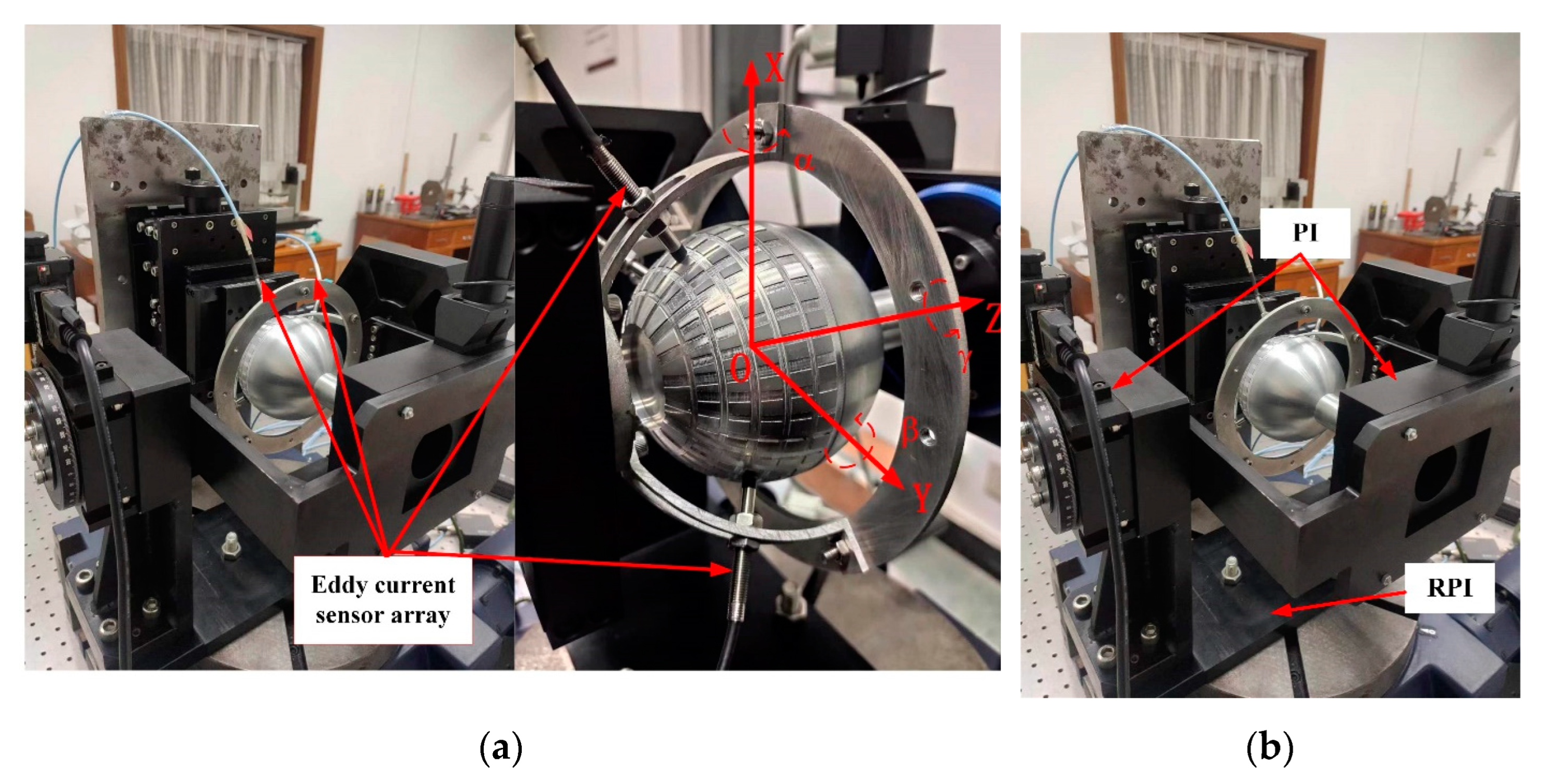
2.2. Measurement System and Data Acquisition

The experimental device is shown in Figure 2. Three single-axis precision rotary tables are used, namely, continuous, PI and RPI, to provide the step by step standard rotary angle values of three axes, with accuracies of ±4″, ±2″, and ±1″, respectively. Four eddy current sensors are employed and asymmetrically located by the fixture. The sensor probe is fixed by the nut through the arc plate, and the sensor array probe points to the ball center of the spherical joint. The position of the sensor is shown in Figure 3. The angles between the sensors are 60°, 75°, 90°, and 135°. The arc-shaped plate has a ring groove, and its pitch angle ranges from 120° to 150°. The rotation deviations of the ball head within the rotation range of the X, and Y axes and the ball joint rod are 39 μm, 38 μm, and 23 μm.

The output value of the eddy current sensor is the voltage signal. The data is collected by an NI acquisition card and stored in an Excel table by LabVIEW software. The standard angle of three-axis rotation is provided by the three-dimensional rotary table. The neural network was used to train the measurement model, with the collected eddy current voltage as the input and the three-dimensional rotation angle as the output. During the experiment, three standard angle values provided by the three rotary tables and the output values of the eddy current sensor are mapped into data groups one by one to facilitate the subsequent artificial neural network model training.

2.3. Generalized Regression Neural Network Data Processing

Our previous study found that the general regression neural network (GRNN) showed better training performance. Therefore, the GRNN algorithm was used to process the data; then, a neural network measurement model of eddy current–rotation angle was established. The measurement model uses the value output from the eddy current sensor as the input and the standard angle provided by the three-dimensional rotary table as the output. A total of 21 × 21 × 121 groups of sensor data are collected and used to train the neural networks. The data group is divided into four regions due to the large amount of data. The dataset includes 21 × 21 × 121 = 53,361 sets of an input vector of size 4 × 1 and an output vector of size 3 × 1. According to the measurement range α and β, the overall amount of data is evenly distributed into four quadrants.

The structure of the GRNN is shown in Figure 4. In the network model, the voltage value as the input matrix of the network is ${[{\mathrm{U}}_1,{\mathrm{U}}_2,{\mathrm{U}}_3,{\mathrm{U}}_4]}^{\mathrm{T}}$, and the angle as the output matrix is ${[\mathsf{\alpha },\mathsf{\beta },\mathsf{\gamma }]}^{\mathrm{T}}$. The number of neurons in the pattern layer is the same as the number of trained datasets. Its neuron transfer function can be expressed as:

$${\mathrm{R}}_{\mathrm{i}}=\mathrm{e}\mathrm{x}\mathrm{p}[-\frac{{\Vert \mathrm{V}-{\mathrm{V}}_{\mathrm{i}}\Vert }^2}{2{\mathsf{\sigma }}_{\mathrm{i}}^2}] \mathrm{i}=1,2,\mathrm{L},\mathrm{n}$$

(1)

There are two types of neurons in the summation layer of GRNN. In the first type, the output of neurons in the pattern layer is directly summed, and the connection weight with neurons in the pattern layer is 1. The output S_D is expressed as:

$$S_D={\displaystyle \sum _{i=1}^{n}exp[-\frac{{(V-V_i)}^T(V-V_i)}{2{\mathsf{\sigma }}^2}]}$$

(2)

The second type is a weighted summation of the output of the pattern layer neuron. The neuron output has the same dimension as the sample output, and each neuron represents a certain dimension of the output. The connection weight of neurons in the pattern layer is the output value of this dimension of all samples. It can be expressed S_{N j} as:

$$S_{Nj}={\displaystyle \sum _{i=1}^n{y}_{ij}exp[-\frac{{(V-V_i)}^T(V-V_i)}{2{\mathsf{\sigma }}^2}]}\hspace{1em}j=1,2,L,k$$

(3)

In the output layer, the neuron number is equal to the output vector dimensions, and each neuron output is as follows:

$$y_j=\frac{S_{Nj}}{S_D}\hspace{1em}j=1,2,\dots ,k$$

(4)

Taking the data of the third quadrant 10° ≤ α ≤ 0 and −10 ≤ β ≤ 0 as examples, to better observe the actual measurement results of the three axes, three-dimensional rotation angle measurement results of the spherical joint are drawn, respectively, based on the GRNN neural network model. As shown in Figure 5 below, when the horizontal and vertical coordinates are the standard angle, the vertical coordinate is the actual measured value of this dimension. Figure 5a shows the specific test values of α angle when the measuring range is 0° ≤ γ ≤ 120° and −10° ≤ β ≤ 0°. The values on the axis represent the standard angular rotation values provided, and the actual values are the neural network test values. Figure 5b shows the specific test values of the β angle, and Figure 5c shows the specific test values of the γ angle. All experimental data were processed. The result of α, β, and γ of the mean square error of measurement were respectively 11′55″, 10′18″, and 37′44″.

3. Uncertainty Analysis of Spherical Joint Space Rotation Measurement System

The total measurement system is composed of a three-dimensional rotation calibration table, a spherical joint, an eddy current sensor, a data acquisition card, and computer software and hardware. Theoretically, each part of the measurement chain will introduce error sources and generate uncertainty components. From the angle of error propagation, each error source contributes to the measurement uncertainty of the measurement system, according to the propagation law of uncertainty.

3.1. Source Analysis of Uncertainty under Specific Angle Measurement

In the measurement process, the ball head is made of aluminum. At 20 °C the temperature coefficient of aluminum is 2.3 × 10⁻⁵/°C [23], and the experiment is carried out in a constant temperature laboratory, so the influence of temperature on the deformation of the ball head can be ignored. In the design scheme, the eddy current sensor is used to sweep through different contours and grooves. Neural network modeling was used to fit the spherical surface morphology and the corresponding rule of the sensor array output value. The influence of the surface machining error of the ball head has good fault tolerance, and the uncertainty caused by the surface machining error of the ball head can be ignored.

Based on the uncertainty analysis of the measurement system mentioned above, the uncertainty of the spherical joint space rotation measurement system mainly comes from the errors of the three-dimensional rotary calibration table, the ball head eccentricity, the sensor errors, and the neural network model errors. The influence of sensor errors and model errors on the sampling points can be analyzed in combination.

According to the concept of MCM simulation, the general form of the uncertainty model of the spherical joint rotation measurement system can be summarized as follows:

$$y=Y+u_1+u_2+u_3$$

(5)

where:

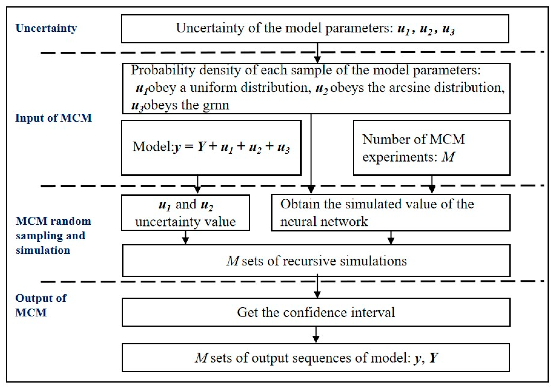
• y—measurement results synthesized according to the uncertainty model;
• Y—results obtained through measurement model calculation;
• u₁—the uncertainty component of the calibration platform rotation;
• u₂—the uncertainty component of ball head eccentricity;
• u₃—the uncertainty component of the sensor and neural network measurement model.

3.2. Uncertainty Caused by Calibration Platform Rotation Error

According to the technical specifications provided by the manufacturer of the 3D rotary calibration table, the RPI rotary table provides the standard rotation angle of the ball head around the X axis, α, and the rotation accuracy is ±1″. The induction synchronizer shows the standard rotation angle of the ball head around the Y axis, β, with accuracy up to ±3.6″. The PI rotary table provides the standard rotation angle of the ball head around the spherical joint rod itself, γ, with an accuracy of ±2″. By three-dimensional rotary calibration, error u₁ can be caused by the assumption of uniform distribution.

$$u_1(\mathsf{\alpha })~U(-1″,1″)$$

(6)

$$u_1(\mathsf{\beta })~U(-3.6″,3.6″)$$

(7)

$$u_1(\mathsf{\gamma })~U(-2″,2″)$$

(8)

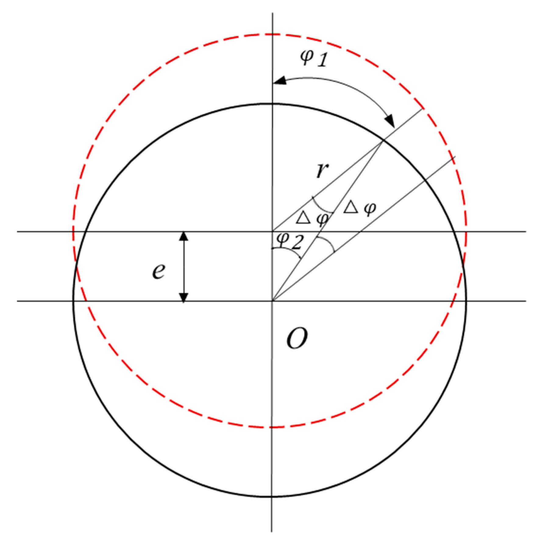
3.3. Uncertainty Caused by Ball Head Eccentricity

The eccentricity error is caused by the non-coincidence between the center of the rotation of the measuring system and the center of the ball-hinge prototype. The eccentricity error would cause the deviation of the actual distance between the probe of the eddy current sensor and the surface of the ball head, bringing additional variation to the sensor signal. In Figure 6, let ${\phi }_1$ be the rotation angle of the ball head prototype with a theoretical ball center and ${\phi }_1$ be the rotation angle of the ball head prototype with an eccentric ball center, with the radius of the ball head r = 50 mm.

The simplified eccentricity error formula is shown in Equation (5) [24].

$$\frac{sin\mathsf{\Delta }\mathsf{\phi }}{sin{\mathsf{\phi }}_2}=\frac{e}{r}$$

(9)

It can be written as:

$$\mathsf{\Delta }\mathsf{\phi }=arcsin\left(\frac{e}{r}sin{\mathsf{\phi }}_2\right)$$

(10)

Equation (6) shows that the eccentricity error changes sinusoidally when ${\phi }_2$ = 90° or 270°. The absolute value reaches its maximum:

$$\mathsf{\Delta }{\mathsf{\phi }}_{{}_{max}}=arcsin\frac{e}{r}$$

(11)

The eccentricity of the three-dimensional rotation of the joint is measured by the dial meter. The rotation deviation of the ball head within the rotation range of the X, Y axes and the ball joint rod is 39 μm, 38 μm, and 23 μm, respectively. The value also includes the roundness error of the ball head, that is, the real eccentricity error is less than the value. However, for the convenience of analysis, the maximum eccentricities around the X, Y axes and the ball joint, which are ±2′41″, ±2′37″, and ±1′35″, respectively, can be directly calculated according to Formula (7). The uncertainty u₂ follows the arcsine distribution, and the interval half-width is the absolute value of the maximum eccentricity.

$$u_2\left(\mathsf{\alpha }\right)~arcsin(-2\prime 41″,2\prime 41″)$$

(12)

$$u_2\left(\mathsf{\beta }\right)~arcsin(-2\prime 37″,2\prime 37″)$$

(13)

$$u_2\left(\mathsf{\gamma }\right)~arcsin(-1\prime 35″,1\prime 35″)$$

(14)

3.4. Uncertainty Caused by Network Model and Sensor

The output measurement data of the eddy current sensor will be processed by the neural network measurement model. Its own uncertainty will be carried into the final measurement results through calculation. The sensor repeatability error and the uncertainty introduced by the network model can be evaluated by MCM. The neural network measurement model can be expressed as:

$$\mathrm{y}\prime (\mathsf{\alpha },\mathsf{\beta },\mathsf{\gamma })=f\left(v_1,v_2,v_3,v_4,\omega \right)$$

(15)

$v_1,v_2,v_3,v_4$ are the output values of four eddy current sensors, and $\omega$ represents the network parameters in the neural network measurement model. Inputs $v_1,v_2,v_3,v_4$ $\omega$ are the main factors affecting the uncertainty of the model. $\omega$ is the smoothing factor in the neural network, which is the overall factor affecting the measurement uncertainty in the transmission process. The smoothing factor $\omega$ was used to determine the best measurement model. The “f” represents the GRNN model. The equation shows that the measured α, β, and γ can be obtained through the mathematical model. The mathematical model means the measurement model trained by GRNN. The uncertainty of the measured 3D angle is also calculated indirectly by each input through a mathematical model. The steps for evaluating the measurement system using MCM are shown in Figure 7.

The output of the sensor changes continuously with the range detected, and the error shows a random state. According to prior analysis, it can be preliminarily assumed that it is subject to an approximately normal distribution.

The normal test of the input is carried out, so the output data of the sensor in a period is sampled. For (−5°, −5°, 0°), the third quadrant midpoint, 10 data samples were taken from the 4 sensor arrays, with a single sample size of 3448. Given that the sample size is less than 5000, the Shapiro–Wilk test [25], which is suitable for small sample sizes, was used. The S–W test was performed on the output samples of four sensors, S1, S2, S3, and S4, and the results are shown in

Table 1. Sensor output distribution table.

Sensor Model	The Average	The Standard Deviation	Skewness	Kurtosis	S–W Test
S1	6.627	0.003	0.12	−0.523	0.994 (0.000 ***)
S2	3.470	0.001	0.049	0.075	0.999 (0.010 **)
S3	2.190	0.001	0.146	−0.085	0.998 (0.000 ***)
S4	6.098	0.001	−0.085	−0.207	0.997 (0.000 ***)

Note: ***, ** represent the significance level of 1%, 5% respectively.

. The data of S1, S2, S3, and S4 were the output of the sensor.

According to Table 1, for samples S1, S2, S3, and S4, the statistical values of the normality test results were 0.994, 0.999, 0.998, and 0.997, indicating strong correlations. The data do not meet the normal distribution, but their absolute kurtosis values are all less than 10, and their absolute skewness values are all less than 3. Therefore, the normal distribution histogram and the P–P diagram can be combined for further analysis. The distribution of the four sensors is similar. Therefore, taking sensor S1 as an example, the normality test histogram of S1 is shown in Figure 8.

The normal graph presents a bell shape (high in the middle and low at both ends), indicating that although the data are not absolutely normal, they can be accepted as having a normal distribution. A P–P graph is a type of chart drawn according to the relationship among the cumulative proportion of variables and the cumulative proportion of the specified distribution. As shown in Figure 9, the coincidence degree of scatter and straight lines is relatively high. The deviation from the line of normal cumulative probability was in the range of 0.02. Therefore, it can be considered to obey a normal distribution.

According to the Monte Carlo method, the probability density function is clearly known and the statistical calculation is carried out. Therefore, it is verified that the sensor and the neural network obey the normal distribution at specific points.

The sensor S₁ and the mean value and standard deviation (SD) of 9 sampled data are shown in

Table 2. Statistics table for S₁.

Sampling of S1	Data 1	Data 2	Data 3	Data 4	Data 5	Data 6	Data 7	Data 8	Data 9
Average (V)	6.6246	6.6645	6.6697	6.6269	6.6277	6.6105	6.6282	6.6629	6.6613
The SD(V)	0.0063	0.0025	0.0059	0.0026	0.0014	0.0082	0.0012	0.0012	0.0034

. The data in Table 2 was the output of sampling of S₁.

The above data indicate that the actual mean value and variance differ greatly, so the process is not an ergodic process of each state. Given that the difference between the variances of all parties is less than 0.007 V, the variances can be considered consistent. Therefore, this random process can be judged as a general stationary process, and the evaluation parameter of an error sample can be used to replace the evaluation parameter of the population average. Table 2 determines whether the sample mean data can be used to replace the overall mean data.

4. Evaluation of Measurement Uncertainty at Specific Angles

In the early data processing, the data group is divided into four regions. In the subsequent uncertainty analysis, points in four different regions were selected for evaluation.

The sample data of angles at (−5°, −5°, 0°), (−5°, 5°, 5°), (5°, −5°, 0°), and (5°, 5°, 5°) were selected, and the measurement uncertainty was evaluated by MCM, including the three-dimensional rotary calibration table, ball head eccentricity error, sensor repeatability error, and network model introduction. Taking (−5°, −5°, 0°), the third quadrant midpoint, as an example, the evaluation process was as follows.

(1)

After optimizing the parameters of the measurement model based on GRNN, the ω value was determined, which was the optimal network measurement model.

(2)

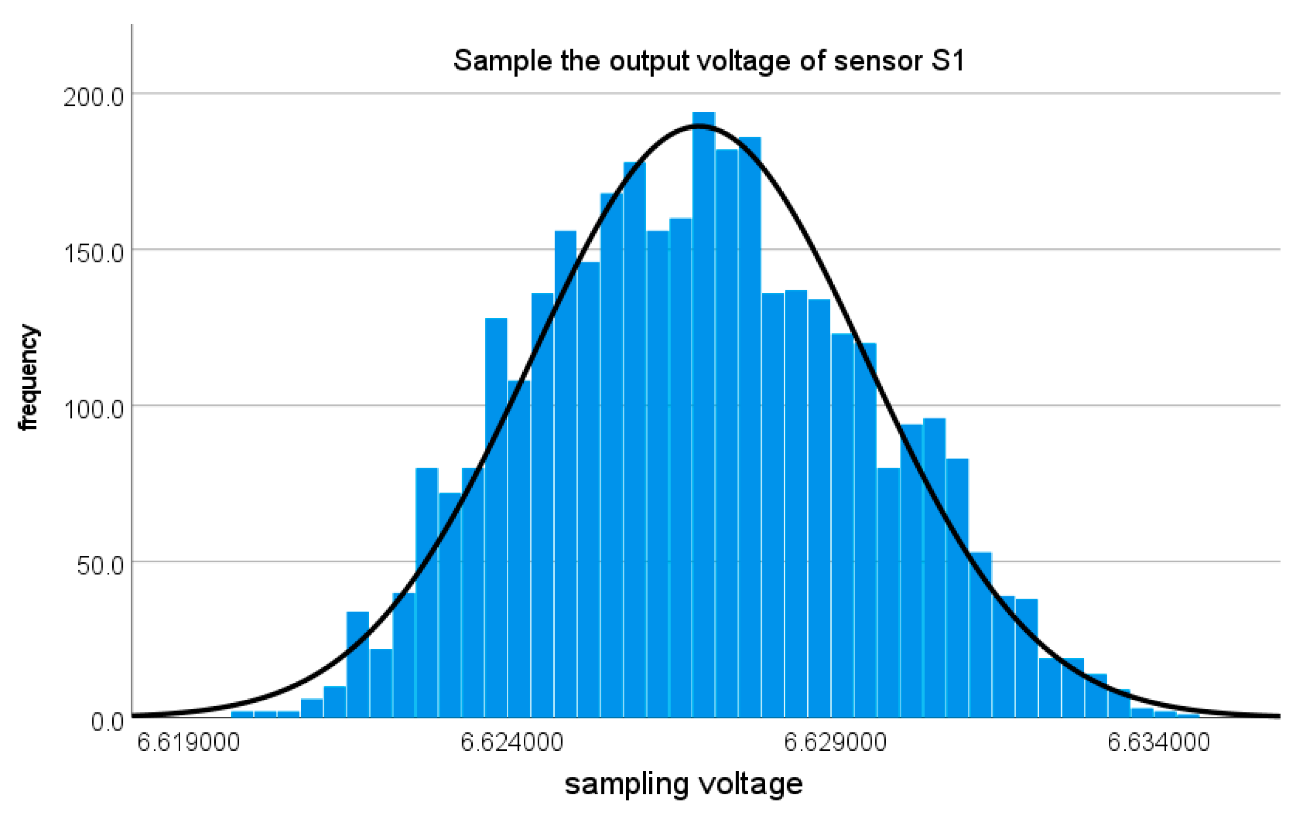
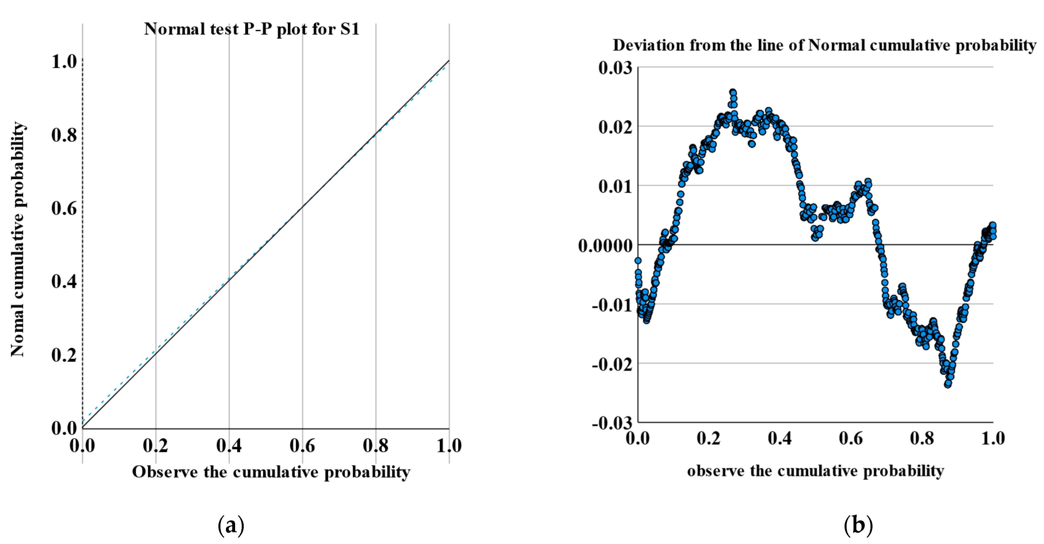
The probability density function of each input value of the sensor array is determined as S1~N (−1.9587, 0.00102), the input S2~N (−1.6779, 0.00122), the input S3~N (2.4394, 0.00102), and the input S4~N (−3.5227, 0.00112).

(3)

When setting random sampling times, M = 10⁶, S1, S2, S3, and S4 are randomly selected through random M number generation in MATLAB and put into a well-trained neural network measurement model to obtain M (α, β, and γ) sample values which contain both the sensor and the neural network’s own uncertainty.

(4)

The above two sections show that the rotation errors caused by the errors of the three-dimensional rotary calibration table are respectively $u_1(\alpha )$ subjected to U(−1″, 1″), $u_1(\beta )$ subjected to U(−3.6″, 3.6″), and $u_1(\gamma )$ subjected to U(−2″, 2″). The rotation errors caused by the ball head eccentricity error are as follows: $u_2(\alpha )$ obeys the arcsine distribution (−2′41″, 2′41″), $u_2(\beta )$ obeys the arcsine distribution (−2′37″, 2′37″), and $u_2(\gamma )$ obeys the arcsine distribution (−1′35″, 1′35″).

(5)

M random simulation samples are performed separately, assuming that the items are independent of each other, and are calculated according to Equation (5), with the sample values (α″, β″, γ″) of (α, β, and γ).

(6)

According to the algorithm steps of the Monte Carlo method, the final result of calculating the average of 106 simulation calculations yields α, β, γ at (−5°, −5°, 0°), the optimal estimate of the measured value at (−5°, −58′51″, −4°59′59″, 0°11′12″), at which point the standard uncertainty for each rotation angle is $U_c(\alpha )$ = 1′33″, $U_c(\beta )$ = 1′31″, and $U_c\left(\gamma \right)$ = 39″.

(7)

The confidence probability p = 95% is set, and the sum and quantiles after numerical increments (α″, β″, γ″) are obtained. Thus, the inclusion intervals of α, β, and γ are α ϵ [−5°1′26″, −4°56′19″], β ϵ [−5°2′29″, −4°57′30″], and γ ϵ [10′8″, 12′17″], depending on (12):

$$U\left(y\right)=\frac{y_{\left(1+p\right)M/2}-y_{(1-p)M/2}}{2}$$

(16)

calculated for the extended uncertainty of each rotation angle, then α, β, and γ at (−5°, −5°, 0°) is measured as (−4°59′55″ ± 2′39″, −5°1″ ± 2′29″, 49″ ± 1′5″). Figure 10 shows the process of specific uncertainty assessment.

To facilitate comparative analysis, the evaluation table of the uncertainty of specific angle points is performed, as shown in

Table 3. Uncertainty evaluation table of specific angle measurement points.

(α, β, γ)	Angle of Component	The Best Estimate	Standard Uncertainty	Interval	Extension Uncertainty
(−5°, −5°, 0°)	α	−4°59′55″	1′33″	[−5°2′27″, −4°57′22″]	2′39″
	β	−5°1″	1′31″	[−5°2′29″, −4°57′31″]	2′29″
	γ	49″	1′3″	[−16″, 1′53″]	1′5″
(−5°, 5°, 5°)	α	−5°	1′33″	[−5°2′33″, −4°57′27″]	2′33″
	β	5°	1′30″	[4°57′31″, 5°2′29″]	2′29″
	γ	5°16″	42″	[4°59′11″, 5°1′21″]	1′6″
(5°, −5°, 0°)	α	4°1″	1°1″	[3°7′28″, 5°22′33″]	1°7′33″
	β	−5°1″	1′31″	[−5°2′30″, −4°57′31″]	2′29″
	γ	56′59″	36′59″	[44′45″, 2°38′44″]	56′59″
(5°, 5°, 5°)	α	4°47′20″	39′18″	[4°33′40″, 6°21′52″]	54′6″
	β	5°19′17″	27′29″	[4°28′4″, 5°36′26″]	43′51″
	γ	5°33′18″	33′20″	[4°30′44″, 5°55′51″]	37′34″

. It can be seen from Table 3 that four points of α and β in different regions have better accuracy, while the γ exhibits worse accuracy. The uncertainty value is consistent with the mean square error evaluation accuracy. In the subsequent measurement prototype test, the evaluation of uncertainty can be a guide for us to improve precision.

5. Conclusions

In this paper, the eddy current output and three-dimensional rotation angle measurement model was established by using GRNN. The mathematical model of the uncertainty of the measurement system was established. The uncertainty of the measurement system was evaluated by MCM. In the process of analysis and measurement, the source of uncertainty in the spherical joint rotation angle measurement system is analyzed, and the main error factors are determined. There is a large difference in γ in the best estimates of α, β, and γ uncertainty, which is consistent with the large deviation of γ in the test data. This provides the direction for the improvement of accuracy in the future. By evaluating such uncertainty, we can analyze the error source of the system. The evaluation of uncertainty provides guidance for the improvement of the accuracy of the spherical joint measurement system. In some multi–input and multi-output measurement systems, the source of uncertainty error is complicated. It is difficult to evaluate the uncertainty of such a system. Therefore, by determining the probability distribution function of different error sources and using MCM to evaluate the uncertainty, this paper provides a new method for evaluating the uncertainty of other measurement systems.

References

1. Zhao, C.; Lv, J. Geometrical deviation modeling and monitoring of 3D surface based on multi-output Gaussian process. Measurement 2022, 199, 111569. [Google Scholar] [CrossRef]
2. Belagoune, S.; Bali, N. Deep learning through LSTM classification and regression for transmission line fault detection, diagnosis and location in large-scale multi-machine power systems. Measurement 2021, 177, 109330. [Google Scholar] [CrossRef]
3. Nguyen, Q.; Chou, Y. Multiple-Inputs and Multiple-Output Wireless Power Combining and Delivery Systems. IEEE Trans. Power Electron. 2015, 30, 6254–6263. [Google Scholar] [CrossRef]
4. Wen, F.; Shi, J. Joint 2D-DOD, 2D-DOA, and Polarization Angles Estimation for Bistatic EMVS-MIMO Radar via PARAFAC Analysis. IEEE Trans. Veh. Technol. 2020, 69, 1626–1638. [Google Scholar] [CrossRef]
5. Chau, E.; Kim, J.R. Engineering of a protein probe with multiple inputs and multiple outputs for evaluation of alpha synuclein aggregation states. Biochem. Eng. J. 2022, 178, 108292. [Google Scholar] [CrossRef] [PubMed]
6. Zhou, J.; Wang, K. Real-time uncertainty estimation of stripe center extraction results using adaptive BP neural network. Measurement 2022, 194, 111022. [Google Scholar] [CrossRef]
7. Zhang, K.; Cheng, G. Evaluation of roundness error uncertainty by a Bayesian dynamic model. Measurement 2020, 155, 107565. [Google Scholar] [CrossRef]
8. Zhang, B.; Shin, Y.C. A probabilistic neural network for uncertainty prediction with applications to manufacturing process monitoring. Appl. Soft Comput. 2022, 124, 108995. [Google Scholar] [CrossRef]
9. Liu, L.; Zhao, Y. Prediction of short-term PV power output and uncertainty analysis. Appl. Energy 2018, 228, 700–711. [Google Scholar] [CrossRef]
10. Ma, Y.; Zhang, Z. Corn yield prediction and uncertainty analysis based on remotely sensed variables using Bayesian neural network approach. Remote Sens. Environ. 2021, 259, 112408. [Google Scholar] [CrossRef]
11. Wang, S.; Zhu, D. Measurement uncertainty evaluation in whiplash test model via neural network and support vector machine-based Monte Carlo method. Measurement 2018, 119, 229–245. [Google Scholar] [CrossRef]
12. Antanasijević, D.; Pocajt, V. Modeling of dissolved oxygen in the Danube River using artificial neural networks and Monte Carlo Simulation uncertainty analysis. J. Hydrol. 2014, 519, 1895–1907. [Google Scholar] [CrossRef]
13. Mou, J.; Su, J. Evaluation of Angle Measurement Uncertainty of Fiber Optic Gyroscope Based on Monte Carlo Method. IEEE Trans. Instrum. Meas. 2021, 70, 3080390. [Google Scholar] [CrossRef]
14. Zhen-Ying, C.; Wen-Shu, J. Uncertainty evaluation for dynamic identification of a micro contact probe based on the signal transmission chain analysis method. Meas. Sci. Technol. 2020, 31, 125007. [Google Scholar] [CrossRef]
15. Madsen, D.; Morel-Forster, A. A Closest Point Proposal for MCMC-based Probabilistic Surface Registration. In Computer Vision–ECCV 2020, Proceedings of the Part XVII 16 16th European Conference, Glasgow, UK, 23–28 August 2020; Springer International Publishing: Berlin/Heidelberg, Germany, 2020; pp. 281–296. [Google Scholar]
16. Zhang, K.; Su, K. Dynamic evaluation and analysis of the uncertainty of roundness error measurement by Markov Chain Monte Carlo method. Measurement 2022, 201, 111771. [Google Scholar] [CrossRef]
17. Shim, H.-S.; Park, S.-N. Numerical Experiments on the Application of Markov Chain Monte Carlo for the Establishment of Calibration Intervals. IEEE Trans. Instrum. Meas. 2022, 71, 1000610. [Google Scholar] [CrossRef]
18. Li, Y.; Wang, Z. Application of adaptive Monte Carlo method to evaluate pose uncertainty in monocular vision system. Opt. Eng. 2022, 61, 061413. [Google Scholar] [CrossRef]
19. Hu, P.; Lu, Y. Measurement method of rotation angle and clearance in intelligent spherical hinge. Meas. Sci. Technol. 2018, 29, 064012. [Google Scholar] [CrossRef]
20. Hu, P.; Tang, C. Research on Measurement Method of Spherical Joint Rotation Angle Based on ELM Artificial Neural Network and Eddy Current Sensor. IEEE Sens. J. 2021, 21, 12269–12275. [Google Scholar] [CrossRef]
21. Hu, P.; Zhao, L. A New Method for Measuring the Rotational Angles of a Precision Spherical Joint Using Eddy Current Sensors. Sensors 2020, 20, 4020. [Google Scholar] [CrossRef]
22. Yang, L.; Hu, P. A new method for measuring 3D rotation angle of spherical joint. Measurement 2022, 190, 110661. [Google Scholar] [CrossRef]
23. Narender, K.; MadhusudhanRao, A. Thermo physical properties of wrought aluminum alloys 6061, 2219 and 2014 by gamma ray attenuation method. Thermochim. Acta 2013, 569, 90–96. [Google Scholar] [CrossRef]
24. Qiu, Z. Precision Mechanical Design Basics; China Machine Press: Beijing, China, 2007; p. 227. [Google Scholar]
25. Ruxton, G.D.; Wilkinson, D.M. Advice on testing the null hypothesis that a sample is drawn from a normal distribution. Anim. Behav. 2015, 107, 249–252. [Google Scholar] [CrossRef]
Figure 1. Schematic diagram of measurement system.
Applsci 13 03544 g001
Figure 2. (a) Displays the eddy current sensor array; (b) displays the three-dimensional rotary table.
Applsci 13 03544 g002
Figure 3. (a) The position of the eddy current sensor array; (b) the range of the eddy current sensor.
Applsci 13 03544 g003
Figure 4. Generalized regression neural network.
Applsci 13 03544 g004
Figure 5. (a) The measured value of rotation angle α; (b) the measured value of rotation angle β; (c) the measured value of rotation angle γ.
Applsci 13 03544 g005
Figure 6. Eccentricity error.
Applsci 13 03544 g006
Figure 7. Uncertainty evaluation process based on MCM.
Applsci 13 03544 g007
Figure 8. Histogram of the sensor S1 normality test.
Applsci 13 03544 g008
Figure 9. (a) P–P diagram of sensor S1. (b) The deviation from the line of normal cumulative probability.
Applsci 13 03544 g009
Figure 10. Flow chart of uncertainty assessment.
Applsci 13 03544 g010