Abstract
Due to the limitation of the SEA method, the hybrid FE-SEA method has become a powerful tool to solve the medium-frequency “acoustic-vibration problem”. However, in most cases, the solution process of the hybrid FE-SEA model is often accompanied by ill-posed matrix problems, such as the inverse solution of the matrix, and the calculation accuracy is not high, which affects the overall calculation accuracy of the hybrid FE-SEA model. In this paper, the calculation method for the effective coupling matrix of the hybrid FE-SEA model is further improved. Based on the basic parameter solving method of the hybrid FE-SEA model, the hybrid FE-SEA model for three-coupled systems is established. In this paper, the deterministic subsystem and the random subsystem response solving problem in three-coupled systems is studied. The method is extended to the multi-coupled system, and an improved calculation method for the coupling matrix of the hybrid FE-SEA model is proposed. On the basis of the weighted iterative method of the principal element, intermediate variables and error transfer are introduced. The parameter identification problem of the effective coupling loss factor of the hybrid FE-SEA model is solved, which provides a solution for parameter identification of the hybrid FE-SEA model.
1. Introduction
In recent years, more and more attention has been paid to the acoustic-vibration coupling problem in the “medium-frequency band”. The following three kinds of solution methods have gradually formed. The first kind of deterministic method is to expand the application range of the analysis frequency to the intermediate frequency by improving the calculation efficiency of the deterministic method. The research methods include: the modified integral formula, the modified shape function FEM method, the multi-scale FEM method, the high-order integral method, etc. Although this method can improve the calculation frequency, it ignores the uncertainty in the medium-frequency problem. The second type is the SEA extension method. It makes the frequency of statistical energy analysis expand to the medium-frequency band by relaxing the limitation of the basic hypothesis of statistical energy theory. Research methods include: the experimental statistical energy method, the statistical modal energy analysis method, and the wave method. The third category is the hybrid FE-SEA method. It combines the finite-element deterministic method and the statistical-energy nondeterministic method. Compared with the other methods, it has certain technical advantages and is an effective method to solve the coupling problem of medium-frequency acoustic vibration. Regarding the parameterization identification of the hybrid FE-SEA model, although many scholars at home and abroad have put forward some methods and techniques to obtain the parameters of the hybrid model, they all have some shortcomings. For example, the range of adaptive frequency is narrow and the accuracy of identification parameters is not high. Moreover, with rapid increase in the number of subsystems, the computational accuracy decreases. With the development of the medium- and low-frequency acoustic-vibration coupling problem and the development of the classical SEA extension method, an accurate and feasible method for parameter identification of the hybrid model is needed.
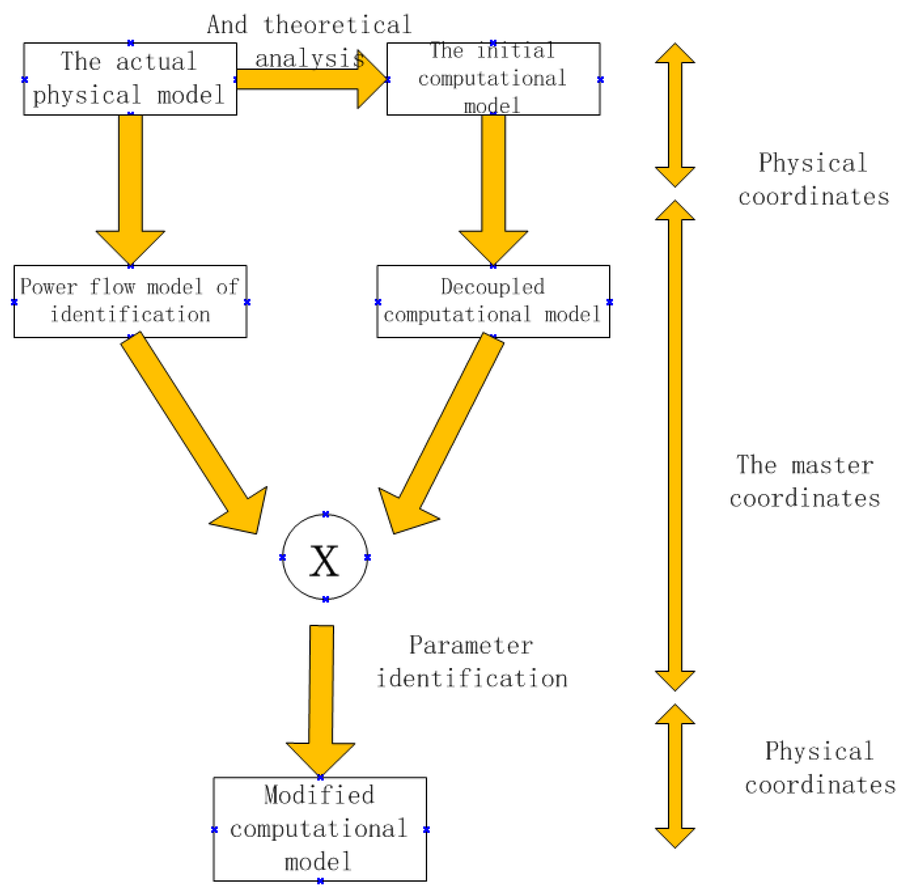
Modeling parameter identification of the hybrid FE-SEA model is related to the solution accuracy of the whole model and is the key to establishing and solving the hybrid model correctly. The identified parameters mainly include the coupling loss factor, the internal loss factor, the output power, the modal density, etc. The basic process of parameter identification is shown in Figure 1. The principle is to compare the differences between the physical model and the computational model and to realize parameter identification by comparing the decoupling model and the power-flow model. At present, there are many studies in the literature on parameter identification of the classical SEA model but few studies on parameter identification of the hybrid model. The research mainly includes the following aspects. Zhang [1] has improved the hybrid FE-SEA modeling technology. The complex dynamic system is divided into two parts to solve the problem, and the relationship between the direct field and the reverberation field is deduced. The reciprocity principle of “direct field” and “reverberation field” is applied to extend the boundary connection to any degree of freedom. At the same time, the parameter identification of the coupling loss factor of the complex system is systematically expounded. Yan [2] studied the modeling parameter identification method of the mixed FE-SEA model. The coupling loss factor, the internal loss factor, and modal density parameter identification methods are included. It is proposed that the above parameters can be solved by the FEA model, and the effectiveness of this method is verified by experiments. This method can consider the detailed structures of complex subsystems, which is helpful to improve the prediction accuracy of the hybrid FE-SEA model in the low- and medium-frequency range. The results show that the coupling loss factor of the mixed model can be obtained by using the FEA finite-element model for low- and medium-frequency analysis. Vincent Cotoni [3] pointed out that the calculation method of the reference solution in parameter identification of the mixed FE-SEA model could be verified by the finite-element random sampling method. The power-flow balance equations of the subsystems are derived by examples, and the responses of each subsystem are obtained using the power-flow balance equations. The results show that the finite-element random sampling method has a good agreement with the prediction results of the existing analysis methods. Chen [4] derived the theoretical calculation formula of the coupling loss factor for arbitrary curve connection and other connection modes according to the calculation theory of coupling loss factors for mixed-model “line connection”. The theory of parameter identification of the mixed FE-SEA model has been promoted. However, for the theoretical calculation of complex coupling systems, some problems have not been solved yet. Wu [5,6] used the interval method of Chebyshev polynomials to identify the parameters of a mixed model. The advantage of this identification method is that it does not need to determine the parameter probability distribution. It only needs to determine the parameter interval range and obtain the parameter interval of the system by solving the parameter equation. However, it is only applicable to cases in which the parameter range is small, and the error of solving the parameters in a wide range is large. To solve this problem, Wang [7] proposed an improved parameter perturbation algorithm. The method is applied to parameter identification and system-response prediction of the hybrid model. The improved parameter perturbation method preserves the higher-order term and is used to calculate the inverse of the interval matrix. The Taylor-series-correction algorithm is used to approximate the interval matrix vector, and the differences between the Monte Carlo simulation method and the parameter perturbation method are compared by examples. Zhang [8] proposed a finite-element and distribution method to solve the interval parameter linear equation of the system, which separated the non-deterministic parameters. The boundary of each parameter is determined by calculating the extremum problem of the solution of the equation. Su [9] proposed an unknown-parameter inverse analysis method. The effects of different test precisions and different target parameters on parameter identification results are compared and the convergence conditions of parameter solutions are derived. Methods for the interval parameter identification of mixed models also include the interval Gaussian elimination method, the interval iteration method, the non-probability interval method, the interval correspondence method, the interval perturbation finite-element method, and the Legendre orthogonal polynomial method [10,11,12,13,14,15,16,17].
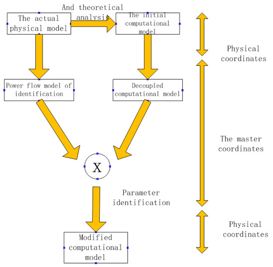
Figure 1.
Parameter identification model.
In terms of domestic research, He [18] applied the FE-SEA hybrid method to analyze the acoustic coupling problem of thin plates under the action of damping materials. Based on the SEA method, the power-flow balance equation of two subsystems is derived. The identification method of the loss-factor parameters in the thin-plate subsystem and its influence on the energy transfer of the hybrid model were studied. The FE-SEA hybrid model was established to verify the validity of parameter identification. In terms of the experimental acquisition of mixed-model parameters, Ye [19] used the PIM power input method to study the coupling loss-factor problem of the experimental acquisition of mixed-model parameters. A new method combining a theoretical method with an experimental method was proposed to determine the energy and equivalent mass of subsystems. Thus, the coupling loss factor of the system was obtained, and the influence of the test error source was avoided.
2. Basic Theoretical Parameters of the FE-SEA Method
2.1. Modal Density
In the mixed FE-SEA model, the three basic parameters required by the model are modal density, the internal loss factor, and the coupling loss factor between different subsystems. Within the research frequency range, the modal density is one of the important parameters of the subsystem, which represents the energy-storage capacity of the subsystem.
2.1.1. Lateral Vibration Modal Density of a One-Dimensional Beam
Modeling of one-dimensional elements is often encountered in mixed models. In the process of modeling, the transverse vibration of a one-dimensional beam is applied more often, and its free-state vibration equation is [1,2]:
where is the displacement of point x, R is the radius of rotation at point x, is the longitudinal wave velocity, and:
In the above formula, E is the elastic modulus of the material and is the material density. In Equation (1), ; thus, the equation can be rewritten as:
In the above formula, is the number of bending waves, and:
In the above equation, is the bending wave velocity; the modal density of the transverse vibrating beam is expressed as:
2.1.2. Modal Density of Two-Dimensional Plates
Thin-plate modeling is often used in hybrid-model modeling. For a two-dimensional flat plate, the modal density is expressed as [4]:
In the above formula, A is the total area of the thin plate, R is the radius of the bending rotation, is the two-dimensional longitudinal wave number of the flat plate, E is the elastic modulus of the corresponding flat plate, is the density of the corresponding material, and is the Poisson’s ratio of the corresponding material. For a curved plate, the empirical formulae for modal density are as follows [3,4,5]:
- (1)
- When the system frequency ratio meets the condition :
- (2)
- When the system frequency ratio meets the condition :
- (3)
- When the system frequency ratio meets the condition :
In Equations (9)–(11), F is the center frequency of the 1/3 octave, is the frequency, and F is the frequency factor. In the 1/3 octave, F = 1.122, and:
In the above formula, represents the upper-limit frequency of each frequency band of the 1/3 octave, and is the lower-limit frequency of each frequency band corresponding to it. According to the above equation, a common feature of the modal density of flat and curved plates can be obtained, that is, the modal density does not change with frequency.
2.1.3. Sound Mode Density
In the process of hybrid modeling, the sound cavity is an essential subsystem. The significance of the existence of the sound cavity lies in the surface coupling with a deterministic subsystem or a random subsystem to form the necessary connection of the hybrid model. The mode number of the sound cavity system can be expressed by the wave number of the bending wave in the sound field:
Then, the modal density of the sound cavity can be obtained by the following formula:
If the surface area of the acoustic cavity and the edge-correction term are taken into consideration, the above equation can be rewritten as:
In the above formula, is the volume of the sound field, c is the speed of sound, is the surface area of the sound field, and is the total length of all edges of the sound field.
2.2. Internal Loss Factor
2.2.1. Internal Loss Factor of the Structure
The internal loss factor of the structure is used to represent the ratio of the energy loss per unit time of each subsystem to the average energy within the unit frequency interval. In general, the internal loss factor of the structure consists of three basic components, as follows:
where is the loss factor of the structure, which is generated by the internal friction of the structure; is the loss factor generated by the “acoustic-vibration radiation” of the structure; and is the loss factor generated by the damping at the boundary junction. follows the change function of the material characteristics of the structure. is generated by the outward radiation of the vibration of the structural subsystem. The acoustic-radiation loss factor in the light-weight plate contributes more to the internal loss factor of the plate. The acoustic-radiation loss factor is a function of frequency f, and the relationship is as follows:
where is the air density, c is the sound velocity, is the radiation ratio of the subsystem, and is the area mass density of the subsystem. The calculation formula is as follows:
2.2.2. Intracavitary Loss Factor
The internal loss factor of the sound cavity can generally be obtained by measuring the average sound-absorption coefficient of the sound field. For a closed cavity, the internal sound field is a reverberation sound field formed by wave reflection. The average absorption coefficient of the whole sound cavity can be calculated by the sound-absorption coefficient on the surface of each sound cavity, and the expression is:
where is the area of the surface N of the sound cavity and is the sound-absorption coefficient of the surface N. The sound-absorption coefficient is expressed by reverberation time, and its empirical formula can be expressed as:
The time required for attenuation of 60 dB(A) in the sound cavity can be obtained. By measuring the reverberation time, the sound-absorption coefficient of the sound cavity can be obtained by the following formula:
2.3. Coupling Loss Factor
2.3.1. Coupling Loss Factor between Structures
The coupling loss factor between structures represents the strength of coupling between different subsystems and represents the energy loss generated when energy is transferred in each subsystem. All subsystems transfer energy through the coupling effect of the system. When one subsystem is excited by the external system, the energy of the subsystem is transferred to the other subsystem through the coupling effect so as to achieve energy transfer and balance. The coupling effect of different subsystems is mainly investigated via the following methods: surface connection, point connection, and line connection. There is a wire connection mode between different thin plates, and the coupling loss factor can be expressed as:
where 𝑙 is the plate connection between the curve length, represents the velocity of the bending wave of the excitation plate, represents the area of the subsystem j, represents the center frequency of the research frequency band, and represents the propagation coefficient of sound waves when they are transmitted from subsystem j to subsystem k.
2.3.2. Coupling Loss Factor between Sound Cavity and Structure
When the system is coupled with the structure for sound cavity, the coupling loss factor of the system can be expressed as:
where represents the mass density of the sound cavity subsystem, represents the sound velocity in the sound cavity, represents the mass density of the structural subsystem, and represents the sound-radiation coefficient of the structural subsystem.
2.3.3. Coupling Loss Factor between Cavity and Cavity
If the coupling connection of the system exists between two cavities, there are two ways of general connection: one is the direct connection between the cavity and the cavity, and the other is the indirect connection between the cavity and the cavity. Direct connection means that there is no other partition between subsystem j and subsystem k, and indirect connection means that there is a partition subsystem p between subsystem j and subsystem k. If there is a partition subsystem P between the sound cavity subsystem J and the sound cavity subsystem K, then the calculation formula of the coupling loss factor between them is as follows:
where is the speed of sound-wave propagation in the sound cavity, is the coupling area at the junction, is the volume of the cavity subsystem j, is the circular frequency, and is the transfer coefficient of the cavity subsystem j and the cavity subsystem k. When the two subsystems are directly connected, then in the above formula.
3. Hybrid FE-SEA Modeling Parameter Identification Algorithm
3.1. Deterministic Subsystem Response Derivation of Three-Coupled Systems
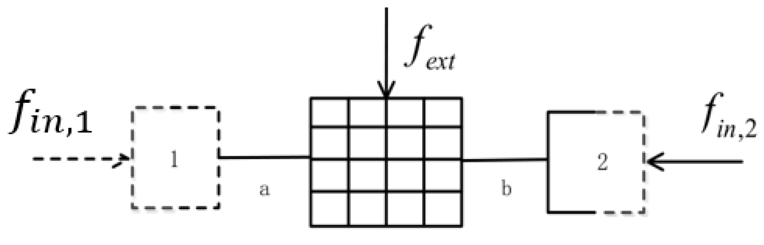
Figure 2 is a schematic diagram of the three-coupled system. It consists of a deterministic subsystem and a stochastic subsystem. In the figure, components 1 and 2 represent the random subsystem. The middle grid represents the deterministic subsystem, the dashed line represents the random boundary, the thick solid line represents the deterministic boundary, and the line segments a and b represent the hybrid connection of the two. represents the force applied to the deterministic subsystem, and represents the force applied to the random subsystem.
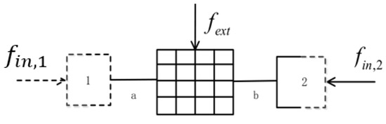
Figure 2.
Diagram of coupling between subsystems.
In the model, the number of random subsystems is N = 2, and is the reverberation field force received by the random subsystem (k = 2). represents the excitation force of the external load on the deterministic subsystem and the frequency of the force is , q represents the degree of freedom of response of the deterministic subsystem after excitation, and represents the dynamic stiffness matrix of the deterministic subsystem. Then, the motion equation of the deterministic subsystem of the three-coupled system is as follows [6,7,8]:
In the three-coupled system, is the dynamic stiffness matrix of the deterministic subsystem. The superposition of the matrix and the dynamic stiffness matrix () of the other random subsystems on the coupling boundary can be expressed as:
In general, is obtained by the finite-element method and is obtained by the boundary-element method or the analytic method. The reverberation field force needs to be confirmed before solving the displacement response of the hybrid model. Therefore, the reverberation field force () can be obtained through the reciprocal relationship between the diffusion field and the reverberation field:
where represents the population average of the system energy, represents the modal density of the random subsystem (k = 2), and represents the energy response of the random subsystem (k = 2). Therefore, a relationship is established between the deterministic subsystem and the random subsystem, which can be obtained from Equation (26):
where the output displacement q of the deterministic subsystem can be expressed in the form of a cross spectrum:
where represents the solution of the conjugate matrix after the transposition of the matrix and then the inverse of the conjugate matrix. According to the hypothesis of maximum entropy value, the interaction between the random subsystems is small and can be ignored. Then, Equation (30) can be rewritten as:
where Equation (28) is substituted into Equation (31) to obtain the displacement response of the deterministic subsystem of the three-coupled system in cross-spectral form:
Equation (32) relates the displacement cross-spectral response of the deterministic subsystem in the three-coupled system to the energy density of the random subsystem, and the motion response of the deterministic subsystem in the hybrid FE-SEA method can be obtained. In turn, the deterministic subsystem response model of multiple systems can be derived. In the process of solving the motion response of a deterministic subsystem in a coupled system, the following matters should be noted:
- (1)
- The displacement response of the deterministic subsystem obtained by this method is based on the overall average response, and the response of a certain position cannot be predicted.
- (2)
- One of the derivation conditions of the equation is that the random subsystems in the system conform to the reciprocity relation of the diffusion field, and the interaction between the random subsystems can be ignored.
- (3)
- The premise of formula derivation is the energy density () of the random subsystem, so whether the prediction of the deterministic subsystem response cross spectrum () is accurate is affected by the accuracy of the random subsystem K energy response ().
3.2. Derivation of the Energy Response of Random Subsystems of Three-Coupled Systems
3.2.1. Random Subsystem Energy Response of Three-Coupled Systems
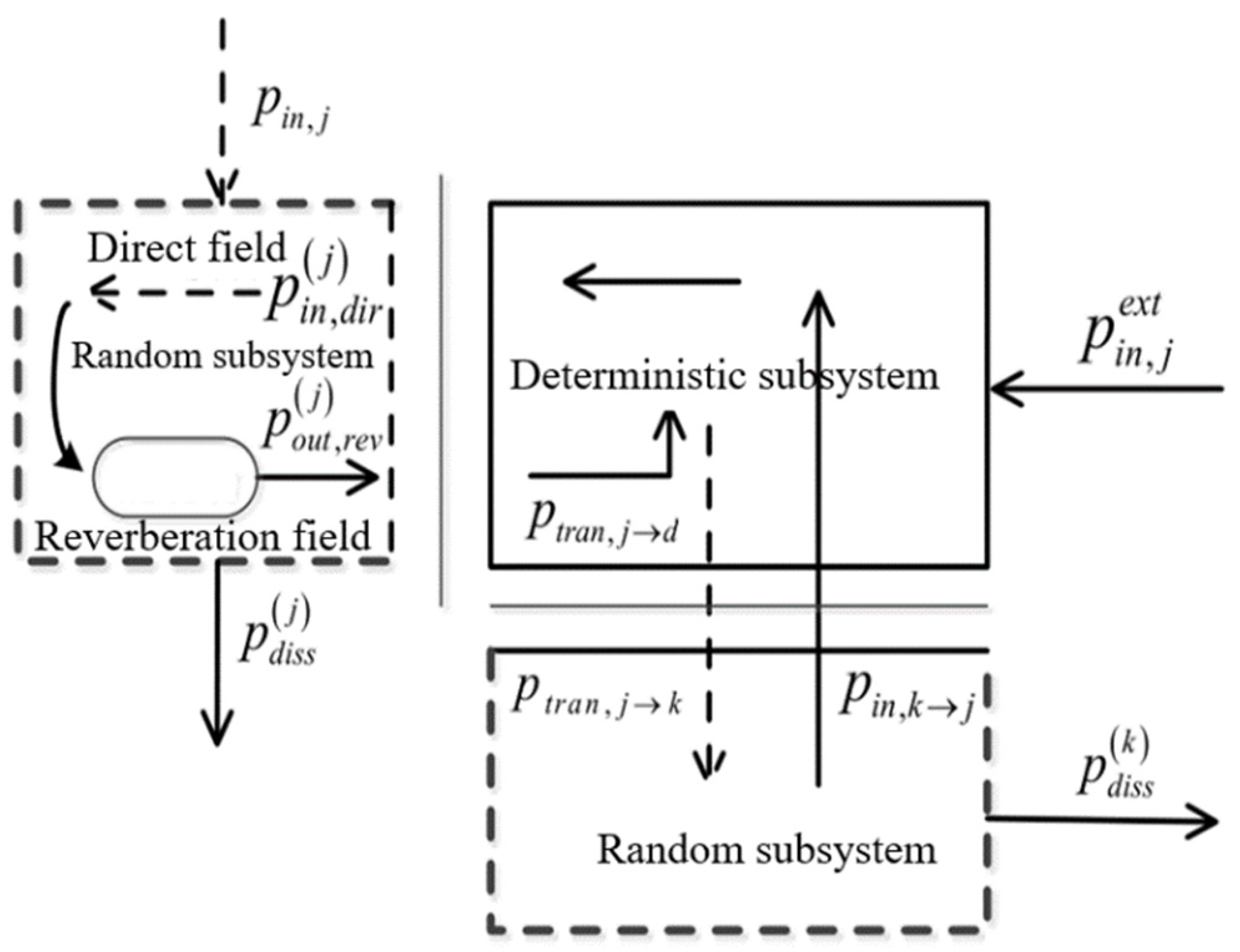
The power-flow model of the three-coupled system is shown in Figure 3. The external input power of the random subsystem is taken into account, and the power flow between the random subsystem is ignored. In the figure, the solid line represents the deterministic boundary, while the dashed line represents the random boundary. The random subsystem j (j = 1, K = 2) satisfies the following equation:
where represents the average direct field power received by the random subsystem j = 1, represents the direct input power received by the random subsystem j = 1, represents the output power of the reverberation field to the random subsystem j = 1, and represents the power consumed by the random subsystem j = 1. By expanding the above Equation (29), the displacement response of the deterministic subsystem is composed of two parts. One part is the response generated by excitation, and the other part is the response generated by the reverberation field excitation of the other random subsystems. Then, the displacement response q is expressed as [9]:

Figure 3.
FE-SEA subsystem power balance.
The direct field power flow received by a random subsystem (j = 1) is expressed as:
where r and s represent the degrees of freedom of a random subsystem (j = 1) at a deterministic boundary. Substitute Equation (34) into Equation (37):
where the first term on the right of the equation is the power of the excitation force of the deterministic subsystem acting on the system. The second term on the right of the equation is the power of the reverberation load on the system generated by other random subsystems. The two terms are unrelated, and the right-hand side of the equation is expressed as [20,21]:
Substitute Equation (39) and Equation (40) into Equation (38); then:
The power dissipation () of the subsystem (j = 1) consists of two parts. Part of the lost power is transmitted to the deterministic subsystem (d) through the reverberation field of the random subsystem (j). The other part of power loss () is transferred to other random subsystems, and it can be concluded that:
where the first part of the right side of the equation can be further expressed as:
Through Equations (35) and (36), it can be concluded that:
Substituting Equation (44) into Equation (43), the transmitted power of the random subsystem (j = 1) can be deduced:
By comparing Equation (41), the second expression on the right of Equation (42) can be deduced as follows:
Substitute Equation (45) and Equation (46) into Equation (43) to obtain the power loss of the subsystem (j = 1) in the reverberation field. According to the classical SEA method, the power consumed by the random subsystem (j = 1) is:
According to the energy-flow balance equation of the subsystem (j = 1), Equations (40), (45) and (47) are expressed as follows [22]:
In the above three formulas, there is the following relationship:
In the three-coupled system model, stands for “effective coupling loss factor” and represents the loss factor generated by the coupling between the deterministic subsystem and the random subsystem in the reverberation field. Then, the energy flow equation of the random subsystem (j = 1) is deduced as follows:
3.2.2. Energy Response of Multiple Coupled Random Subsystems Considering Power Flow
In engineering practice, the power flow of stochastic subsystem 2 and stochastic subsystem 1 is generally not negligible. A three-coupled hybrid model considering power flow is shown in Figure 4.
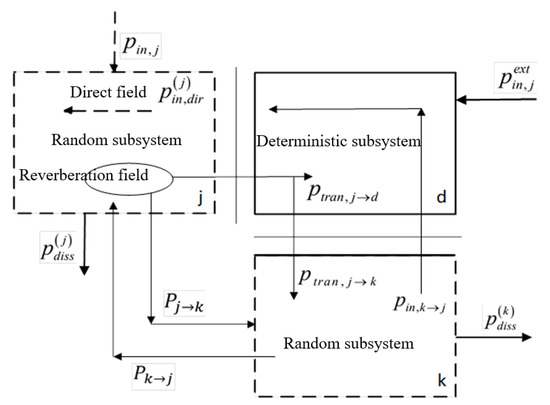
Figure 4.
Power balance of FE-SEA subsystem under power-flow conditions.
In a three-coupled system, the power-flow relationship between the random subsystems can be expressed as:
where is the input power of subsystem 2, is the power transmitted from subsystem 1 to subsystem 2, is the power transmitted from subsystem 2 to subsystem 1, and and are the power lost from subsystem 1 and subsystem 2, respectively. The following relationship is satisfied:
In the above equation, and are coupling loss factors in the classical SEA theory. Such factors are different from the effective coupling loss factor and can be obtained by combination with the energy-balance Equation (54):
Equation (61) can be rewritten as:
3.3. Derivation of Energy Response of a Random Subsystem in a Multi-Coupled System
The energy flow equation of the stochastic substructure of the three-coupled system is extended to N stochastic subsystems, and the following equation is obtained [22]:
According to the reciprocity principle of the direct field and the reverberation field, the energy-flow equation of the system can be obtained as follows:
The coupling matrix of the multi-coupled system is deduced as follows:
The coupling matrix of the system is obtained by further sorting out Equation (68):
where is the loss factor in the random subsystem, is the loss factor caused by the coupling of the deterministic subsystem and the random subsystem (j) in the reverberation field, is the coupling loss factor when two random subsystems are directly coupled, is the coupling loss factor of two stochastic and deterministic subsystems coupled together, and is the combined coupling loss factor of two random subsystems. Then, the power-balance equation of multiple systems can be deduced as follows:
3.4. Coupling Matrix Solution of the Multi-System Coupling Model
The power-balance equation of the mixed FE-SEA system can be expressed as:
Let the external excitation of the deterministic subsystem be 0, that is,. Exciting each random subsystem in turn, the power-balance equation can be obtained as follows:
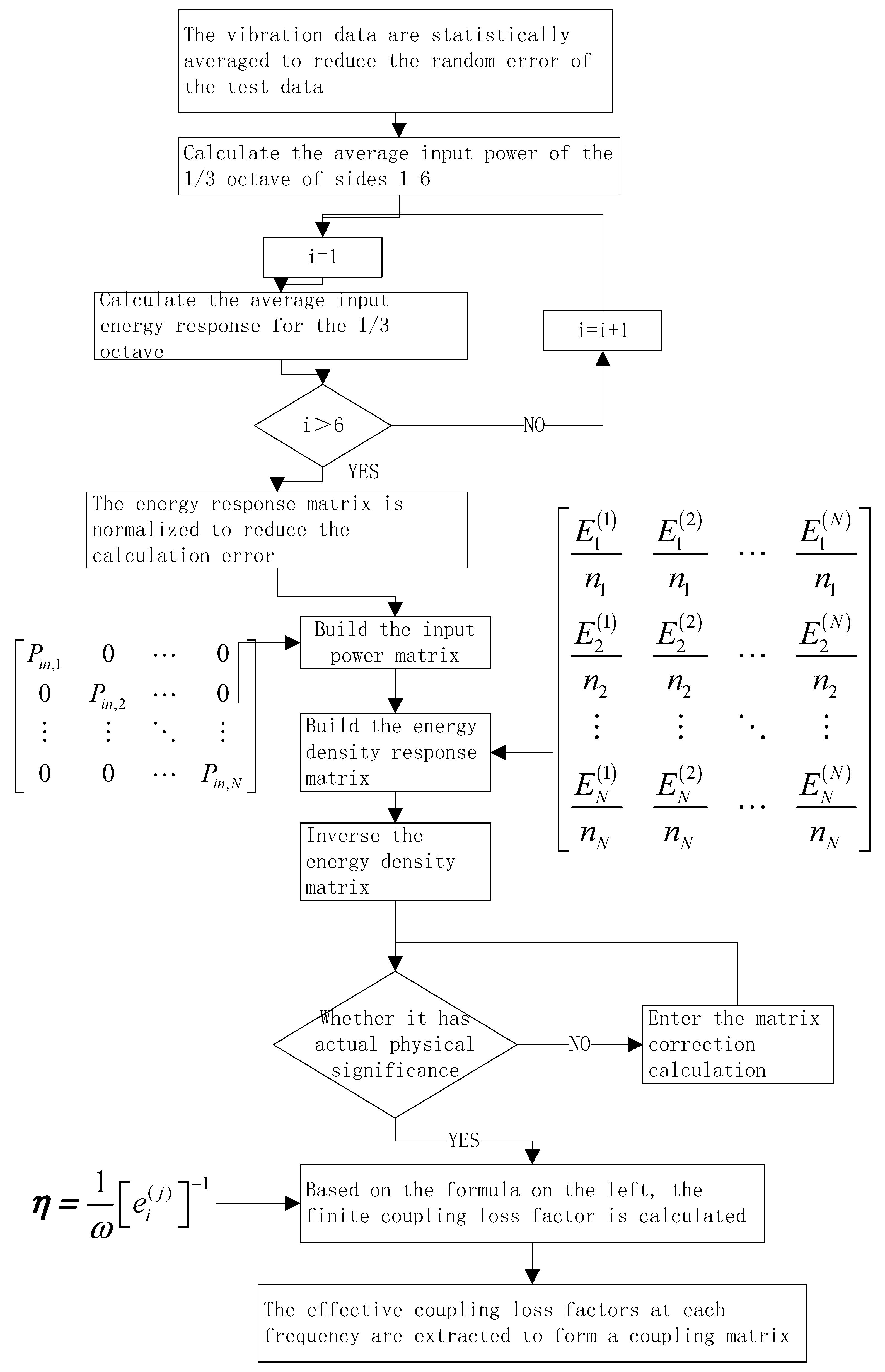
where ω is the center frequency and N represents the number of random subsystems, represents the internal loss factor of the random subsystem, and represents the loss factor caused by the coupling between the deterministic subsystem and the reverberation sound field of the random subsystem j. represents the combined coupling loss factor of two random subsystems. is the response energy of the Kth subsystem when the Jth subsystem has power input. represents the modal density of the random subsystem K. is the input power of the Jth subsystem; then, the loss-factor matrix can be obtained by inverting the energy matrix:
For the loss factor of the complex-structure system with multiple subsystems, the input power is normalized by the subsystem energy, and then the normalized modal energy can be obtained:
Therefore, Equation (72) is transformed into:
The loss-factor matrix of each subsystem can be obtained by inverting the normalized modal energy matrix:
The above algorithm designed to identify the coupling loss factor of the mixed FE-SEA model can be realized by MATLAB. The flow chart of this algorithm is shown in Figure 5.
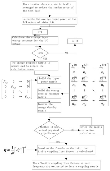
Figure 5.
Matlab process of hybrid FE-SEA model coupling loss-factor algorithm.
3.5. Iterative Improvement of Ill-Conditioned Matrix Parameters
In general, the energy matrix will appear as an ill-conditioned matrix. Parameter iteration is carried out for the ill-conditioned matrix, and parameter correction of the energy matrix is realized. Assume that the general representation of the energy matrix is as follows [11]:
where A is the coefficient matrix, B is the diagonal matrix, and x is the solution vector. If is the weighting factor and E is the identity matrix of order n, then is added to the left and right ends of Equation (77) according to the principal-component weighting method to obtain:
In general, the ill-conditioned matrix of a system of linear equations is measured according to the number of conditions. The condition number of the coefficient matrix (A) is related to the ill-condition degree of the linear equations. For matrix A, when the weighting factor α > 0, the following relation holds (Cond (A+ αe) < Cond (A)), where cond represents the number of conditions. By transforming Equation (77) into Equation (78), the number of conditions of the equation is reduced, and the ill-condition degree of the linear equations can be reduced. Since the left and right sides of Equation (78) contain a solution x, the iterative relationship can be constructed as follows:
If , then:
If is small enough, when , approximate solutions can be found, where and are the solutions obtained after iterating (k) times and iterating (k + 1) times, respectively. and represent the norms of and , respectively. is a constant term of a smaller order of magnitude.
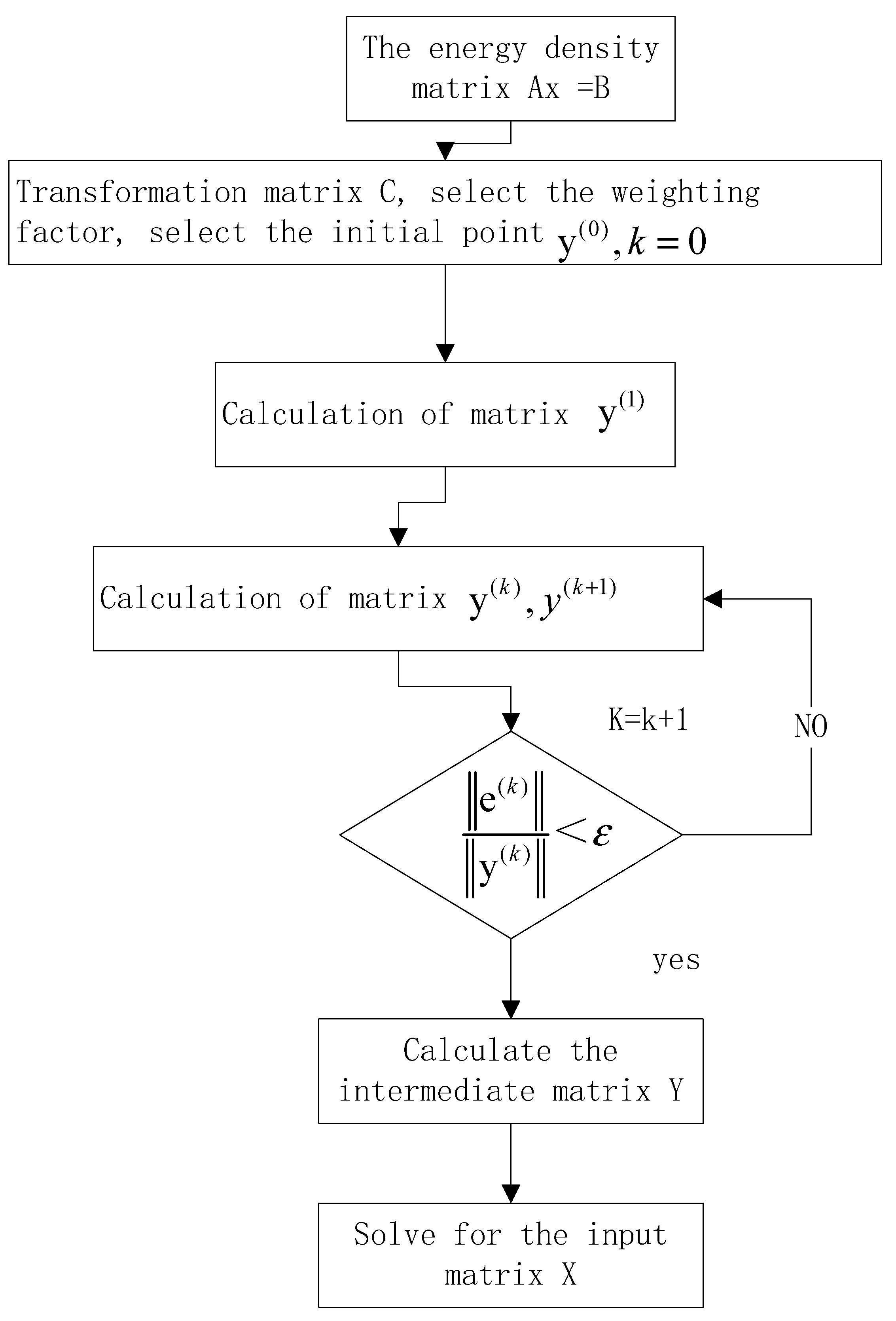
In order to improve the accuracy and stability of the calculation results, an error-correction method is introduced based on the principal-component-weighted iterative method. A new ill-conditioned matrix iteration method is presented. In general, the ill-conditioned matrix equation is solved directly. The solution x appears easily in the ill-conditioned matrix, and the calculation error is large. When performing the calculation, enter matrix C first and rewrite Equation (77) as:
where matrix C is an N × N nonsingular matrix. The vector y is solved according to Equation (83). The error can be corrected by Equation (84) to obtain a solution with less error.
The error is transferred to the intermediate variable y by Equation (84) to avoid solving x. Improve the accuracy of solving x. Then, add the variable αx to both sides of the transformed matrix Equation (83) to obtain:
According to the iterative formula, the relationship is as follows:
The matrix Equation (86) is solved to obtain the intermediate variable y. Finally, the exact solution x is obtained through Equation (84). The ill-conditioned matrix parameter iteration method combines the error-correction shift with the principal-component-weighted iteration method. It improves the traditional principal-component-weighted iterative method. Firstly, the matrix solution set X is converted to the matrix CY, and the weighted iterative method of principal components is used to solve ACy = B, thus obtaining the intermediate variable Y. Then, the exact solution x is obtained from the matrix x = Cy. This method can further improve the accuracy and stability of understanding. The specific steps are as follows:
- (1)
- Select matrix C and transform matrix AX = B to ACy = B.
- (2)
- Select factor α. Then, select the initial point value and use the decomposition method to solve to obtain the value of .
- (3)
- Iterate into the loop and calculate .
- (4)
- Solve .
- (5)
- Solve .
- (6)
- When , the iterative cycle ends and the solution vector y is obtained.
- (7)
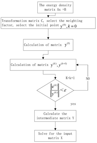 Figure 6. Iterative flow of ill-conditioned energy matrix.
3.6. The Algorithm of a Case Analysis
3.6.1. Numerical Example
According to the multi-system coupling model, a hybrid FE-SEA model of six subsystems was established, as shown in Figure 7. The hybrid model consists of six square steel plates welded together. The material parameters are shown in Table 1. The density of the steel plate was 7800 kg/m3; the Poisson’s ratio was 0.3; the elastic modulus E = 200 GPa; the length and width of the steel plate were 1000 mm and 1000 mm, respectively; the thickness was 1 mm; and the damping loss factor of the steel plate was 0.01. The analysis frequency range of the hybrid model was 0–2000 Hz, and unit-frequency excitation was performed on each plate to obtain the average vibration energy, the modal density, and the input power for each plate. The Monte Carlo calculation method was used as the reference solution to compare the effects of the mixed FE-SEA method and the improved FE-SEA method [20]. As shown in Figure 8, the test device was built according to a 1:1 ratio between the model and the real object. The effective coupling loss factor was improved and verified. The test system was composed of a physical sample, an acceleration sensor, a shaker, a rope, and a test data line. Each measuring point on the surface of the physical sample was excited separately, and the acceleration and velocity signals of each measuring point were tested. The shaker selected a sinusoidal peak force of 100 N and a frequency range of 5–10 KHz. Nine measuring points were selected for each board of the physical sample, and each measuring point was tested three times to obtain an average value. For the acceleration sensor PCB, ±50 g was selected, and the sensitivity was 100 mv/g. The acceleration and velocity of each measuring point and the force of each measuring point were measured by the power input method. The input power and energy of each measuring point were calculated according to the statistical-energy power input method.
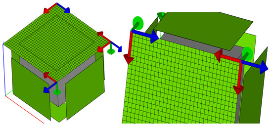
Figure 7.
FE-SEA statistical energy model.

Table 1.
Mixed-model material parameters.
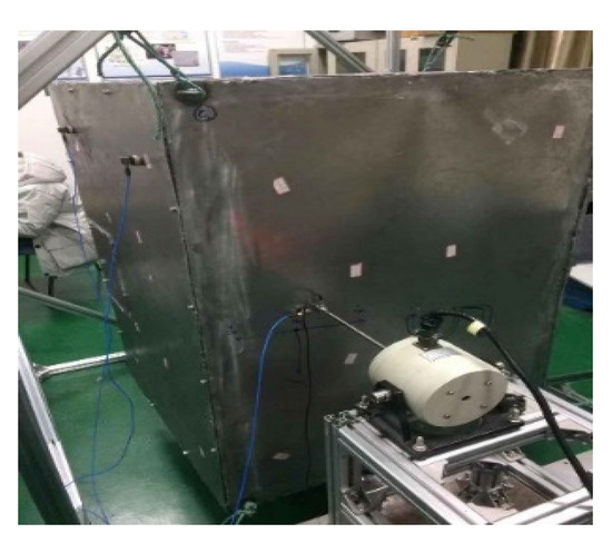
Figure 8.
Parameter test system.
3.6.2. System Response Analysis
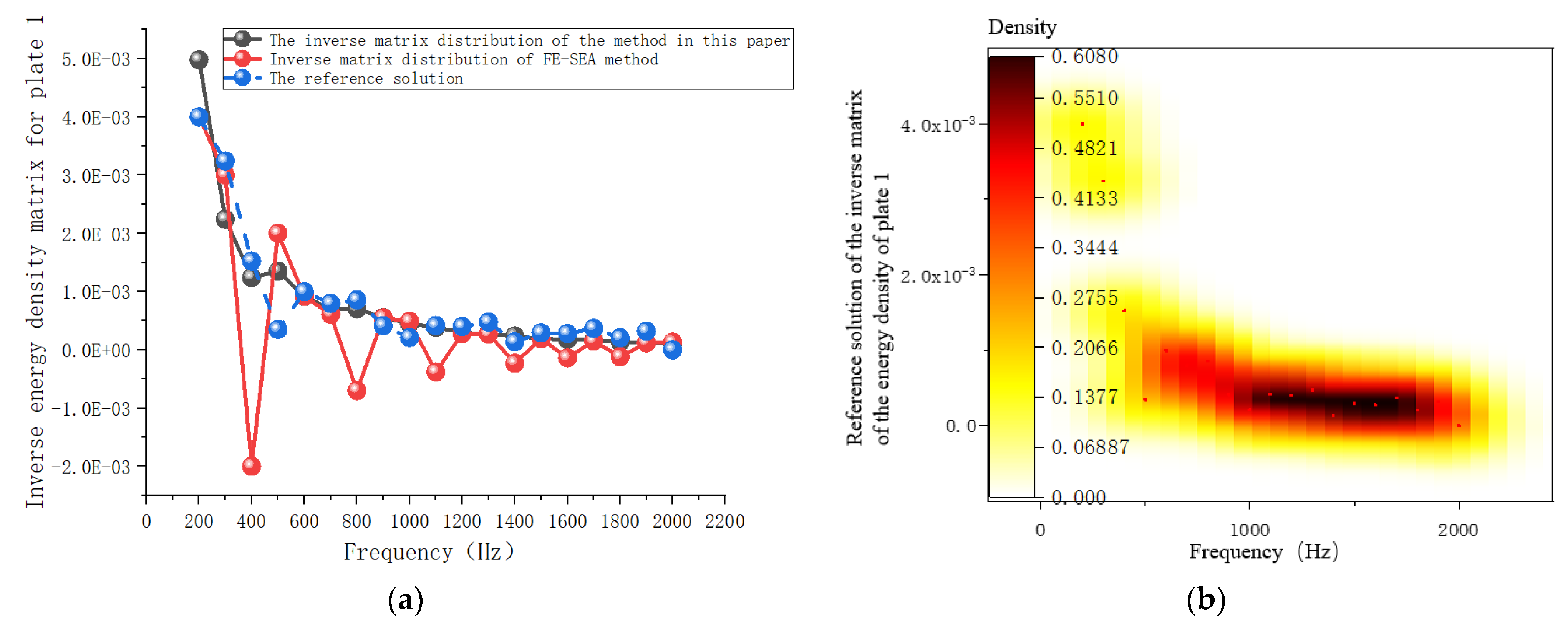
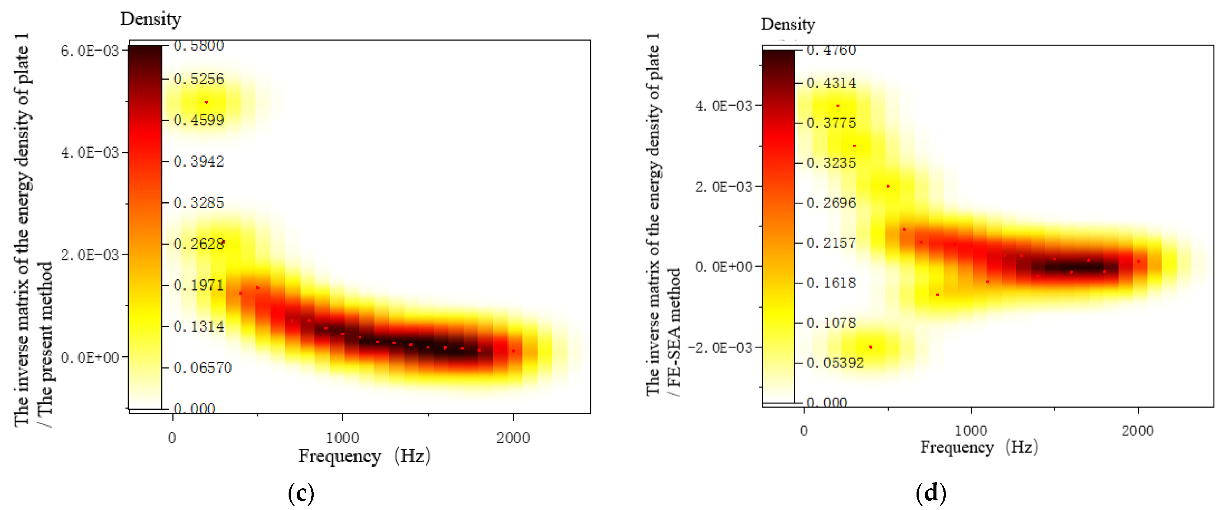
The FE-SEA hybrid method and the improved FE-SEA method were used to solve the subterms of Equation (73), and the inverse matrix results of the energy density of the subsystem are shown in Figure 9, Figure 10 and Figure 11. When plate 1 was used for the excitation, as shown in Figure 9a, an ill-posed matrix appeared when solving the inverse matrix of the energy density through the mixed FE-SEA method, and a singular value appeared when solving the inverse matrix of the energy density. The principal-element iteration of the ill-conditioned matrix parameters was carried out by the inverse operation of the energy density matrix. Thus, the above problems were solved. In the whole calculation frequency band, no ill-posed matrix appeared, and the fitting degree with respect to the reference solution was high. Figure 9b–d are the inverse matrix distributions obtained by the reference solution method, the proposed method, and the mixed FE-SEA method, respectively. It can be seen from the figure that the inverse matrix obtained by this method was reasonably distributed and had no ill-posed singular matrix values.
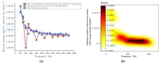
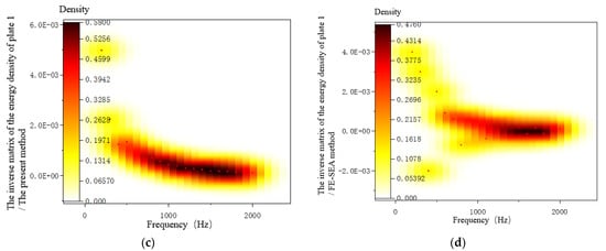
Figure 9.
The inverse matrix of the energy density of plate 1. (a) The inverse matrix of the energy density of plate 1. (b) The inverse matrix distribution of the reference solution. (c) The inverse matrix distribution of the present method. (d) The inverse matrix distribution of the FE-SEA method.
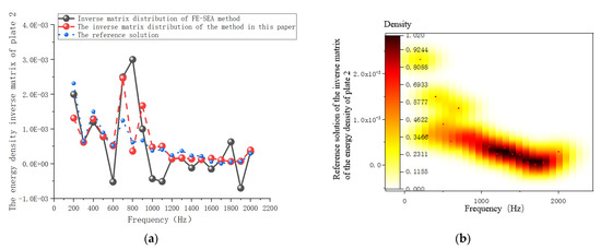

Figure 10.
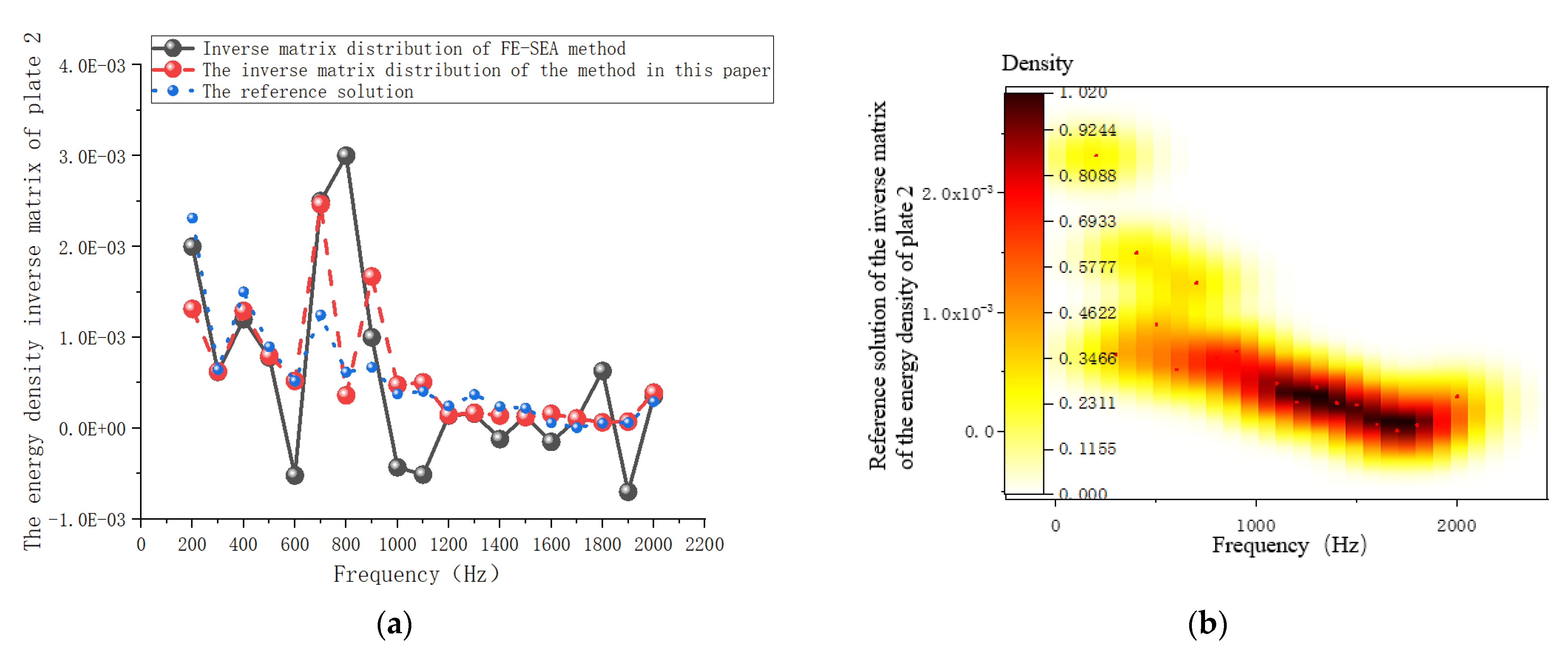
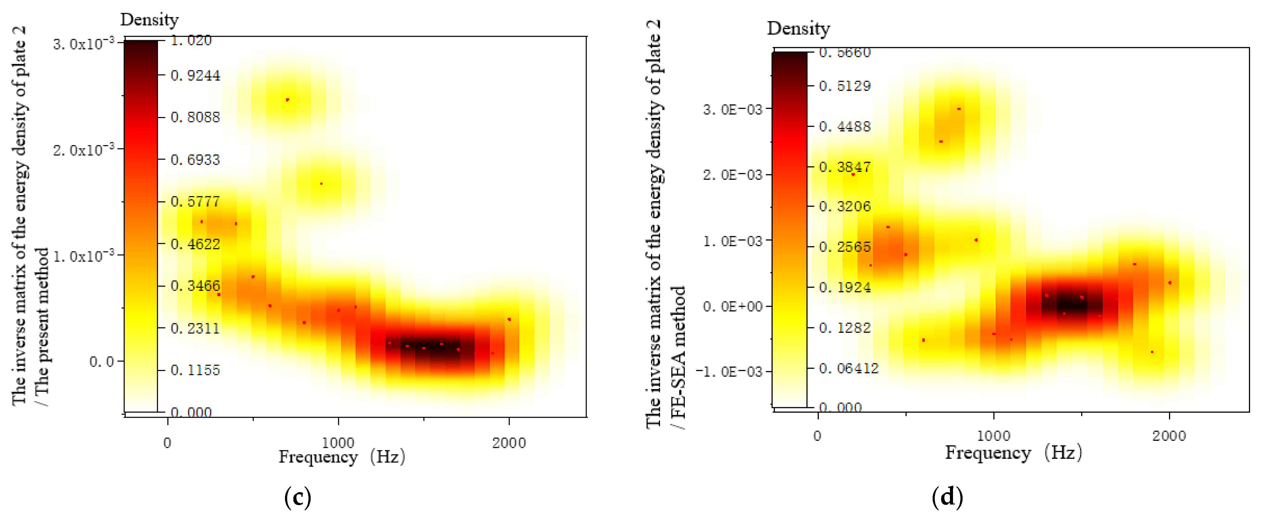
The inverse matrix of the energy density of plate 2. (a) The inverse matrix of the energy density of plate 2. (b) The inverse matrix distribution of the reference solution. (c) The inverse matrix distribution of the present method. (d) The inverse matrix distribution of the FE-SEA method.
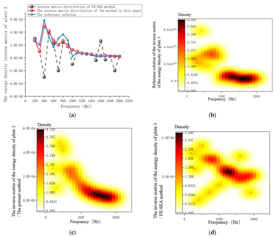
Figure 11.
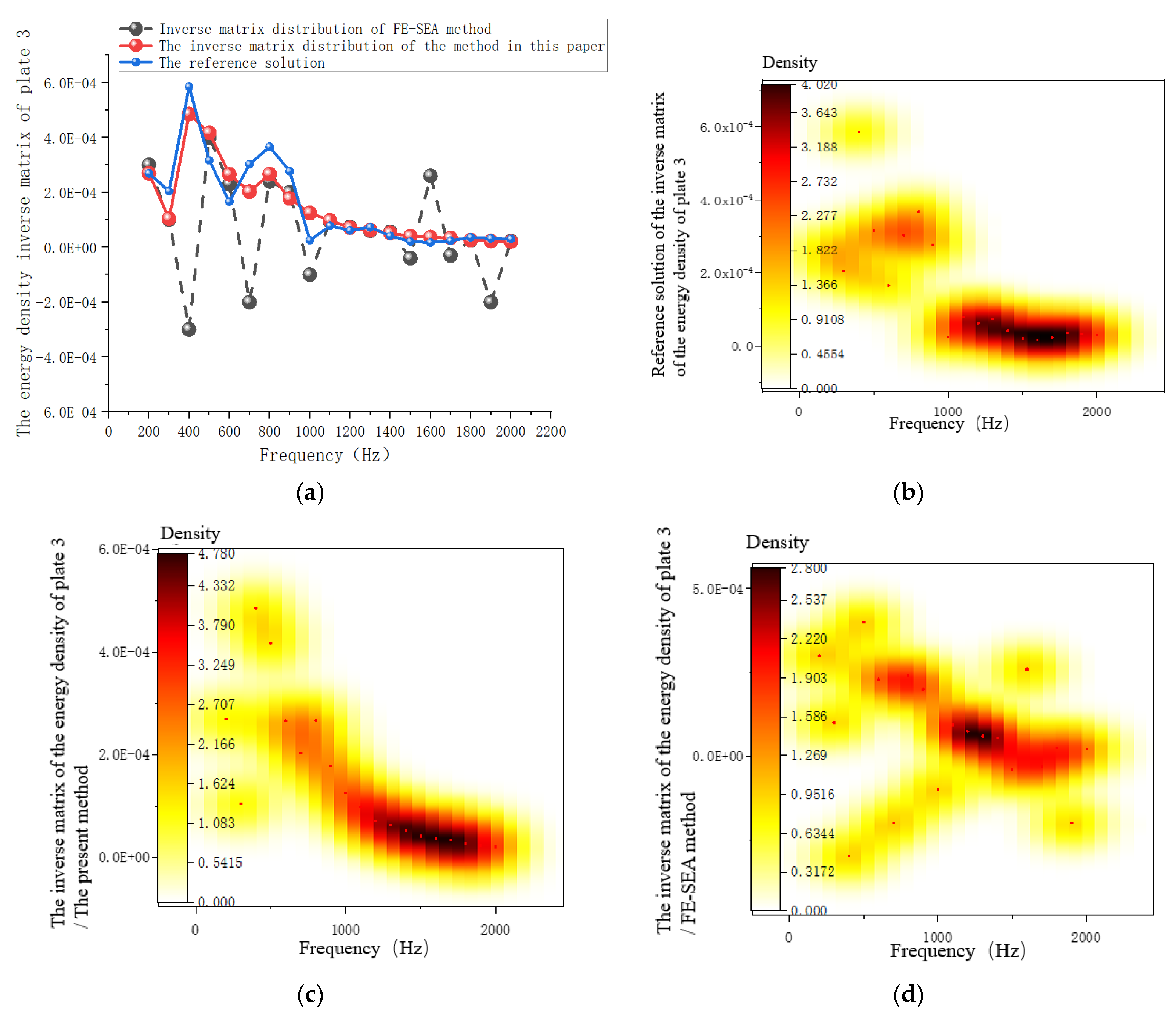
The inverse matrix of the energy ratio density of plate 3. (a) The inverse matrix of the energy density of plate 3. (b) The inverse matrix distribution of the reference solution. (c) The inverse matrix distribution of the present method. (d) The inverse matrix distribution of the FE-SEA method.
When plate 2 was used as the excitation surface, as shown in Figure 10a, the ill-posed matrix appeared when solving the inverse matrix of the energy density by the mixed FE-SEA method. Singular solutions appeared in the inverse matrix of the ratio of subsystem energy to subsystem modal density. There was no ill-posed matrix in the whole calculated frequency band, and the improved method had a high degree of fit with the reference solution. Figure 10b–d show the inverse matrix distribution obtained by the reference solution method, the proposed method, and the mixed FE-SEA method, respectively. It can be seen from the distribution results that the distribution of the inverse matrix solution obtained by the method in this paper was reasonable and that no ill-posed matrix appeared. Similarly, as shown in Figure 11, the conclusion regarding system excitation plate 3 was basically consistent with that for excitation plates 1 and 2. The parameter iteration of the ill-conditioned matrix can solve the inverse problem of energy density in the solution process of the mixed FE-SEA. Compared with reference [21], the method for solving the energy matrix of the mixed FE-SEA method was extended. The disadvantages of neglecting the inverse matrix of the energy density of the process parameters in the existing calculation methods are given. A new method for solving the hybrid model is presented which has good research significance for further solving the effective coupling loss factor of the system.
3.6.3. Coupling Loss-Factor Analysis of the System
In order to further verify the effectiveness of the improved mixed FE-SEA method, the effective coupling loss factors of each plate were compared. Figure 12 shows the results of the effective coupling loss factor transferred from plate 1 to plate 2. It can be seen from Figure 12a that plate 1 is the excitation surface, and the effective coupling loss factors calculated by the mixed FE-SEA method appear as singular solutions at individual frequency points, which are regarded as the invalid coupling matrix. In the method presented in this paper, the application of the principal-component correction method to determine the coupling matrix subsystem energy density was used to obtain the ratio of the inverse matrix and calculate the effective coupling loss factor of the effective matrix in order to effectively calculate the mixed FE—SEA model, the effective coupling loss factor of the feasible method providing a theory and the calculation results tallying with the test results. The improved hybrid FE-SEA method in the frequency range of 400–2000 Hz had a high degree of fit with the test results, which verified the effectiveness of the proposed method. Compared with the existing literature, the cumulative errors caused by the application of theoretical analytical solutions to solve the effective coupling loss factors in complex structures is avoided, and the calculation accuracy in the frequency band of 1000–2000 Hz is improved, which is more suitable for the solution of the effective coupling loss factors in complex structures [22]. Figure 12b–d are the distribution diagrams of effective coupling loss factors obtained by the test method, the mixed FE-SEA method, and the proposed method, respectively. It can be seen from the figures that the distribution of the effective coupling loss factors obtained by the proposed method is reasonable and that no invalid coupling matrix appears.
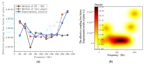
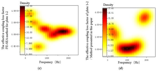
Figure 12.
Effective coupling loss factor of plates 1–2. (a) Comparison of several calculation methods of coupling loss factors. (b) Test results. (c) FE-SEA method. (d) The present method.
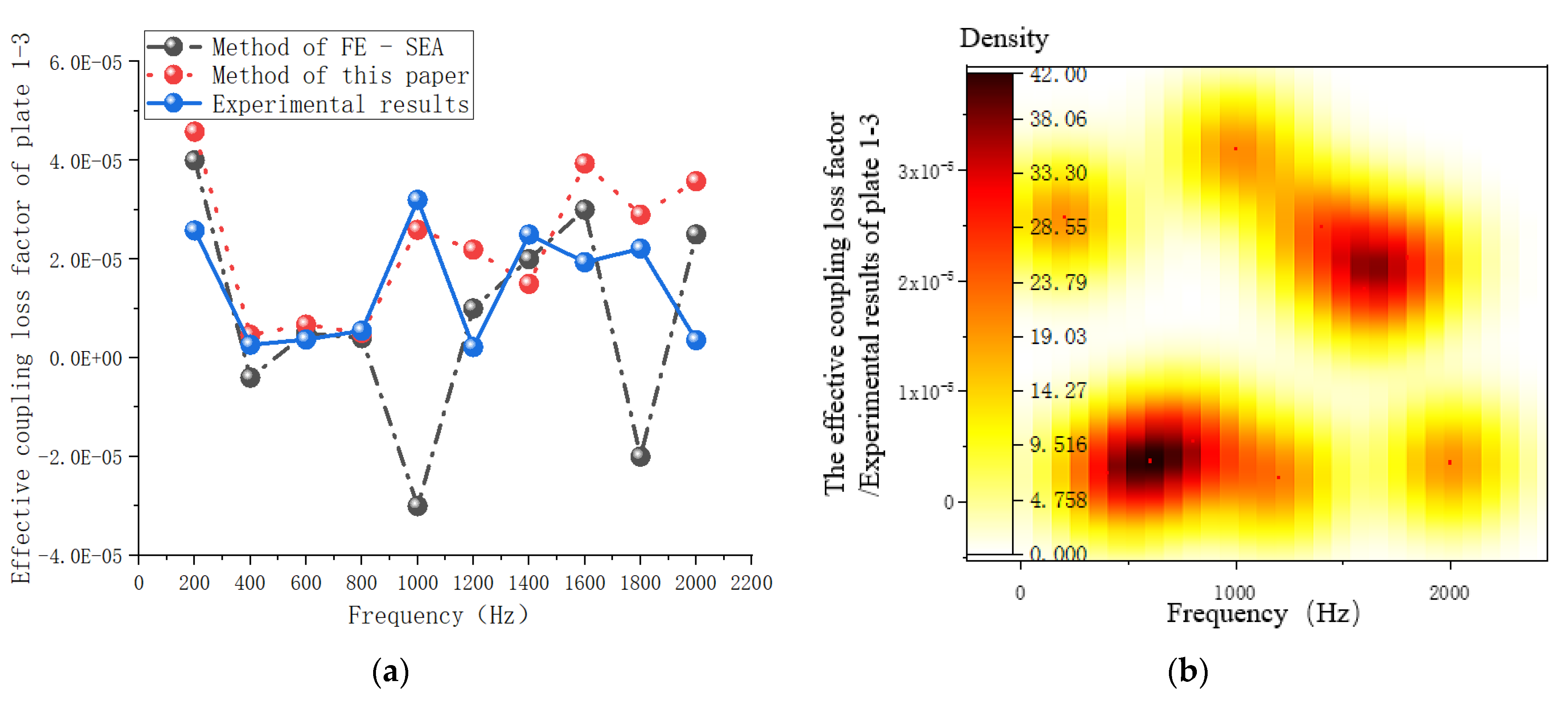
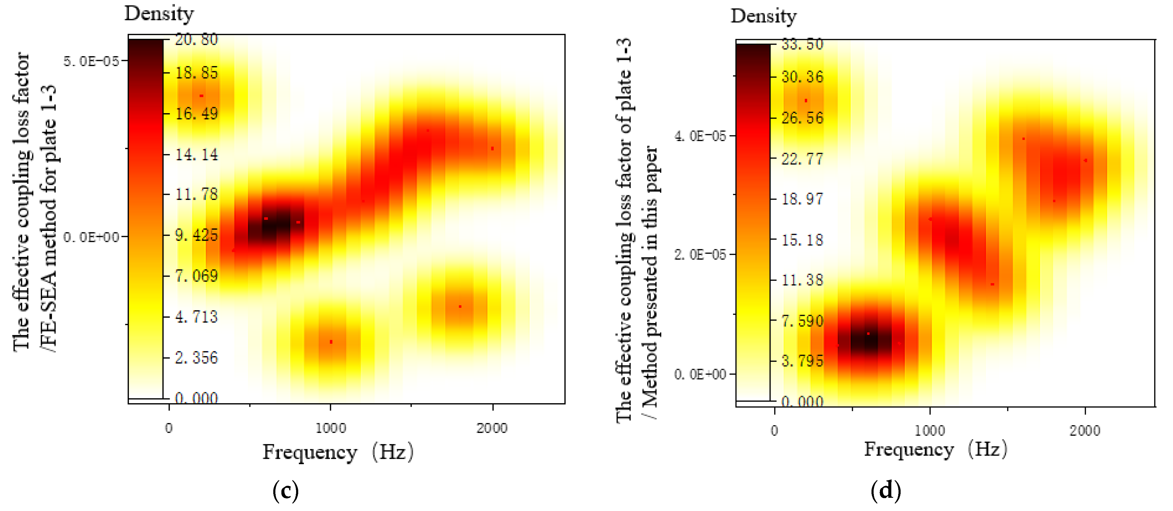
Figure 13 shows the results of the effective coupling loss factor transferred from plate 1 to plate 3. It can be seen from Figure 13a that plate 1 is the excitation surface, and the effective coupling loss factor calculated by the mixed FE-SEA method presents an invalid coupling matrix region at such frequency points as 400 Hz, 1000 Hz, and 1800 Hz. In this paper, the principal-element correction method was used to correct the inverse matrix of the ratio between the subsystem energy and the modal system, and the effective coupling loss factors calculated were all effective coupling matrices, which were in good agreement with the test results. In the frequency ranges of 0–1000 Hz and 1400–2000 Hz, the improved hybrid FE-SEA method had a high degree of fit with the test results, which verified the effectiveness of the proposed method. Figure 13b–d are the distribution diagrams of the effective coupling loss factors obtained by the test method, the mixed FE-SEA method, and the proposed method, respectively. It can be seen from the figures that the distribution of the effective coupling loss factors obtained by the proposed method is reasonable.


Figure 13.
Effective coupling loss factors of plates 1–3. (a) Comparison of several calculation methods of coupling loss factors. (b) Test results. (c) FE-SEA method. (d) The present method.
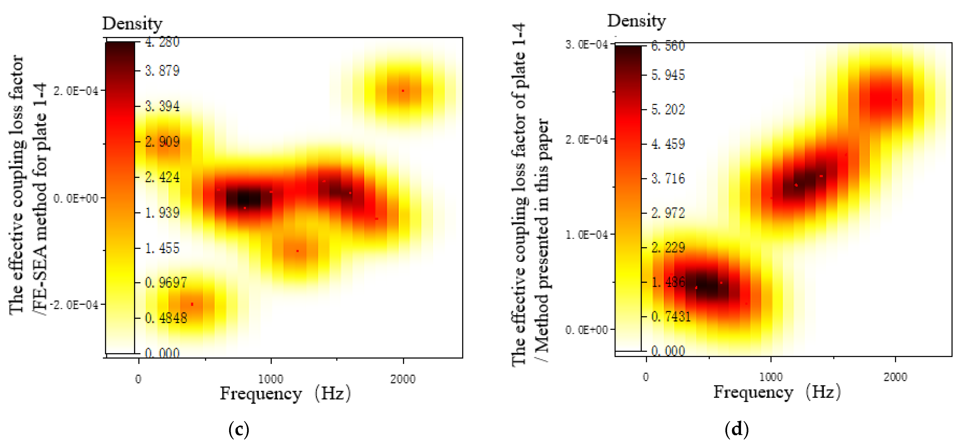
Figure 14 is the result of the effective coupling loss factor transferred from plate 1 to plate 4. It can be seen from Figure 14a that plate 1 was used as the excitation surface, and the hybrid FE-SEA method was used to calculate the effective coupling loss factor at such frequency points as 400 Hz, 800 Hz, 1200 Hz, and 1800 Hz, and an invalid coupling matrix region appeared. In the improved method, the principal-element correction method is used to correct the inverse matrix of the ratio of subsystem energy to subsystem model density, which solves the problem of the invalid coupling matrix mentioned above. The effective coupling loss factors calculated were all effective coupling matrices, which were in good agreement with the test results. In the frequency ranges of 0–1000 Hz and 1200–2000 Hz, the improved hybrid FE-SEA method had a high degree of fit with the test results, which verified the effectiveness of the proposed method. Figure 14b–d are the distribution diagrams of effective coupling loss factors obtained by the test method, the mixed FE-SEA method, and the proposed method, respectively. It can be seen from the figures that the distribution of the effective coupling loss factors obtained by the proposed method is reasonable.
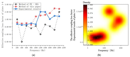
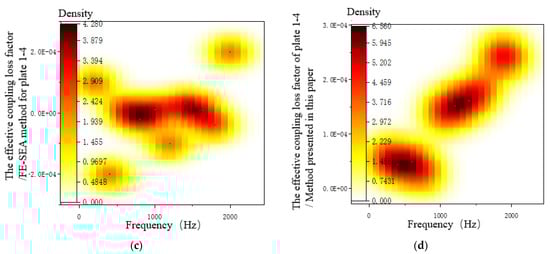
Figure 14.
Effective coupling loss factors of plates 1–4. (a) Comparison of several calculation methods of coupling loss factors. (b) Test results. (c) FE-SEA method. (d) The present method.
4. Conclusions
In this paper, the energy-flow method was adopted to establish a mixed FE-SEA model with three-coupled systems and a multi-system coupling model to solve the intermediate-frequency solving accuracy problem of the existing mixed FE-SEA model. The parameter identification of effective coupling loss factors in the mixed FE-SEA model was studied. The system response of deterministic components and the energy response of stochastic subsystems in three-coupled systems were derived. Based on the three-coupled system models, the multi-system coupling system response solution method was extended. Aiming at the ill-posed matrix problem for the solution of energy-specific density in the hybrid FE-SEA model with the existing technology, an improved principal-component-weighted correction method was applied by introducing intermediate variables and error transfer. The inverse matrix of energy density was modified to solve the singular-value problem of the ill-posed matrix. In order to further verify the effectiveness of the improved hybrid FE-SEA model parameter identification method, the calculation results of the effective coupling loss factors of each plate were compared. The results showed that the effective coupling loss factor calculated by the mixed FE-SEA method had a singular solution at some frequency points, which was an invalid coupling matrix. In this paper, the principal-element correction method was used to correct the inverse matrix of the ratio of subsystem energy to modal density in the coupling matrix. The effective coupling loss factors calculated were all effective coupling matrices. The effective coupling loss factors calculated by the improved mixed FE-SEA method at the frequency of 400–2000 Hz had a high degree of fit with the test results, which verifies the effectiveness of the proposed method. Compared with the existing literature, the cumulative error caused by the application of the theoretical analytical solution to the effective coupling loss factors in complex structures is avoided. In the calculation frequency range of 1000–2000 Hz, the calculation accuracy of the frequency band was also improved, and the overall calculation error of the whole frequency band was less than 10%, which has a certain engineering-application significance. An effective solution for calculating coupling loss factors via the mixed FE-SEA model has been provided.
Author Contributions
J.S. is responsible for the technical route of the full text. L.Z. is responsible for the full text program writing. All authors have read and agreed to the published version of the manuscript.
Funding
The research was financially supported by the Hubei Superior and Distinctive Discipline Group of “New Energy Vehicle and Smart Transportation”.
Institutional Review Board Statement
Not applicable.
Informed Consent Statement
Not applicable.
Data Availability Statement
All data are true and valid.
Conflicts of Interest
The authors declare no conflict of interest.
References
- Langley, R.S.; Bremner, P. A hybrid method for the vibration analysis of complex structural-acoustic systems. J. Acoust. Soc. Am. 1999, 105, 1657–1671. [Google Scholar] [CrossRef]
- Yan, H.H.; Parett, A.A. A FEA-Based Procedure to Perform Statistical Energy Analysis; SAE Technical Paper 2003-01-1553; SAE International: Warrendale, PA, USA, 2003. [Google Scholar]
- Cotoni, V.; Gardner, B.; Shorter, P.; Lane, S. Demonstration of Hybrid FE-SEA Analysis of Structure-Borne Noise in the Mid Frequency Range; SEA International Paper 2005-01-2331; SAE International: Warrendale, PA, USA, 2005. [Google Scholar]
- Chen, S.M.; Wang, D.F.; Zuo, A.K.; Chen, Z.; Zhao, X.M.; Zan, J.M. Calculation of coupling loss factors of several line junctions. J. Jilin Univ. 2010, 4, 920–924. [Google Scholar]
- Wu, J.L.; Zhang, Y.Q. The dynamic analysis of multibody systems with uncertain parameters using interval method. Appl. Mech. Mater. 2012, 152, 1555–1561. [Google Scholar] [CrossRef]
- Wu, J.; Luo, Z.; Zhang, Y.; Zhang, N.; Chen, L. Interval uncertain method for multibody mechanical systems using Chebyshev inclusion functions. Int. J. Numer. Methods Eng. 2013, 95, 608–630. [Google Scholar] [CrossRef]
- Wang, C.; Qiu, Z. An interval perturbation method for exterior acoustic field prediction with uncertain-but-bounded parameters. J. Fluids Struct. 2014, 49, 441–449. [Google Scholar] [CrossRef]
- Zhang, J.G. A Method for static interval analysis of uncertain structures with interval parameters. In Advanced Materials Research; Trans Tech Publications Ltd.: Stafa-Zurich, Switzerland, 2014; Volume 950. [Google Scholar]
- Su, J.B.; Liu, H.B.; De Zhao, H.; Zhang, D. Research on interval reversible inverse analysis method based on interval parameters. In Advanced Materials Research; Trans Tech Publications Ltd.: Stafa-Zurich, Switzerland, 2013; pp. 556–559. [Google Scholar]
- Reynders, E.; Langley, R.S.; Dijckmans, A.; Vermeir, G. A hybrid finite element—Statistical energy analysis approach to robust sound transmission modeling. J. Sound Vib. 2014, 333, 4621–4636. [Google Scholar] [CrossRef]
- Moens, D.; Vandepitte, D. Recent advances in non-probabilistic approaches for non-deterministic dynamic finite element analysis. Arch. Comput. Methods Eng. 2006, 13, 389–464. [Google Scholar] [CrossRef]
- Moens, D.; Hanss, M. Non-probabilistic finite element analysis for parametric uncertainty treatment in applied mechanics: Recent advances. Finite Elem. Anal. Des. 2011, 47, 4–16. [Google Scholar] [CrossRef]
- Belyaev, A.K. Dynamic simulation of high-frequency vibration of extended complex structures. J. Struct. Mech. 2007, 20, 155–168. [Google Scholar] [CrossRef]
- Rao, S.S.; Berke, L. Analysis of uncertain structural systems using interval analysis. Aiaa J. 1997, 35, 727–735. [Google Scholar] [CrossRef]
- Qiu, Z.; Chen, S.; Elishakoff, I. Bounds of eigenvalues for structures with an interval description of uncertain-but-non-random parameters. Chaos Solitons Fractals 1996, 7, 425–434. [Google Scholar] [CrossRef]
- Xu, M.; Qiu, Z.; Wang, X. Uncertainty propagation in SEA for structural–acoustic coupled systems with non-deterministic parameters. J. Sound Vib. 2014, 333, 3949–3965. [Google Scholar] [CrossRef]
- Wu, J.; Zhang, Y.; Chen, L.; Luo, Z. A Chebyshev interval method for nonlinear dynamic systems under uncertainty. Appl. Math. Model. 2013, 37, 4578–4591. [Google Scholar] [CrossRef]
- He, Y.; Zhang, H.; Xia, X.; Xu, Z.; Zhang, Z. Analysis of Noise Reduction of Car Body Panel Based on FE-SEA Hybrid Method. J. Vib. Shock 2016, 35, 234–240. [Google Scholar]
- Ye, M.; Lang, Z.G.; Hao, Z.Y. Measurement of SEA Parameters in Vibration Energy Balance Equation of Complex System. Trans. CSICE 1998, 16, 469–474. [Google Scholar]
- Zhu, W.; Xing-Rui, M.A.; Han, Z.; Zou, Y. Research on Modeling Method of Hybrid FE-SEA Wire Connection. J. Vib. Eng. 2016, 5, 17–23. [Google Scholar]
- Wu, F.; Li, G.Y.; Cheng, A.G. Analysis of Acoustic-structure Coupling of Intermediate Frequency Based on Hybrid ES-FE-SEA Method. Chin. J. Mech. Eng. 2015, 2015, 73–80. [Google Scholar]
- Chen, S.M. Research on the Prediction and Control Method of High Frequency Noise in Car. Ph.D. Thesis, Jilin University, Changchun, China, 2011. [Google Scholar]


Disclaimer/Publisher’s Note: The statements, opinions and data contained in all publications are solely those of the individual author(s) and contributor(s) and not of MDPI and/or the editor(s). MDPI and/or the editor(s) disclaim responsibility for any injury to people or property resulting from any ideas, methods, instructions or products referred to in the content. |
© 2023 by the authors. Licensee MDPI, Basel, Switzerland. This article is an open access article distributed under the terms and conditions of the Creative Commons Attribution (CC BY) license (https://creativecommons.org/licenses/by/4.0/).