A Machine Learning Approach to the Non-Invasive Estimation of Continuous Blood Pressure Using Photoplethysmography

Abstract

Blood pressure is an important vital sign that sometimes requires continuous measurement. The current methods include cuff measurements (manual auscultation and oscillometric techniques) for non-continuous measurement and invasive arterial cannulation for continuous measurement. The use of photoplethysmography as a cuffless, non-invasive, and continuous blood pressure measurement system is investigated through the use of four neural networks. These predict the systolic blood pressure, diastolic blood pressure, mean arterial blood pressure, and waveform shape. The models are trained on 890 h of data from 1669 patients in the MIMIC-III database. Feature-trained artificial neural networks predict the systolic blood pressure to 5.26 ± 6.53 mmHg (mean error ± standard deviation), the diastolic blood pressure to 2.96 ± 3.31 mmHg, and the mean arterial pressure to 3.27 ± 3.55 mmHg. These are used to shift and scale the predicted waveform, allowing the waveform prediction neural network to optimise for the wave shape rather than the amplitude. The waveform prediction has 86.4% correlation with the actual arterial blood pressure waveform. All results meet international clinical blood pressure measurement standards and could potentially change how blood pressure is measured in both clinical and research settings. However, more data from healthy individuals and analysis of the models’ biases based on clinical features is required.

1. Introduction

One of the most important tools for a clinician is the measurement of blood pressure [1]. This is especially true in the management of hypertension, a significant cause of morbidity and mortality globally [1]. More generally, blood pressure measurement is necessary for diagnostic screening, monitoring of treatment plans, determining the risk of medical procedures, and as a general indication of a patient’s health [1].

For the continuous monitoring of blood pressure, invasive techniques are currently the only option for clinicians [1]. Recently, however, there has been research into the use of photoplethysmography (PPG) for non-invasive blood pressure prediction. This study investigates PPG and machine learning techniques to this end. Specifically, it investigates the use of PPG as a cuffless and non-invasive continuous blood pressure measurement system, which is also low cost. The study also tackles the relatively novel goal of waveform prediction.

The rest of the research paper is structured as follows. Section 2 examines blood pressure measurement techniques and the use of PPG for blood pressure prediction. Section 3 discusses the dataset and data cleaning. We also present a novel method for blood pressure prediction, where the discrete clinical blood pressure values are separated from the waveform prediction. These both make use of machine learning for the prediction. We test the model on 1669 patients from the MIMIC-III waveform database, the results for which are found in Section 4. We show that we are able to predict blood pressure with an accuracy that meets the international clinical blood pressure measurement standards. Finally, we discuss avenues for future research.

2. Background

There are a number of metrics for blood pressure. Systolic blood pressure (SBP) is the maximum blood pressure and corresponds to the ejection of blood from the left ventricle [2]. After closure of the aortic valve, the arterial pressure decreases, reaching its lowest point at end diastole. This corresponds to the diastolic blood pressure (DBP) [2]. The average blood pressure over the cardiac cycle is known as the mean arterial pressure (MAP). These discrete values are ubiquitous in the clinical setting. However, crucial diagnostic information is also given by the shape of the arterial blood pressure (ABP) waveform. Heart failure, arterial compliance, and valve damage can all be inferred from the waveform’s shape [3]. This can assist in patient management.

There are two general methods for determining blood pressure: manual auscultation and invasive measurements [1]. In manual auscultation, a cuff is inflated to restrict blood flow. The cuff is then slowly deflated. The sound of the artery through a stethoscope allows the SBP and DBP to be determined [1]. Oscillometric blood pressure measurement works similarly, but is automated [1]. The alternative method is invasive monitoring. A cannula is inserted into an artery (typically the radial or femoral artery), and the blood pressure is measured directly [4]. Cuff-based techniques have the advantage of being non-invasive. However, they cannot be employed for continuous blood pressure monitoring, nor do they provide the ABP waveform. Invasive monitoring allows for both. However, while complications are rare, arterial cannulation does carry risks. These include bleeding, vessel occlusion, and sepsis [4]. Patient discomfort and limitations on patient mobility also restrict where this procedure is applicable.

A number of researchers have shown that it is possible to infer blood pressure using photoplethysmography (PPG), which works by shining light on the skin and measuring the intensity of the reflected or transmitted light [5]. The amount of light reflected (or transmitted, depending on the type of sensor) corresponds to blood volume variations [5]. Typically, PPG is employed for pulse oximetry to measure blood oxygen concentration [5]. Two sources of light are shone, and the absorption of each is measured. From this, the concentrations of oxyhaemoglobin and deoxyhaemoglobin can be inferred via the Lambert-Beer Law.

The PPG signal is typically used in one of two ways: for model-based methods or learning-based methods. In model-based methods, closed-form equations are derived, from which the blood pressure can be predicted [6]. Learning-based methods instead use supervised machine learning. In the classical approach, the model is trained on features extracted from the PPG signal, as in [7,8,9,10]. The alternative is to train the model on the actual waveform using deep learning (see Refs. [11,12]). Below we present an overview of some of these works, and a more comprehensive review of the use of machine learning techniques with photoplethysmography for the non-invasive measurement of blood pressure can be found in [13].

The model-based methods are generally based off of the pulse transit time (PTT), the temporal delay between the R-wave and the PPG waveform. Wang et al. [6] made use of the Moens–Korteweg equation, which relates the pulse wave velocity and PTT. By modelling the vessel wall elasticity, they derive an expression for the blood pressure as a function of the PTT and previous blood pressure estimates. Testing on a dataset of 25 patients gave a mean error less than 1 mmHg. The downside of the PTT-based models is the need for a simultaneous ECG measurement and the dependence on physiological constants.

Learning-based methods avoid the derivation of models and physiological constants. Instead, the model learns from a dataset. Kurylyak et al. [7] extracted time domain features of the PPG signal, including the crest time (or systolic upstroke duration), diastolic duration, and the pulse widths at different percentages of the pulse height. This was then used to train an artificial neural network (ANN) for the prediction of the SBP and DBP [7]. The trained model had mean average errors (MAEs) of 3.8 mmHg and 2.2 mmHg for SBP and DBP, respectively. However, this model was trained on a relatively small amount of data, approximately 4 h of waveforms. [7]. The exact number of patients was not stated, but since this study used the original MIMIC database, there could not be more than 90 patients. As such, it is unknown how well this study’s results would generalise to the wider population.

Chowdhury et al. [8] extracted 107 features from the PPG waveform. These include demographic, time-domain, frequency-domain, and statistical features of the waveform for 219 patients. A Gaussian process regression model was then trained to yield MAEs of 3.02 mmHg and 1.74 mmHg for SBP and DBP, respectively [8]. This study was carried out on data from 219 patients.

Slapničar et al. [14] took a different approach and used deep learning, rather than feature extraction with classical machine learning. An entire 5s PPG waveform, alongside its first and second derivatives, were fed into a custom ResNet architecture [14]. The results are worse than the feature extraction approach (MAEs of 9.4 mmHg and 6.9 mmHg for SBP and DBP, respectively) [14]. However, the work is described in meticulous detail and analysed one of the largest datasets of 510 patients and 700 h of data, making it a valuable guide to PPG-based blood pressure predictions.

A more recent study by Paviglianiti et al. [11] continued the trend of using the PPG waveform together with deep learning. Both the PPG and electrocardiogram (ECG) signals were fed into a range of architectures. SBP and DBP were predicted to MAEs of 4.1 mmHg and 2.2 mmHg, respectively [11]. Additionally, another model in the study predicts the entire ABP waveform to an MAE within 4 mmHg. However, the work only makes use of waveforms from 121 patients [11]. Additionally, it is not clear how well MAE can be used for classifying the accuracy of the waveform shape. A study by Athaya and Choi [12] used PPG waveforms from 100 subjects with a U-Net architecture to achieve MAEs of 2.68 mmHg and 1.97 mmHg for SBP and DBP, respectively.

This study presents a method for determining blood pressure prediction using only the PPG signal, with the aim of it being used for a cuffless and non-invasive continuous blood pressure measurement system, which is also low cost. Other bio-signals (such as ECG and non-invasive blood pressure measurements) are deliberately excluded to determine the feasibility of a PPG-based mechanism. The study also tackles the relatively novel waveform prediction.

Any models developed will be classified as adequate, provided they meet the universal standard agreed upon between the Association for the Advancement of Medical Instrumentation (AAMI), European Society of Hypertension (ESH), and International Organisation for Standardization (ISO) [15]. The error should be less than 10 mmHg with a probability of at least 85% [15]. The minimum sample size for evaluation is 85 patients [15].

3. Materials and Methods

This section is structured as follows. First, the MIMIC dataset is described, and we outline how the data was filtered and segmented. Details into the machine learning aspect then follow. The discrete blood pressure prediction is described. This includes a comprehensive explanation of the feature extraction, as well as the different models investigated. Then, the waveform prediction with the necessary processing and models is specified. Finally, we describe how the models were tested. The results for the trained networks are found in Section 4.

3.1. Dataset Description

PPG and ABP data to train the model were obtained from the MIMIC-III Waveform Database [16,17,18], which is open access and contains anonymised data from thousands of intensive care unit (ICU) patients. The data in this database is under the Open Data Commons Open Database License [19] and is freely accessible. However, the clinical and demographic data in MIMIC-III is under a different database, which has a strict license and data use agreement, including undergoing specific training [20]. This study aims to investigate the potential of using data from just the waveform database, but the lack of clinical data is a limitation, and the incorporation of such data is discussed as an extension to this study in Section 5.

Only patient records consisting of both ABP and PPG data were downloaded and processed, as described in Section 3.2. Downloading of data took place as described in the documentation for PhysioNet’s databases and makes use of the database’s WFDB library [21]. After trawling through 25,000 patients, 4027 patients records, consisting of both ABP and PPG signals, were downloaded. Processing this data, as described in Section 3.2, resulted in a dataset of 1669 patients, representing 890 h of corresponding ABP and PPG waveforms. This is over three times the number of patients used by the next largest study reviewed, Slapničar et al. [14].

Below, we consider what the expected standard error is using this sample size. The dataset has a mean SBP and standard deviation of 134.2 mmHg and 18.65 mmHg, respectively, indicating that the normalised standard deviation is $\sigma =$ 0.1390. Assuming a normal distribution, the standard error is given by,

$$ϵ=Z\frac{\sigma }{\sqrt{n}}$$

(1)

where $ϵ$ is the deviation of the mean. Using a 99% confidence interval ($Z=2.576$), $ϵ=0.88\%$ for the 1669 patients used in this study. The same procedure can be repeated for DBP and MAP to yield similar numbers. In theory, the dataset’s mean should be within 1% of the general population. We will use this to justify our results. It is worth mentioning that this confidence holds for the MIMIC-III population. There is, however, an inherent bias in the dataset, in that recordings are taken from ICU patients, and presumably, the ABP and PPG signals have only been measured when there is due cause (such as in patients with cardiovascular diseases). From the mean SBP of 134 mmHg, it is likely that the average patient included is hypertensive. There is no indication of the error introduced when testing on healthy individuals. This is a limitation of this study.

3.2. Data Processing

Data quality in the MIMIC-III database is variable and requires cleaning. After trawling through the MIMIC database and downloading the records with both ABP and PPG waveforms present, the data was processed. Specifically, the data was filtered, and better quality segments were retained.

The ABP and PPG signals were first filtered. A Hampel filter was applied to remove outlying points [14]. This replaces any outlying points in a window of the data with the window’s median [14]. Both signals were then passed through a 6th order, zero-phase, lowpass Butterworth filter, with a cutoff frequency of 25 Hz [8].

The recorded waveforms contain poor quality segments, including flat signals, segments with values that are out of range (such as negative pressures), and distorted waveforms. These could be due to problems with sensor connections, sensor saturation, or errors in recording. Out-of-range values were evaluated as those with SBPs less than 80 mmHg or greater than 180 mmHg or DBPs less than 60 mmHg or greater than 130 mmHg, respectively [22]. Flat signals were detected by determining whether the gradient was approximately zero for more than 1.5 s.

The integrity of the ABP waveform was verified in two ways. First, we confirmed that the signal’s cardiac period could be detected using the WFDB library’s beat detection tool [21], which returns the indices of the diastolic points. Then, a moving maximum window was applied with a window size of 1.92 s. This value was chosen empirically and led to a sequence containing 0 s for the regions of the signal that had irregular patterns and 1 s where the signal was satisfactory.

The integrity of the waveform was also checked using the Pearson correlation coefficient [23], ensuring that uncorrelated segments of PPG and ABP were discarded. The phase shift that exists between the PPG and ABP signals was removed by taking the cross correlation function of the signals, given by:

$$g\left(\tau \right)=\sum _{t}ABP\left[t\right]PPG[t+\tau ]$$

(2)

where the value of $\tau$ that corresponds to the maximum peak in $g\left(\tau \right)$ is the time offset between the PPG and ABP signals [22]. After removing the phase shift, the Pearson correlation coefficient r was calculated for each ABP and PPG pairing. Data segments with $r\le 0.8$ were discarded. After data cleaning, 93,309 segments from 1669 patients remained, totalling 890 h of patient data.

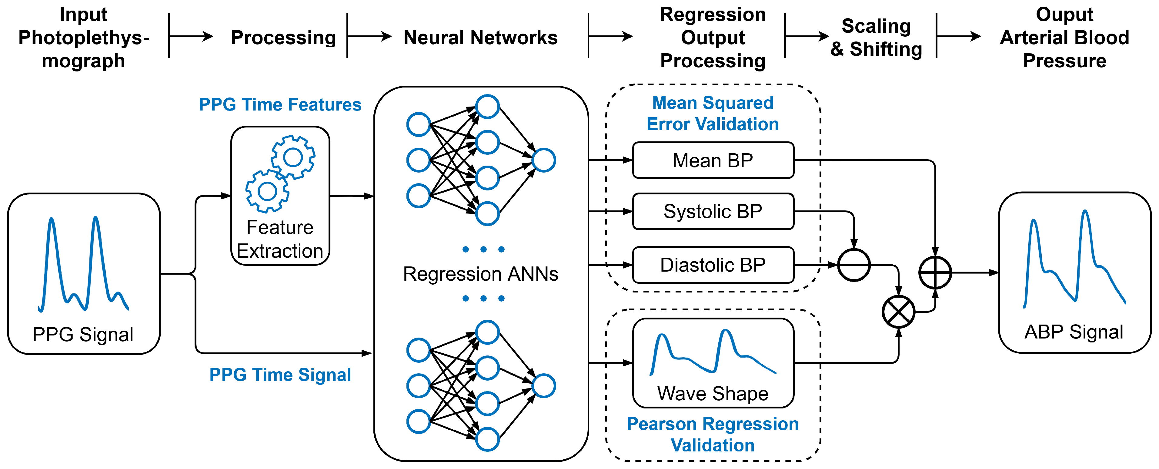
3.3. Machine Learning Approach

The approach to measure the continuous arterial blood pressure waveform using PPG is a two stage process. The waveform shape is the output of one model, but lacks accurate absolute values. In order to correct this, separate models are used to predict the SBP, DBP, and MAP. These discrete values are then used to scale and shift the normalised output waveform to the correct values. This process is summarised in Figure 1.

Using all four models, the ABP wave can be generated using

$$ABP=\left(\frac{AB{P}_0-\overline{AB{P}_0}}{max\left(AB{P}_0\right)-min\left(AB{P}_0\right)}\right)(SBP-DBP)+MAP$$

(3)

where $ABP$ refers to the final ABP waveform and $AB{P}_0$ refers to the output of the waveform neural network. $SBP$, $DBP$, and $MAP$ refer to the denormalised outputs of the discrete blood pressure neural networks.

3.4. Discrete Blood Pressure Prediction

As discussed in Section 1, there are two general approaches to the blood pressure prediction. The first is to use feature extraction and classical machine learning. The second is to use deep learning on an entire segment of the waveform. These two approaches are attempted here, since both show promise in the literature. The aim is to predict the SBP, DBP, and MAP.

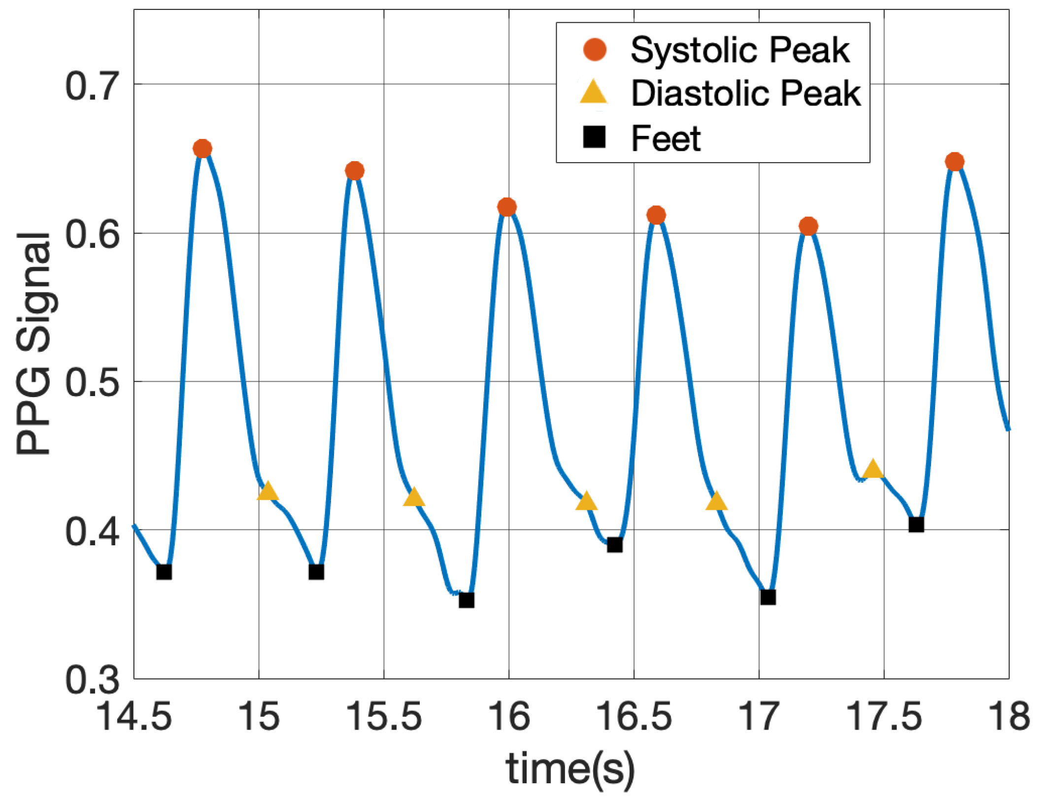
3.4.1. Feature Extraction

Both time domain and frequency domain features were extracted for the classical machine learning approach.

Generalising the feature extraction proved challenging. Elgendi [5] describes features in the PPG wave. As an example, the diastolic point appears as a zero in the PPG’s first derivative [5]. However, in reality, feature extraction is difficult to generalise when the signals are not from young, healthy individuals with ideal waveforms [5]. For example, the dicrotic notch becomes less visible with increased arterial stiffness, such as in Figure 2. Feature extraction was built around reliable identification of the systolic point, diastolic point, and waveform foot. The systolic points correspond to signal peaks, separated by at least 0.24 s (giving a maximum heart rate of 250 bpm). The waveform foot was found by finding the local minimum before a systolic peak. Finally, the diastolic point was identified using a scoring matrix. The matrix considers all the local maxima between the systolic peak and the next foot and takes into account the points’ amplitude, first derivative, and second derivative to find the highest point with the flattest derivative. Extracted systolic points, diastolic points, and feet are shown in Figure 2.

The time domain features are based on those described by Elegendi [5] and Chowdhury et al. [8]. The features considered include:

• Time-related features: systolic upstroke duration, diastolic duration, and duration between systolic peak and diastolic peak.
• Amplitude-features: systolic peak, diastolic peak, foot, augmentation index (ratio of systolic peak-to-diastolic peak).
• Time and amplitude features: systolic width, diastolic width, total width (sum of the systolic and diastolic widths), ratio of systolic to diastolic widths.
• Area features: pulse area (total area under PPG curve over a cardiac cycle), inflection point area (ratio of area post dicrotic notch to area pre-dicrotic notch).
• Frequency-features: respiratory rate, heart rate.

The time and amplitude features and the respiratory rate are worth discussing in more detail.

For the time and amplitude features, a proportion of the total systolic peak amplitude is considered, namely 25, 33, 50, 66, 75, and 90%. The point corresponding to this amplitude is then found during the systolic upstroke and again during diastole. The systolic width is the time from the systolic upstroke point to systolic peak, and the diastolic width is the time from systolic peak to subsequent diastole.

The respiratory rate is found using a frequency analysis. Respiration modulates the blood pressure and introduces a slowly varying sinusoidal component into the PPG signal [24]. Respiratory rates were assumed to have a maximum range between 2.97 breaths per minute and 28.02 breaths per minute [24], or 0.05 Hz to 0.47 Hz. The average respiratory rate was found by taking the Fourier transform of the PPG signal and finding the largest frequency in this band.

3.4.2. Models

A number of machine learning models have been considered. The models considered include artificial neural networks (ANNs) with a regression output, recursive neural networks (RNNs), specifically long short term memory (LSTM) networks, regression support vector machines (SVMs), and convolutional neural networks (CNNs).

There is a difference between the models applied in the deep and classical machine learning approaches. The LSTMs and CNNs are considered for the deep learning approaches only. LSTMs (and RNNs, in general) contain feedback loops within each activation unit, in turn providing the model with memory [11]. This makes them good for sequential data [11]. LSTMs struggle to manage long sequences and, so for, this network only 2 s of PPG data was used for the last 1s of ABP values [11]. CNNs are adept at finding patterns and features within data, and so these were also applied to the sequential waveform data. Regression SVMs, on the other hand, are only applied to the feature dataset since SVMs are generally computationally intensive, and the waveform data is much larger than the feature dataset.

For the ANNs, RNNs, and CNNs, the Adam optimiser was used with a batch size of 128. A mean squared error cost function was used. Datasets were shuffled and split into training, validation, and test sets in a 70-15-15 ratio, respectively. All features and waveforms in each dataset were shifted and scaled to range from −1 to 1. The approach adopted to train the models was to train for 10 epochs, starting with a learning rate of ${10}^{-4}$. From this, the hyperparameters were tuned. If the training loss was decreasing particularly slowly, the learning rate was increased, and if the training loss was fluctuating, then the learning rate was decreased. If the model was underfitting the data (consistently high training and validation losses), then the regularisation parameter was decreased or the model complexity increased. The opposite was performed for an overfit, where there is low training loss and high validation loss. Models were trained until the validation loss did not improve for at least 20 consecutive epochs, with a learning rate of ${10}^{-6}$.

All-in-all, nine machine learning models have been considered, four for the deep learning models and five for the classical learning models. The ANNs considered for both approaches are two layers of 512 activation units and three layers of 512. For the classical approach, an additional four layers of 512 was also implemented. The 1D CNN applied to the full waveform has three convolutional layers. Between each of these are a batch normalisation and rectified linear unit (ReLU) layer. At the output is a global average pooling layer and a regression output [25]. The LSTM follows Paviglianiti et al.’s architecture [11], consisting of three LSTM layers of size 128, separated by a batch normalisation layer. The first LSTM layer in this architecture is bilinear [11]. A regression SVM and a binary decision tree for regression were also applied to the feature dataset.

Results for the discrete blood pressure prediction can be found in Section 4. The machine learning models to predict the waveform shape are discussed in the following section.

3.5. Waveform Prediction

In order to generate the continuous arterial blood pressure waveform, a model is used to output the wave shape.

3.5.1. Processing

Ten seconds of the PPG waveform are used as the input to the network and one second ($t=9$ s $\to t=10$ s) of the ABP waveform is used as the output. With the data’s sampling frequency of $F_s=125$ Hz, this corresponds to 1250 input points and 125 output points. To reduce the number of outputs of the neural network, the output data was down-sampled from 125 Hz to 25 Hz, resulting in 25 output points. The ABP signal has a bandwidth of approximately $F_b=8$ Hz, so the down-sampled frequency of 25 Hz is well above the Nyquist criterion of $F_s\ge 2F_b=16$ Hz. To implement feature scaling, the average mean and average range for both PPG and ABP datasets was calculated. Each signal was then feature scaled as per Equation (4), where $E_s\left[\overline{PPG}\right]$ refers to the expected value (or mean) across the data sample’s means and the denominator refers to the expected value (or mean) of the whole data sample’s ranges. The same computation applies to the ABP signals.

$$PP{G}_{scaled}=\frac{PPG-E_s\left[\overline{PPG}\right]}{E_s[max\left(PPG\right)-min\left(PPG\right)]}$$

(4)

Data observations consisting of the 1250-point PPG signals and the 25-point ABP signals were generated from the data segments, resulting in multiple observations from one segment and a total of over 300,000 observations.

3.5.2. Regression Loss Layer

The neural network to predict the wave shape is required to maximise on the accuracy of the shape. For this, a custom regression layer was created in Matlab, with the loss function altered to use the Pearson correlation coefficient r between the predicted wave shape $A_0$ and the actual wave shape $A_t$, as shown in Equation (5). Since $\left|r\right|\le 1$ and is proportional to correlative strength, taking $1-\left|r\right|$ allows the loss to be minimised, thereby maximising the correlation.

$$\begin{array}{cc}\hfill loss& =1-\left|r\right|\hfill \end{array}$$

(5)

3.5.3. Machine Learning Models

Different models were trained using either the custom Pearson correlation regression loss layer or the standard mean absolute error loss. The final model will first be discussed, after which a brief description of the other models will be provided.

The final network is a sequence-to-sequence regression network consisting of the input layer, three hidden layers, and the output layer, which used the custom Pearson correlation loss function. The hidden layers are standard fully connected (fc) layers of 1024 neurons each, followed by batch normalisation layers and rectified linear unit (ReLU) activation layers. It is common to use ReLU activation, since they are computationally inexpensive and prevent vanishing gradients. Activation layers were followed by dropout layers with dropout factors of 0.2. The dropout factors result in a proportion of neurons being ignored, which prevents over fitting [26]. It effectively simulates many more architectures with different numbers of units in the layers. The architecture is illustrated in Figure 3.

A total of 70% of the observations were used to train the model, with 15% used for validation during training and the remaining 15% for testing. The model was trained using the stochastic gradient descent with momentum (SGDM) optimiser.

Other architectures were attempted, but only those which achieved over 0.75 correlation (as seen in Section 4) are discussed. Since the objective is to output a time-series waveform, various architectures involving LSTM networks and bidirectional LSTM (biLSTM) networks were modeled. The second approach used standard ANN fully connected layers in different configurations, which only produced correlated results when used with a Pearson correlation regression loss layer. A summary of the different architectures is presented in

Table 1. Results of various neural network architectures for waveform regression. Row 1 corresponds to the final model chosen.

#	Description
1	3 fully connected 1024 layers with batch normalisation, ReLU, and 0.2 dropout, using Pearson correlation regression layer
2	2 layers with 1024 bilstm units, with 0.2 dropout factors, with a standard regression layer
3	2 layers with 1024 bilstm units, with 0.2 dropout factors solved using the Adam optimiser, with a standard regression layer
4	2 layers with 1024 bilstm units, with 0.2 dropout factors, using the Pearson correlation regression layer
5	2 layers with 1024 lstm units, with 0.2 dropout factors, using a standard regression layer
6	2 layers with 1024 lstm units, with 0.2 dropout factors, using the Pearson correlation regression layer

.

3.6. Testing

All the machine learning models are supervised. Thus, we compare the network prediction with the known ground truth values. As previously mentioned, the dataset was split into 70% for training, 15% for validation (during training), and 15% for testing. For the SBP, DBP, and MAP, the ground truth values are the pressures extracted from the ABP waveform, while for the waveform prediction, we compare with the ABP signal itself. The metrics used for the networks differ. For the discrete blood pressure prediction, the mean average error and coefficient of determination are calculated. Additionally, the percentage of predictions with an error less than 10 mmHg is specified. For the waveform prediction, the Pearson r value is compared between architectures. A further description of these metrics is found in Section 4.

4. Results

For the discrete blood pressure prediction, all nine machine learning models were trained and then evaluated on the testing dataset. Results from training the machine learning models are shown in

Table 2. SBP, DBP, and MAP Results from Trained Machine Learning Models.

Model		SBP			DBP			MAP
		MAE	% Error	${\mathit{R}}^2$	MAE	% Error	${\mathit{R}}^2$	MAE	% Error	${\mathit{R}}^2$
			<10 mmHg			<10 mmHg			<10 mmHg
	ANN (2 × 512)	14.0	46.5	0.110	6.62	79.4	0.158	7.34	72.9	0.250
Full	ANN (3 × 512)	13.8	47.3	0.148	6.54	80.0	0.158	7.16	74.3	0.274
Waveform	LSTM	22.5	27.1	−0.819	22.2	10.1	−0.0513	9.24	60.3	−0.0754
	CNN	16.1	35.8	0.00	21.6	10.7	0.00	8.79	62.4	0.00
	ANN (2 × 512)	5.73	83.7	0.777	2.96	95.8	0.692	3.27	94.5	0.771
Feature	ANN (3 × 512)	5.32	86.5	0.780	3.50	94.9	0.614	3.65	94.2	0.750
Extraction	ANN (4 × 512)	5.26	86.1	0.798	3.39	94.9	0.629	3.30	94.1	0.745
	Binary Tree	7.46	77.0	0.485	3.58	90.2	0.404	4.27	86.7	0.477
	Reg. SVM	13.8	44.4	−0.769	6.11	84.5	0.0779	7.13	74.9	0.186

. Each algorithm was evaluated on the MAE for the unseen test data, the acceptable proportion (percentage of predictions with an error less than 10 mmHg, as per the standard discussed in Section 2), and the coefficient of determination ($R^2$). Based off of the standard for blood pressure prediction, the passing population should be at least 85% for the model to be considered adequate. The $R^2$ value indicates how well-correlated the predicted blood pressure is with the actual blood pressure [27]. It is used because a large proportion of the blood pressures fall within a relatively narrow range. A model that outputs the mean blood pressure may appear to do well, based off of the MAE and passing population, but is of no use. Such a model would have an $R^2$ close to 0, indicating that the two variables are independent and uncorrelated [27]. $R^2$ is not calculated by squaring another parameter and can yield a negative result in circumstances when the best-fit line exhibits a worse fit than a horizontal line [27]. Results are further discussed in Section 5.

From the three models that performed best on SBP, DBP, and MAP, respectively, a scatter plot is presented in Figure 4. This shows the predicted blood pressure against the actual blood pressure.

The main performance metric used for the waveform network is Pearson’s r value, with a higher value corresponding to higher correlation. The final model, consisting of three hidden layers of 1024 neurons and a Pearson correlation regression layer, achieved a strong r value of 0.864 across the testing data. This result, as well as the results from the other models discussed in Section 3.5.2, are shown in

Table 3. Results of various neural network architectures for waveform regression. Row 1 corresponds to the final model chosen.

#	Structure	Regression	r
1	3 × fc(1024)	Pearson	0.864
2	2 × bilstm(1024)	Standard	0.801
3	2 × bilstm(1024) 1	Standard	0.797
4	2 × bilstm(1024)	Pearson	0.802
5	2 × lstm(1024)	Standard	0.781
6	2 × lstm(1024)	Pearson	0.818

¹ Using Adam optimising algorithm.

.

Complete ABP data was generated as per the algorithm in Section 3.3. An example of a normotensive sample and a hypertensive sample is shown in Figure 5a,b, respectively.

5. Discussion

In the discrete blood pressure models, the feature extraction models consistently outperform the deep learning models. For SBP, only the two larger feature-trained ANNs meet the 85% criterion. For DBP and MAP, all feature-trained ANNs and the binary decision tree meet the criterion. None of the deep learning models trained on the full waveform meet the criterion, although the ANNs for the DBP do come relatively close.

It is worth examining the deep learning models’ performance. The LSTM and CNN models have very low $R^2$ values, and the CNN actually produces a constant value for the DBP and MAP. This shows these models are underfitting the data. The results produced by the ANNs on the full wave are similar to those achieved by Slapničar et al. [14], who, at best, achieved an MAE of 9.42 mmHg and 6.88 mmHg for SBP and DBP, respectively. No other performance metrics are given in the paper. Paviglianiti [11] achieved far lower MAEs; however, the study only includes 121 patients. In fairness, those discrete valued predictions made use of a ResNet-18 architecture. This was not implemented because it is not described how the 1D signal data was resized for the ResNet architecture (which is intended for 2D images of size 224 by 224) or whether the tens of layers in ResNet-18 were all rewritten for 1D signals. This being said, none of the four other deep learning approaches in this study achieved acceptable results, and the Paviglianiti et al.’s models still had relatively low $R^2$ values (approximately 0.3 to 0.4). Athaya and Choi [12] also achieved effective results with deep learning (low MAE and high $R^2$), using only 100 subjects. In both papers, it is possible that the models would not generalise well for larger sample sizes, though this remains to be tested. This does not mean that the deep learning approach is not of value. It greatly simplifies the signal processing by cutting out the feature extraction. It is possible that with more complex architectures (such as ResNet [11], or U-Net [12]) and/or more hyperparameter tuning the deep learning approach will yield better results.

For the best performing models (the two-layered feature ANNs for DBP and MAP and the four-layered feature ANN for SBP), the standard deviation (SD) of error has also been calculated. The SBP’s test error (MAE ± SD) is 5.26 ± 6.53 mmHg. For DBP it is 2.96 ± 3.31 mmHg and for MAP the test error is 3.27 ± 3.55 mmHg. All meet the minimum criterion in [15].

Both LSTM and fully connected ANN networks show potential for the estimation of the wave shape, especially when modified to maximise on this shape specifically and not the absolute values. However, the simpler ANN network is both more computationally efficient and yields a higher correlation. The average waveform Pearson correlation of 0.864 implies that the waveform output is strongly correlated to the reference waveforms. In the literature survey, the maximum Pearson’s correlation was achieved by Athaya and Choi [12], using a U-net architecture that yielded a correlation of 0.993. However, there are two key differences. Firstly, the study by Athaya and Choi used only 100 subjects, whereas this study used data from 1669 patients. Secondly, the PPG and ABP signals were phase-matched before training the models. Using phase matching before implementing the architectures outlined in this study may yield better results with a far more computationally efficient model, compared to the study by Athaya and Choi.

The successful feature extraction models confirm part of the study’s main aim. The focus is on whether it is possible for PPG to provide a clinically viable, low-cost, cuffless, non-invasive, and continuous blood pressure measurement system. PPG inherently provides a cuffless, non-invasive, and continuous signal. The successful models also strongly suggest the use of PPG provides measurements that are clinically viable from an accuracy perspective.

5.1. Significance of Results

Given that pulse oximeters are ubiquitous in hospitals and healthcare environments, with portable oximeters rising in popularity during the COVID-19 pandemic, it would be easy to deploy this approach within the established systems. This makes the model an attractive solution to continuous blood pressure measurement, especially in the context of low and middle income countries (LMICs), where healthcare settings are often resource-constrained. Blood pressure determination, in this way, would allow for a combined pulse oximetry and blood pressure measurement system, leading to increased patient comfort and faster care, thus freeing up healthcare workers. Adapting the system to operate on wearable health devices could also allow comfortable at-home monitoring of hypertensive patients.

5.2. Recommendations for Further Work

In order to make the model more accurate, access to the MIMIC-III clinical records should be sought. This will allow accuracy across demographics to be determined and an inclusive dataset to prevent biases to be constructed. Owing to the lack of clinical data, it is not known how well the model performs based on an individual’s age or sex. Additionally, the bias in the dataset means there is a lack of waveforms from individuals outside an ICU setting (including healthy individuals and outpatients). The model should be tested on such populations, as well as those with a variety of known conditions (such as atrial fibrillation), as described in [15].

Limitations of PPG and the effect of skin tone, patient motion, and perfusion should also be investigated. This fits well with exploring hardware implementations of the model. The waveform prediction may also be improved using techniques such as compressive sensing or non-linear approximation. Despite these limitations, the results are promising and could be a step towards changing one of the most fundamental clinical measurements.

6. Conclusions

This study presents the use of PPG to achieve continuous non-invasive blood pressure measurement. The MIMIC-III waveform database base was used and its data processed, ultimately yielding a sample size of 1669 patients comprising 890 h of data. Models were developed using machine learning to determine discrete blood pressure values (SBP, DBP, and MAP), as well as the waveform shape. For the discrete BP prediction, three regression ANNs were the most successful, and the SBP, DBP, and MAP models have errors of 5.26 ± 6.53 mmHg, 2.96 ± 3.31 mmHg, and 3.27 ± 3.55 mmHg, respectively. In all three models, over 85% of predictions have an error less than 10 mmHg, meeting the AAMI/ESH/ISO standard. For waveform prediction, a regression ANN with a custom loss layer yielded a strong correlation of 0.864.

This study demonstrates a non-invasive blood pressure measurement technique that could improve patient management in a variety of clinical scenarios. Further investigations into the models’ performance in different populations is required, and improvements may be achieved by training on a wider population outside of MIMIC-III’s ICU patients.

References

1. Rehman, S.; Nelson, V.L. Blood Pressure Measurement, 2021. Available online: https://www.ncbi.nlm.nih.gov/books/NBK482189/ (accessed on 19 October 2021).
2. Pittman, J.A.L.; Ping, J.S.; Mark, J.B. Arterial and central venous pressure monitoring. Int. Anesthesiol. Clin. 2004, 42, 13–30. [Google Scholar] [CrossRef] [PubMed]
3. Denardo, S.J.; Nandyala, R.; Freeman, G.L.; Pierce, G.L.; Nichols, W.W. Pulse Wave Analysis of the Aortic Pressure Waveform in Severe Left Ventricular Systolic Dysfunction. Circ. Heart Fail. 2009, 3, 149–156. [Google Scholar] [CrossRef] [PubMed] [Green Version]
4. Hager, H.H.; Burns, B. Artery Cannulation, 2021. Available online: https://www.ncbi.nlm.nih.gov/books/NBK482242/ (accessed on 19 October 2021).
5. Elgendi, M. On the Analysis of Fingertip Photoplethysmogram Signals. Curr. Cardiol. Rev. 2012, 8, 14–25. [Google Scholar] [CrossRef] [PubMed]
6. Wang, R.; Jia, W.; Mao, Z.H.; Sclabassi, R.J.; Sun, M. Cuff-free blood pressure estimation using pulse transit time and heart rate. In Proceedings of the 2014 12th International Conference on Signal Processing (ICSP), Hangzhou, China, 19–23 October 2014; pp. 115–118. [Google Scholar] [CrossRef] [Green Version]
7. Kurylyak, Y.; Lamonaca, F.; Grimaldi, D. A Neural Network-based method for continuous blood pressure estimation from a PPG signal. In Proceedings of the 2013 IEEE International Instrumentation and Measurement Technology Conference (I2MTC), Minneapolis, MN, USA, 6–9 May 2013; pp. 280–283. [Google Scholar] [CrossRef]
8. Chowdhury, M.H.; Shuzan, M.N.I.; Chowdhury, M.E.; Mahbub, Z.B.; Uddin, M.M.; Khandakar, A.; Reaz, M.B.I. Estimating Blood Pressure from the Photoplethysmogram Signal and Demographic Features Using Machine Learning Techniques. Sensors 2020, 20, 3127. [Google Scholar] [CrossRef] [PubMed]
9. Teng, X.; Zhang, Y. Continuous and noninvasive estimation of arterial blood pressure using a photoplethysmographic approach. In Proceedings of the 25th Annual International Conference of the IEEE Engineering in Medicine and Biology Society (IEEE Cat. No.03CH37439), Cancun, Mexico, 17–21 September 2003; Volume 4, pp. 3153–3156. [Google Scholar] [CrossRef]
10. Yoon, Y.Z.; Yoon, G.W. Nonconstrained Blood Pressure Measurement by Photoplethysmography. J. Opt. Soc. Korea 2006, 10, 91–95. [Google Scholar] [CrossRef] [Green Version]
11. Paviglianiti, A.; Randazzo, V.; Villata, S.; Cirrincione, G.; Pasero, E. A Comparison of Deep Learning Techniques for Arterial Blood Pressure Prediction. Cogn. Comput. 2021, 14, 1689–1710. [Google Scholar] [CrossRef] [PubMed]
12. Athaya, T.; Choi, S. An Estimation Method of Continuous Non-Invasive Arterial Blood Pressure Waveform Using Photoplethysmography: A U-Net Architecture-Based Approach. Sensors 2021, 21, 1867. [Google Scholar] [CrossRef] [PubMed]
13. El-Hajj, C.; Kyriacou, P.A. A review of machine learning techniques in photoplethysmography for the non-invasive cuff-less measurement of blood pressure. Biomed. Signal Process. Control 2020, 58, 101870. [Google Scholar] [CrossRef]
14. Slapničar, G.; Mlakar, N.; Luštrek, M. Blood Pressure Estimation from Photoplethysmogram Using a Spectro-Temporal Deep Neural Network. Sensors 2019, 19, 3420. [Google Scholar] [CrossRef] [PubMed] [Green Version]
15. Stergiou, G.S.; Alpert, B.; Mieke, S.; Asmar, R.; Atkins, N.; Eckert, S.; Frick, G.; Friedman, B.; Graßl, T.; Ichikawa, T.; et al. A Universal Standard for the Validation of Blood Pressure Measuring Devices: Association for the Advancement of Medical Instrumentation/European Society of Hypertension/International Organization for Standardization (AAMI/ESH/ISO) Collaboration Statement. Hypertension 2018, 71, 368–374. [Google Scholar] [CrossRef] [PubMed]
16. Moody, B.; Moody, G.; Villarroel, M.; Clifford, G.; Silva, I. MIMIC-III Waveform Database (version 1.0). PhysioNet 2020, 3. [Google Scholar] [CrossRef]
17. Johnson, A.; Pollard, T.; Shen, L.; Lehman, L.; Feng, M.; Ghassemi, M.; Moody, B.; Szolovits, P.; Celi, L.; Mark, R. MIMIC-III, a freely accessible critical care database. Sci. Data 2016, 3, 160035. [Google Scholar] [CrossRef] [PubMed] [Green Version]
18. Goldberger, A.; Amaral, L.; Glass, L.; Hausdorff, J.; Ivanov, P.; Mark, R.; Stanley, H. PhysioBank, PhysioToolkit, and PhysioNet: Components of a new research resource for complex physiologic signals. Circulation 2000, 101, 215–220. [Google Scholar] [CrossRef] [PubMed] [Green Version]
19. PhysioNet. Open Data Commons Open Database License v1.0. Available online: https://physionet.org/content/mimic3wdb/view-license/1.0/ (accessed on 21 February 2023).
20. Johnson, A.; Pollard, T.; Mark, R. MIMIC-III Clinical Database (version 1.4). PhysioNet 2016. [Google Scholar] [CrossRef]
21. PhysioNet. The WFDB Software Package. Available online: https://archive.physionet.org/physiotools/wfdb.shtml#intro (accessed on 25 October 2012).
22. Harfiya, L.N.; Chang, C.C.; Li, Y.H. Continuous Blood Pressure Estimation Using Exclusively Photopletysmography by LSTM-Based Signal-to-Signal Translation. Sensors 2021, 21, 2952. [Google Scholar] [CrossRef] [PubMed]
23. Freedman, D.; Pisani, R.; Purves, R. Statistics (International Student Edition), 4th ed.; WW Norton & Company: New York, NY, USA, 2007. [Google Scholar]
24. Addison, P.S.; Watson, J.N.; Mestek, M.L.; Mecca, R.S. Developing an algorithm for pulse oximetry derived respiratory rate (RRoxi): A healthy volunteer study. J. Clin. Monit. Comput. 2012, 26, 45–51. [Google Scholar] [CrossRef] [PubMed] [Green Version]
25. Wang, Z.; Yan, W.; Oates, T. Time Series Classification from Scratch with Deep Neural Networks: A Strong Baseline. In Proceedings of the 2017 International Joint Conference on Neural Networks (IJCNN), Anchorage, AK, USA, 14–19 May 2017; pp. 1578–1585. [Google Scholar]
26. Srivastava, N.; Hinton, G.; Krizhevsky, A.; Sutskever, I.; Salakhutdinov, R. Dropout: A Simple Way to Prevent Neural Networks from Overfitting. J. Mach. Learn. Res. 2014, 15, 1929–1958. [Google Scholar]
27. Chicco, D.; Warrens, M.J.; Jurman, G. The coefficient of determination R-squared is more informative than SMAPE, MAE, MAPE, MSE and RMSE in regression analysis evaluation. PeerJ Comput. Sci. 2021, 7, e623. [Google Scholar] [CrossRef] [PubMed]
Figure 1. A block diagram depicting the overall system of determining the ABP waveform from the PPG signal.
Applsci 13 03955 g001
Figure 2. PPG waveform displaying poorly visible dicrotic notch and diastolic point. The extracted systolic points, diastolic points, and waveform feet are shown as circles, triangles, and squares, respectively.
Applsci 13 03955 g002
Figure 3. Waveform neural network architecture. FC refers to a fully connected layer.
Applsci 13 03955 g003
Figure 4. Scatter plot of predicted blood pressure against actual blood pressure for SBP, DBP, and MAP. The models used for the prediction are those that gave the best performance, specifically the 2-layered feature-trained ANN for DBP and MAP and the 4-layered feature-trained ANN for SBP.
Applsci 13 03955 g004
Figure 5. Generated ABP Waveforms using neural network models.
Applsci 13 03955 g005