A Numerical Investigation of Transformation Rates from Debris Flows to Turbidity Currents under Shearing Mechanisms

Abstract

The evolution of a submarine landslide is a very complicated process due to slurry–water interactions. Most previous studies have focused on debris flows or turbidity currents independently. Little research has been conducted on the processes of transformation from debris flows into turbidity currents. Moreover, the underlying mechanical mechanisms of these transformation processes are not well understood. In this study, we aimed to better understand these mechanisms by simulating submarine landslide transportation processes using computational fluid dynamics. In the numerical models, the two-phase mixture module was adopted to mimic the interactions of the slurry with the ambient water, which we validated through a dam-break case. Here, the rheological behaviors of the slurries are described using the Herschel–Bulkley model. A formula for transformation rates is best fitted through a case series of debris flows. In particular, the activation stress is expressed by the dynamic pressure at the moment when the slurry starts to mobilize, which is fitted as a coefficient 6.55 × 10⁻⁵ times the shear strength. Then, two coefficients in the formula of the transformation rate are fitted as 1.61 and 0.26, respectively, based on the cases of debris flows, considering their different initial thicknesses, levels of slurry consistency and slope angles. Finally, in a real-scale debris flow case study, we demonstrate that the slurry is fully transformed before it is deposited. The expected outcome, the mechanical theory, the activation stress and the transformation rate would be applied to assess the influence area of the realistic turbidity currents and their harm to the subsea environment.

1. Introduction

Submarine landslides are one of the most significant submarine geo-hazards [1]. The sliding masses may cause seabed mobilizations and foundation failures, thus undermining the safety of offshore engineering structures and affecting the exploitation of offshore energy resources [2,3,4]. Submarine landslides generally have the characteristics of large volumes, quick sliding velocities and lengthy migration durations [5], and they may occur on slopes with small angles [6]. The factors triggering submarine landslides include earthquakes, rapid sedimentation, hydrate dissociation, salt diapirism and weathering [7].

Debris flows, the product of the submarine landslide (Figure 1) [8], are dense, and viscous sediment–water mixtures that move downslope as an agglomeration are characterized as gravity flows with non-Newtonian rheological properties, typically in a laminar state [9]. Turbidity currents are diluted currents that have high concentrations of suspended materials. The majority of previous studies have mainly concentrated on debris flows or turbidity currents independently, regardless of the important transformation processes that occur between them [10]. Mohrig et al. [11] demonstrated that the front of the debris flow can hydroplane on water layers with small thickness values. The effects Aof the onset mechanism and initial slope during the flow evolution and related changes in the bed morphology were investigated by Huang et al. [12]. Liu et al. [13] studied the impacts of clay/sand compositions on the depositional mechanism of debris flows through physical experiments and numerical simulations. Wells and Dorrell [14] investigated the turbulence processes within turbidity currents using experimental tests and numerical simulations.

However, the processes of transformation from debris flows into turbidity currents have seldom been studied. Moreover, the mechanical mechanisms of these transformation processes are not clear. It should be noted that a good understanding of these mechanical mechanisms requires one to thoroughly consider the complicated dilution activities between the sediment grains and the ambient water [15]. Another perplexing problem regarding debris flows is why some remain compact during transportation while others significantly dissolve and transform into two separate flows [16]. Related to these puzzles, some quantitative parameters need to be derived ahead, such as the activation threshold stress of the transformation and the transformation rate. The reason for the ignorance of these important processes is the difficulties to investigate them. Various parameters, including velocity, density, impact pressure and sliding distance, significantly change during the transformation from debris flows into turbidity currents due to their characteristic differences [17]. There is still a lack of real in situ observational data that can be used to investigate these transformation mechanisms due to the harsh underwater environments. Flume experiments have been performed with small volumes of artificial slurries sliding along a channel [18]. To ensure the flowability, the sliding materials in the experiments typically have high water contents and low strengths (e.g., ~0.1 kPa), and the strength is approximately two orders of magnitude lower than that of a genuine slide in its undamaged state.

Numerical modeling may be helpful to investigate the transformation mechanism from the debris flow to the turbidity current. Small-scale events observed in the lab can be simulated using numerical models, which can subsequently be extended to the field scale [19]. This may be a more effective way to investigate the transformation mechanisms. In this paper, the computational fluid dynamics (CFD) method is adopted to investigate the mechanisms of transformation from debris flows into turbidity currents. Moreover, we use the Herschel–Bulkley (H-B) model [20] to describe the rheological behaviors of slurries. Emphasis is placed on the shearing and mixture behaviors on the upper surface of the debris flow, which is characterized by the velocity gradient at the interface and the diluted flows, respectively. The effects of key factors on the transformation are examined, and the transformation efficiency is quantified using a metric called the transformation rate. Then, a case study of a real-scale debris flow is conducted to estimate the transformation volume.

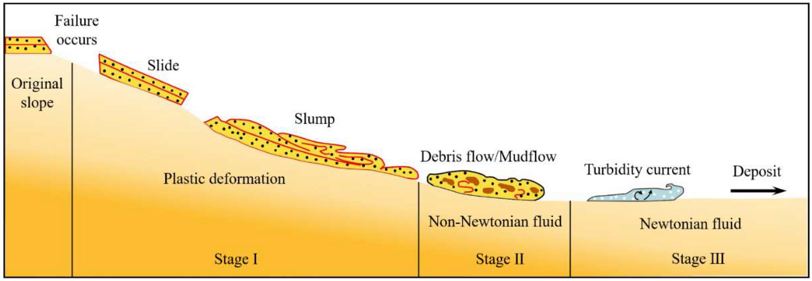
2. Transformation Mechanisms

As qualitatively described by Felix and Peakall [21], there are six different mechanisms of transformation from debris flows into turbidity currents: liquefaction; breaking up of the flow; shearing on the top, leading to erosion; mixing due to instability and wave formation; mixing under and into the flow head; and hydraulic jump. However, an accurate assessment of the contribution of each individual mechanism to the transformation process remains to be performed, and a better understanding of the mechanical theory behind the transformation phenomenon is still needed [22]. Herein, for the sake comprehensiveness, the six transformation mechanisms are briefly discussed.

2.1. Liquefaction

When the pore water pressure exceeds the inter-grain cohesions, the stresses in the grain skeleton decrease to nil, and then the fine grains can be liquefied [23]. When a debris flow with fine grains is partly or entirely liquefied, a turbidity current is generated, with the pore water being fully mixed with the ambient water. Since clays are often characterized by high cohesion between particles, debris flows carrying clay particles are difficult to liquefy [24,25].

2.2. Breaking Up of Flow

Debris flows are originally composed of materials with well-developed internal structures [26]. The disturbance accompanying the movement of the material gradually destroys the original structures and causes the collapse of the sliding body. This tends to result in the disintegration of the sliding mass within the debris flow. Therefore, the ambient water will be mixed with the sliding mass with collapsed internal structures and appear to be transformed into a turbidity current.

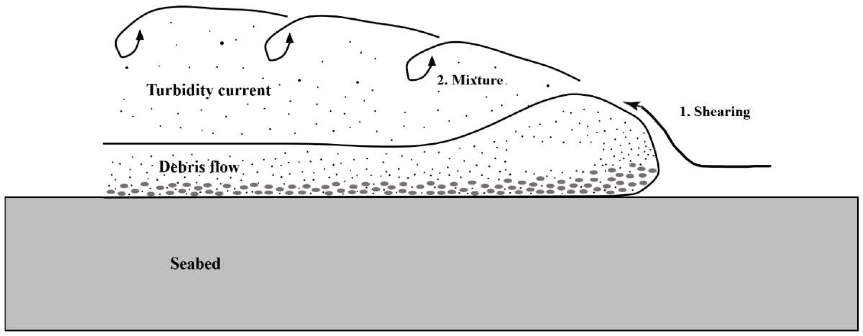
2.3. Shearing on Top Leading to Erosion

Given a sufficiently high flow velocity and a relatively low underflow viscosity, shearing frequently occurs on the upper surface of a debris flow [27]. The original flow then separates into two layers, namely, the turbidity current on the upper surface and the debris flow at the bottom. The turbidity current moves as an independent part, possibly over a longer distance than the debris flow [22]. This kind of dilution is mainly attributed to the erosion of materials from the crest of the flow to the tail. This indicates that the original debris flow’s shear consistency is a key factor in determining the transformation efficiency. Thus, the well-established erosion theory can be applied to study turbidity currents [18].

2.4. Mixing due to Instability and Wave Formation

For debris flows with loose grains, the ambient water mixes with the sliding material and causes the front of the flow to collapse under its impact. This fluid transformation occurs mostly under conditions where sandy debris flows have high-pore water pressures and when a longer time is required for adequate mixing to occur [28].

2.5. Mixing under and into the Head of the Flow

Based on the relative locations with a stagnation point, the water body may be separated into two upper and lower parts. The upper part will form a cycle in the heads of the fluid and the mixing fluid so that the fluid’s dilution will cause the formation of turbidity currents [29].

2.6. Hydraulic Jump

A hydraulic jump can cause the dilution of the debris flow [30]. When a sandy debris flow rapidly flows into a less dense fluid with a lower velocity, a hydraulic jump occurs. The lower sandy debris flow ceases to move while the top fluid continues to move. Thus, fluid transformation occurs [31]. However, this fluid transformation mechanism can only account for a small part of the high-density fluid transformation.

It should be noted that the above six transformation mechanisms are not always independent [32]. They may be co-existent and can be factors that trigger one another [33]. For example, water and soil mixing at the head and shearing on the top of the flow, causing erosion, often occur together. Therefore, the accurate evaluation of the contributions of these six mechanisms to the whole transformation process is still challenging [22]. The mechanisms can be affected by the original material compositions, such as the concentration, cohesion and sand percentage. This paper focuses on the shearing mechanism acting on the debris flow head and the mixture mechanism acting on the top of the flow (Figure 2).

3. Methodology

3.1. Numerical Models

Various computational techniques have been employed to simulate the evolutions of turbidity currents and undersea debris flows. These techniques include one- and two-dimensional shallow water equations [34], the finite element method [35], the finite volume method [36], the smoothed particle hydrodynamics (SPH) method [37], the finite difference method [38], the material point method [39], the CFD method and the arbitrary Lagrangian–Eulerian method [40,41]. Compared with the other methods (e.g., SPH and MPM), the CFD describes a fluid by describing the density and energy of the material passing through the coordinate points, which is more in line with the characteristics of the water–soil energy exchange during the sliding process. Therefore, in this study, the CFD method, together with the multiphase flow theory, is used to simulate the transformation process using a commercial package, ANSYS fluent.

In previous studies using the CFD, debris flows, treated as bed loads, were frequently simulated using a multi-phase model of the volume of fluid (VOF) or the mixture, while turbidity currents, considered as suspended loads, were modelled using single-phase fluids with specific solid concentrations. Note that the VOF model uses a technique for tracking interfaces on a Eulerian mesh [42], being used for interactions between two or more fluids when the locations of the interfaces between two fluids are crucial. Due to this explicit link, the VOF model can effectively capture the impact of shearing during the transformation from debris flows into turbidity currents [43]. In addition, the volume fraction and turbulence formation can be used to represent the outcome of the turbidity current. However, the mixture between the diluted debris flow and the ambient water cannot be represented. In comparison, the interacting phases can undergo interpenetration in the mixture model [44]. As a result, the mixture model can be used to characterize the mixing process of turbidity currents after the impact of shearing between the debris front and the ambient water is analyzed. Herein, the mixture model is chosen for the later analyses.

3.2. Two-Phase Flow Module

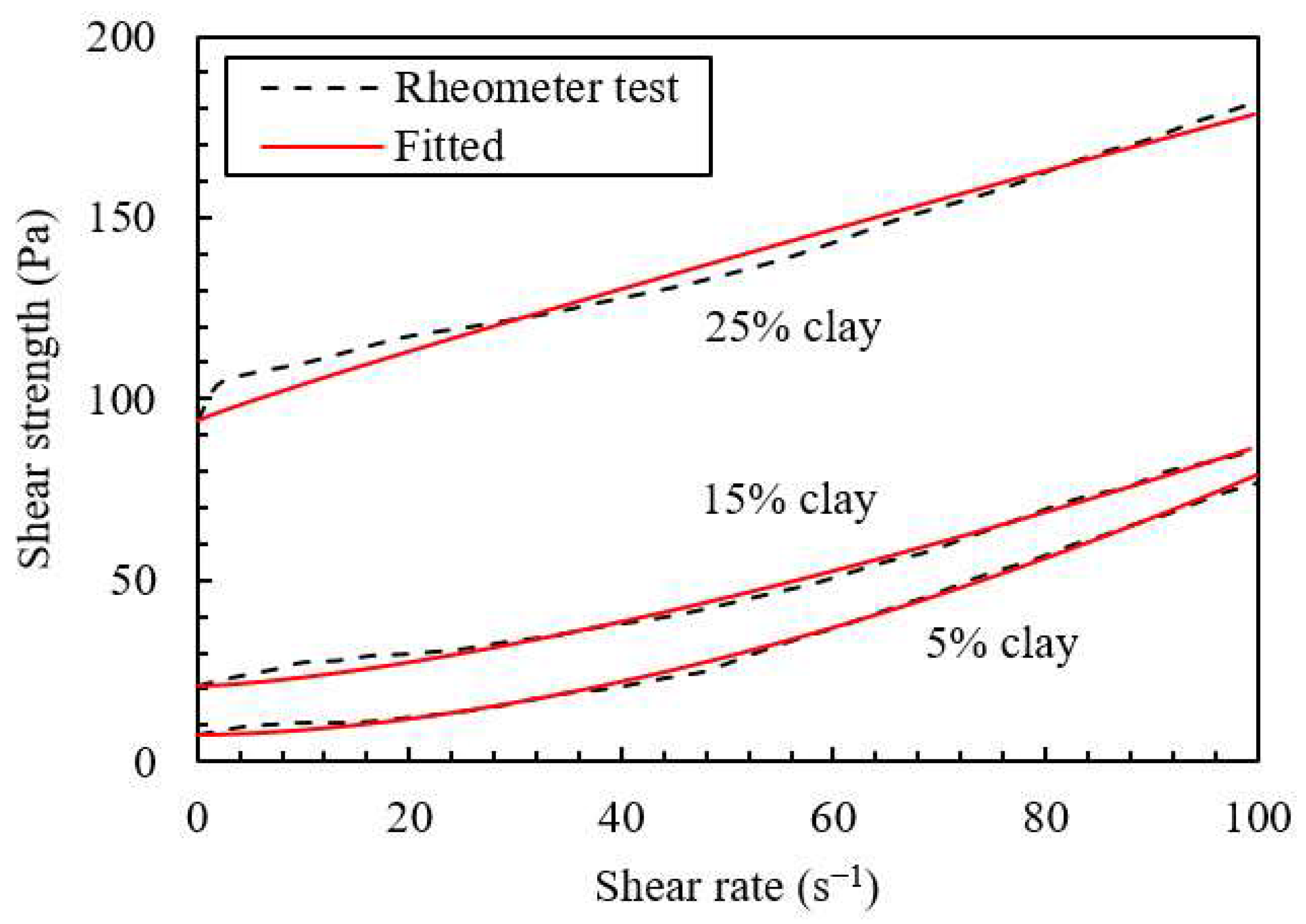
Debris flows and turbidity currents are modelled using two-dimensional Navier–Stokes equations [45]. The surrounding water and the flow material are treated as two distinct fluids, and their properties are computed using the pressure, volume fraction, density and velocity fields. In this study, the submerged sediments are viewed as a monophasic isotropic continuum, and it is believed that both the water and sediments are incompressible. Consequently, the interstitial fluid’s mobility is disregarded, the slope is considered to be impermeable and rigid and the erosion of the seabed induced by the flow is disregarded.

The mass continuity for the flow is described as follows:

$$\frac{\partial \rho }{\partial t}+\nabla \cdot \left(\rho V\right)=0$$

(1)

where ρ denotes the density of the flow, t represents the elapse time and V represents the volume of the flow. When the mixture variables are considered, the momentum equation can be expressed as follows:

$${\rho }_m\left[{\left(V_m\right)}_{,t}+\left(V_m\cdot \nabla \right)V_m\right]=-\nabla P_m+{\rho }_{m}g+\nabla \cdot \left[{\mu }_m\left(\nabla V_m+\nabla V_m{}^T\right)\right]+F_m+\nabla \cdot \left({\displaystyle \sum _{k=1}^n{\alpha }_k{\rho }_k}{V}_k^r{V}_k^r\right)$$

(2)

where ${\rho }_m$, ${\mu }_m$ and $V_m$ are the mixture properties, which are defined as follows:

$${\rho }_m={\displaystyle \sum _{k=1}^n{\alpha }_k}{\rho }_k$$

(3)

$${\mu }_m={\displaystyle \sum _{k=1}^n{\alpha }_k}{\mu }_k$$

(4)

$$V_m=\frac{1}{{\rho }_m}{\displaystyle \sum _{k=1}^n{\alpha }_k}{\rho }_k{V}_m$$

(5)

$\nabla P_{\mathrm{m}}$ denotes the pressure of the mixture and is defined by the following:

$$\nabla P_m={\displaystyle \sum _{k=1}^n{\alpha }_k}\nabla P_k$$

(6)

The phase pressures are generally assumed to be equal at the interface, i.e., P_k = P_m. F_m is a term that depends on the geometry of the interface and accounts for the effect of the surface tension force on the mixture. It is defined as follows:

$$F_m={\displaystyle \sum _{k=1}^n{F}_k}$$

(7)

The diffusion stress phrase, $\nabla \cdot \left({\displaystyle \sum _{k=1}^n{\alpha }_k{\rho }_k}{V}_k^r{V}_k^r\right)$, is used to describe the momentum diffusion induced by relative motions.

Various rheology models including the Bingham model [46], the power law model [47] and the Herschel–Bulkley model [48] have been applied to model the flow characteristics of debris flows and turbidity currents. Among these models, the Herschel–Bulkley model, which offers a more precise representation of the fluid transformation processes and the rheological properties [48,49], is used in this research.

3.3. Validation

Here, to verify the reliability of the multi-phase framework, a dam break experiment is numerically reproduced. In the original laboratory study, the slurry was instantly poured into a rectangular flume from an upstream reservoir, and the front positions of the flow were monitored in real time [50]. A two-dimensional (2D) numerical simulation was used in the computational domain of 12 m × 0.5 m, with the initial configuration shown in Figure 3a. For meshing, quadrilateral elements were used to discretize the entire domain. A convergence study was conducted to determine the desired mesh, and it was found that meshing with a grid cell size of 10 mm × 10 mm is sufficient to achieve accurate results. The mixture model and the laminar model were used as the multi-phase flow model and the viscosity model, respectively. To solve the multi-phase model, a pressure-based solver with an algorithm considering the coupling of pressure and velocity and the SIMPLEC algorithm were used. A second-order implicit scheme and a second-order upwind scheme were also adopted to discretize the momentum formula and the time integration, respectively. Here, the slurry density is ρ_s = 1073 kg/m³. No slip is assumed to occur along the interfaces between the base and the slurry wall. As a function of the shear strain rate, the shear stress in the run-out can be roughly predicted using the following equation [51]:

$$s_{\mathrm{u},\mathrm{B}}=s_{\mathrm{u}0,\mathrm{B}}+\eta \dot{\gamma }$$

(8)

where s_u,B is the mobilized shear stress, s_u0,B denotes the yield stress under static loading and is selected as 42.5 Pa, η represents the plastic viscosity taking a value of 0.0052 Pa·s, and γ represents the shear strain rate. The following formula is adopted to estimate the time step $\mathsf{\Delta }t$ used in the simulations (ANSYS, 2011):

$$\Delta t=\frac{\beta d_{\min }}{v}$$

(9)

where β denotes a coefficient taking a value of 0.4, d_min denotes the minimum mesh size and v represents the maximum velocity of the slurry.

After the dam breaks, the front toe presents the maximum velocity, which increases to the maximum value of 2.1 m/s and then decreases to nil at deposit. The gravitational potential energy, the shear resistance along the slurry-bed and the shear resistance along slurry-wall interfaces are the controlling factors for the movement of the slurry. The final runout distance of the slurry is 9.2 m, which is very close to the value of 8.9 m from the MPM analysis [3]. The run-out profiles at 4.1 s predicted by the CFD are compared with those from the MPM [52] and the laboratory observations [51]. The results show good agreement between the run-out profiles obtained through these three approaches, with a maximum difference of 10%, as shown in Figure 3b. The mixture behavior at the interface between the slurry and the air is accurately captured by the mixture model. Thus, the CFD numerical modelling approach is validated and proven to be a reliable numerical simulation tool for studying the transformation of debris flows into turbidity currents.

4. Numerical Analyses

4.1. Model Setup

The experimental tests of debris flows performed by Elverhøi et al. [53] were simulated to characterize the transformation processes of debris flows in a flume with a length of 10 m, a height of 3 m, a width of 0.6 m and a slope of 6°. In the experimental tests, a coating of black roof shingles with a uniform roughness of approximately 1 mm was present in the flume bed [54]. The debris flow was composed of white industrial kaolin, coal slag and red flint sand with medium-sized grains. The mixed slurries had a density of approximately 1800 kg/m³. Low, medium and high concentrations of clay, corresponding to 5%, 15% and 25% in regard to weight, were considered for testing [55]. Based on rheometer tests, the behaviors of the slurries were found to be characterized by the Herschel–Bulkley model (Figure 4), which can be demonstrated in the following manner:

$$s_{\mathrm{u},\mathrm{H}}=s_{\mathrm{u}0,\mathrm{H}}\left(1+\mu {\dot{\gamma }}^n\right)$$

(10)

where S_u,H and S_u0,H, respectively, denote the shear stress and the critical shear stress, µ is the coefficient of viscosity and n represents an index accounting for shear thinning. The rheometer test results of the three types of slurries were best fitted with the following coefficients:

5% Clay, s_u0,H = 7.5 Pa, μ = 0.025, n = 1.73.

15% Clay, s_u0,H = 21.0 Pa, μ = 0.09, n = 1.43.

25% Clay, s_u0,H = 94.2 Pa, μ = 1.19, n = 0.93.

The 2D numerical simulation was performed in a computational domain of 22 m × 1 m. A uniform grid of 12.5 mm × 12.5 mm was used for meshing purposes, and the entire domain was meshed with 149,783 quadrilaterals. The initial length and thickness of the slurry were 2 m and 0.5 m, respectively. The mesh was confirmed to be sufficient to obtain accurate results through trial calculations. In the two-dimensional numerical model, the pressure inlet boundary condition and the pressure outlet boundary condition are exerted on the left wall and right wall, respectively, and the base is set as a no-slip condition.

Figure 4. Shear strengths of slurries with different clay percentages.

Figure 4. Shear strengths of slurries with different clay percentages.

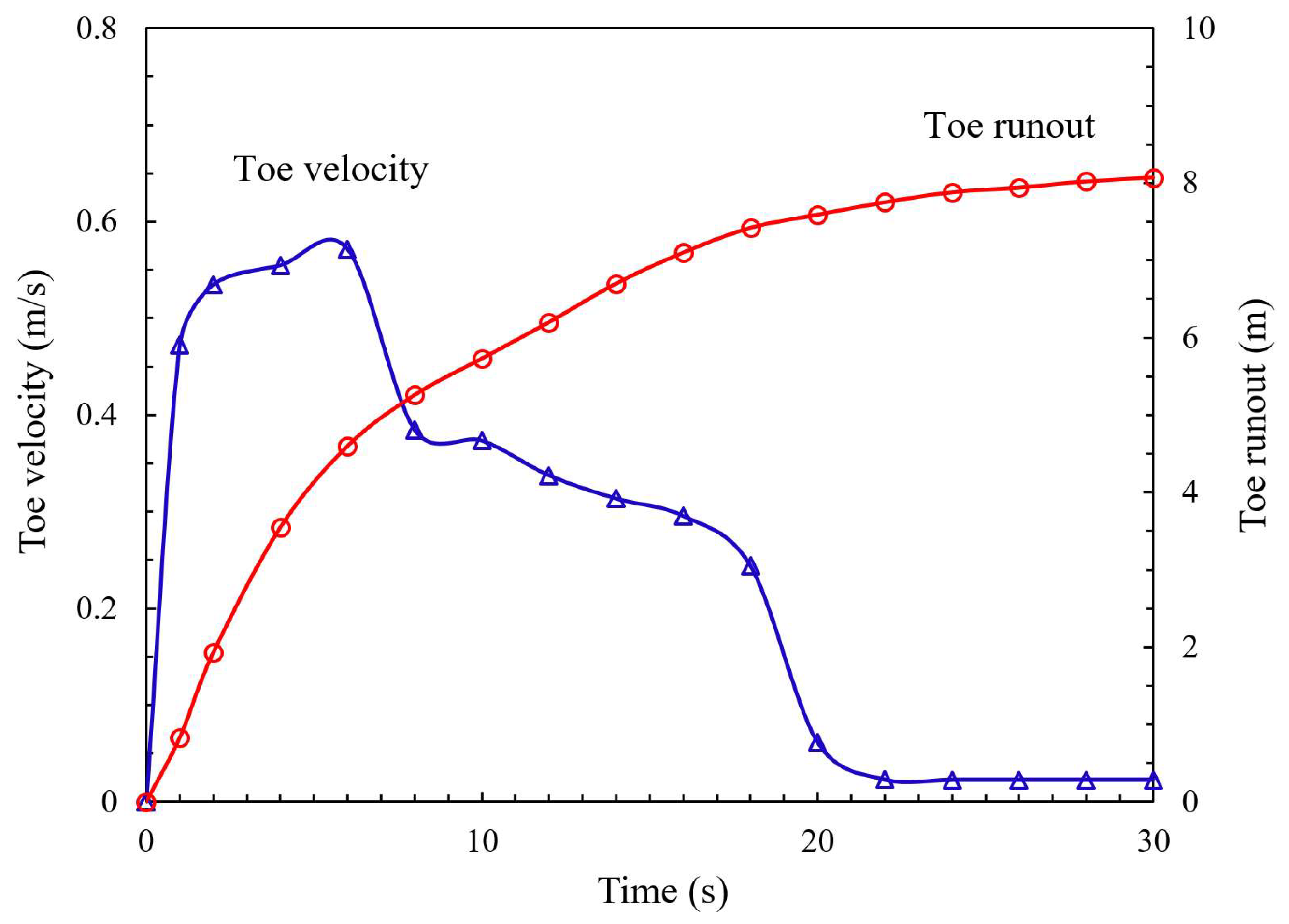
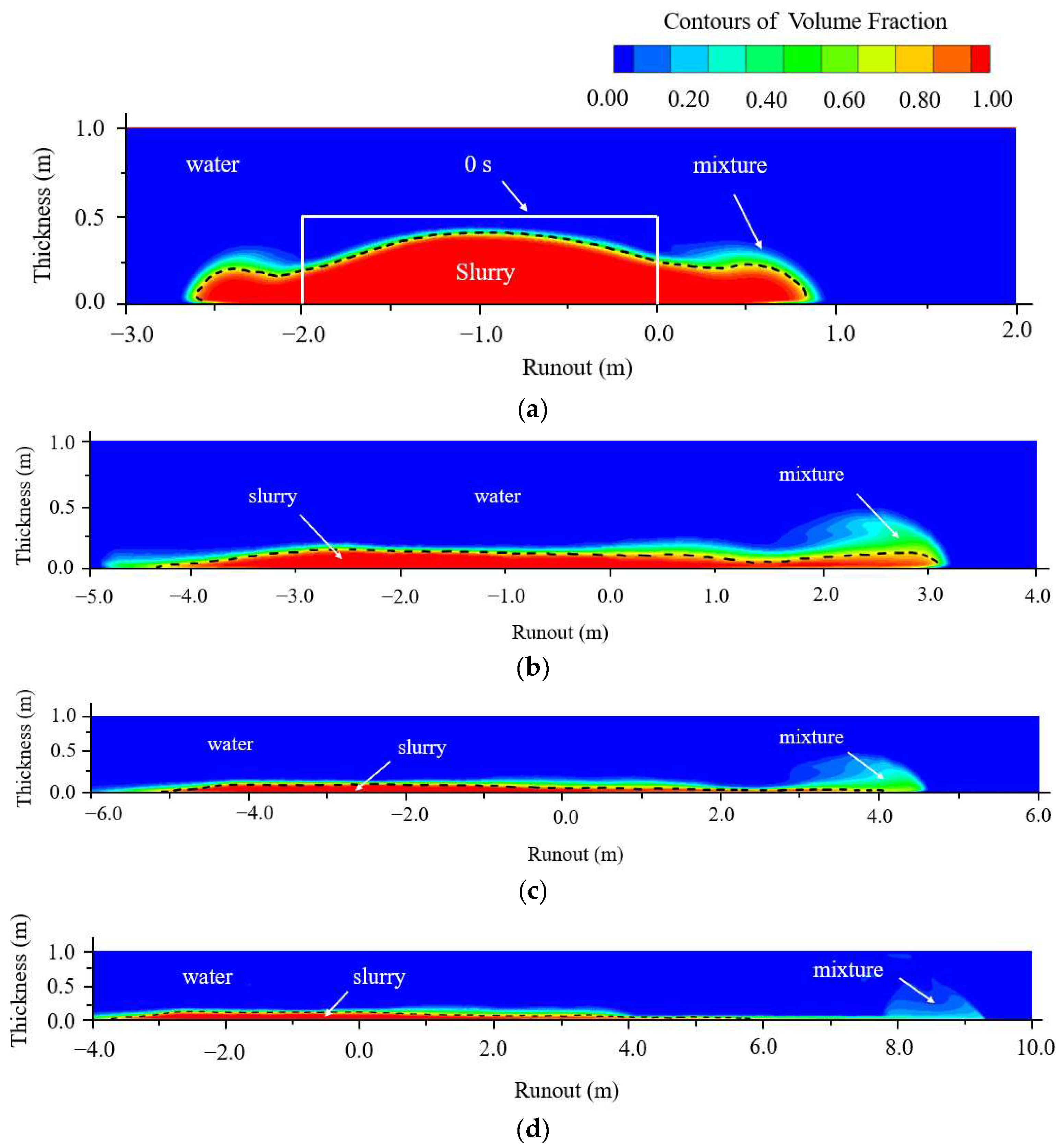
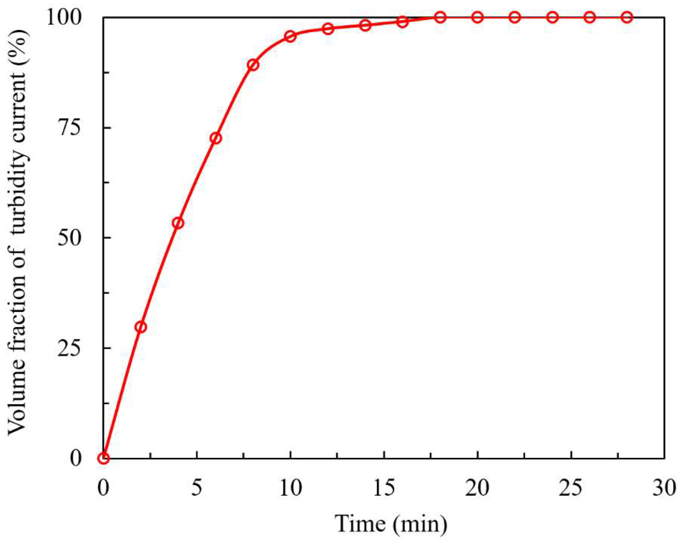
4.2. Modelling of the Transformation Process

The case with 25% clay slurry was simulated first. The velocity and the run-out distance at the toe of the slurry front are presented in Figure 5. In the run-out process, the maximum velocity at the leading edge of the slurry reaches 0.6 m/s in 6 s. Then, the velocity decreases due to the frictional resistance along the interface between the slurry bed and slurry wall. The velocity contour of the run-out at 6 s is shown in Figure 6. Due to the difference between the velocity of the front section and that of the rear section, the thickness of the slurry is continuously reduced during the run-out process, together with its elongation [56]. The body of the slurry interacts with the ambient water. As described above, shearing mainly occurs on the upper front surface between the slurry and the ambient water, as shown in Figure 7. Due to the difference between the velocity of the slurry and that of the ambient water at the stagnation point, shearing occurs at the stagnation point. The shearing force gradually erodes the slurry material from the front to the upper surface. In this process, there is continuous mixing of the eroded slurry and the ambient water, shaping a wake zone with a volume fraction ranging from nil and unity. Based on its definition, the volume fraction of a turbidity current is usually below 0.3. Thus, the transformation ratio T of the debris flow to the turbidity current can be estimated as follows:

T = A_0.3/A,

(11)

where A_0.3 and A are the areas with volume fractions smaller than 0.3 and unity, respectively. The change in the transformation ratio T as a function of time throughout the whole process is presented in Figure 8. The volume fraction of the transformed turbidity current increases in the first 6 s, reaching a maximum value of 40%. The remaining 60% of the original slurry is deposited after 6 s, as seen in Figure 8. The front parts of the slurry with higher migration velocities are almost entirely transformed. In the transformation process, the generated turbidity current with a smaller density is entrained into the ambient water and gradually diffused, as shown in Figure 9.

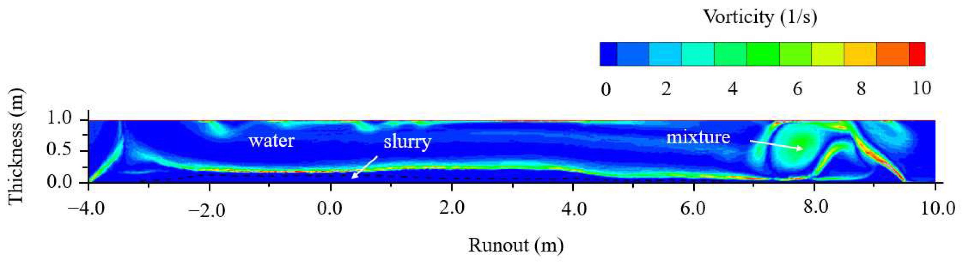
4.3. Shearing Mechanism

The shear stress on the upper surface of the debris flow can be estimated as follows [33]:

$$\tau =\frac{1}{2}{C}_{\mathrm{D}}\rho v^2$$

(12)

where τ indicates the shear stress, C_D denotes the drag coefficient, ρ represents the density of the mixture, and v denotes the velocity of the debris flow. As shown in Figure 6, at 6 s, Δv, representing the variance between the velocity of the debris flow and that of the ambient water, is approximately 0.4 m/s. The drag coefficient C_D, suggested by Norem et al. [57] and Harbitz [58] to be within the range of 0.0015 to 0.007, is chosen as 0.0015 in this study. The density of the mixture is considered to be 1500 kg/m³. Using Equation (12), the shear stress on the upper surface is calculated to be approximately 0.18 Pa.

On the other hand, the shear stress on the upper surface of the debris flow can be determined from the simulation results. The shear strain rate at 6 s, with the mixture model, increases with the mixing of the slurry and ambient water, as shown in Figure 10a. Therefore, the interface shear strain rate can be better illustrated by the counterpart results from the VOF model, as shown in Figure 10b, in which the maximum shear strain rate at the interface between the slurry and the water is approximately 100 s⁻¹. Then, the shear stress can be calculated by multiplying the shear strain rate with the viscosity of water, as τ = 100 × 0.0013 = 0.13 Pa, which is very close to that calculated from the drag force. Therefore, the shearing mechanism of the transformation from debris flows into turbidity currents is validated. Below, Equation (12) is adopted to quantify the interface shear stresses between the soil and water during shearing.

5. Parametric Studies

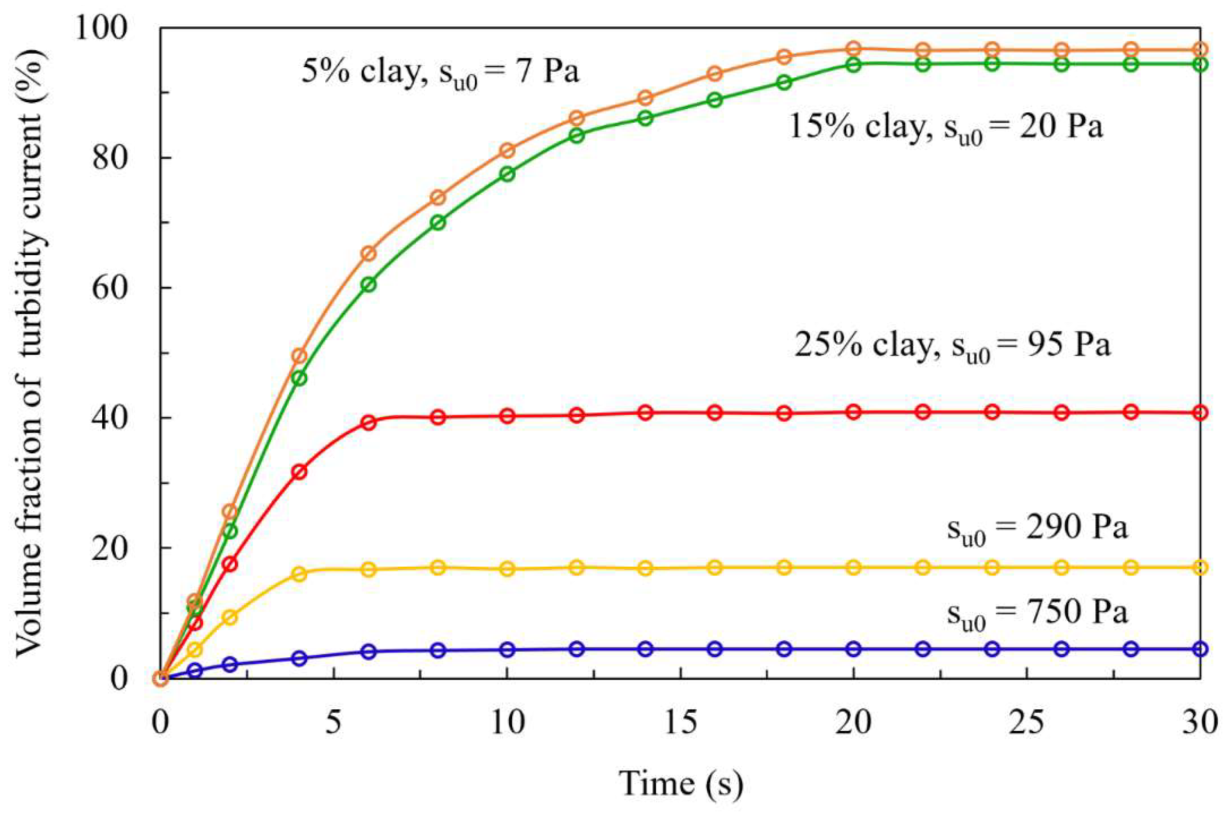
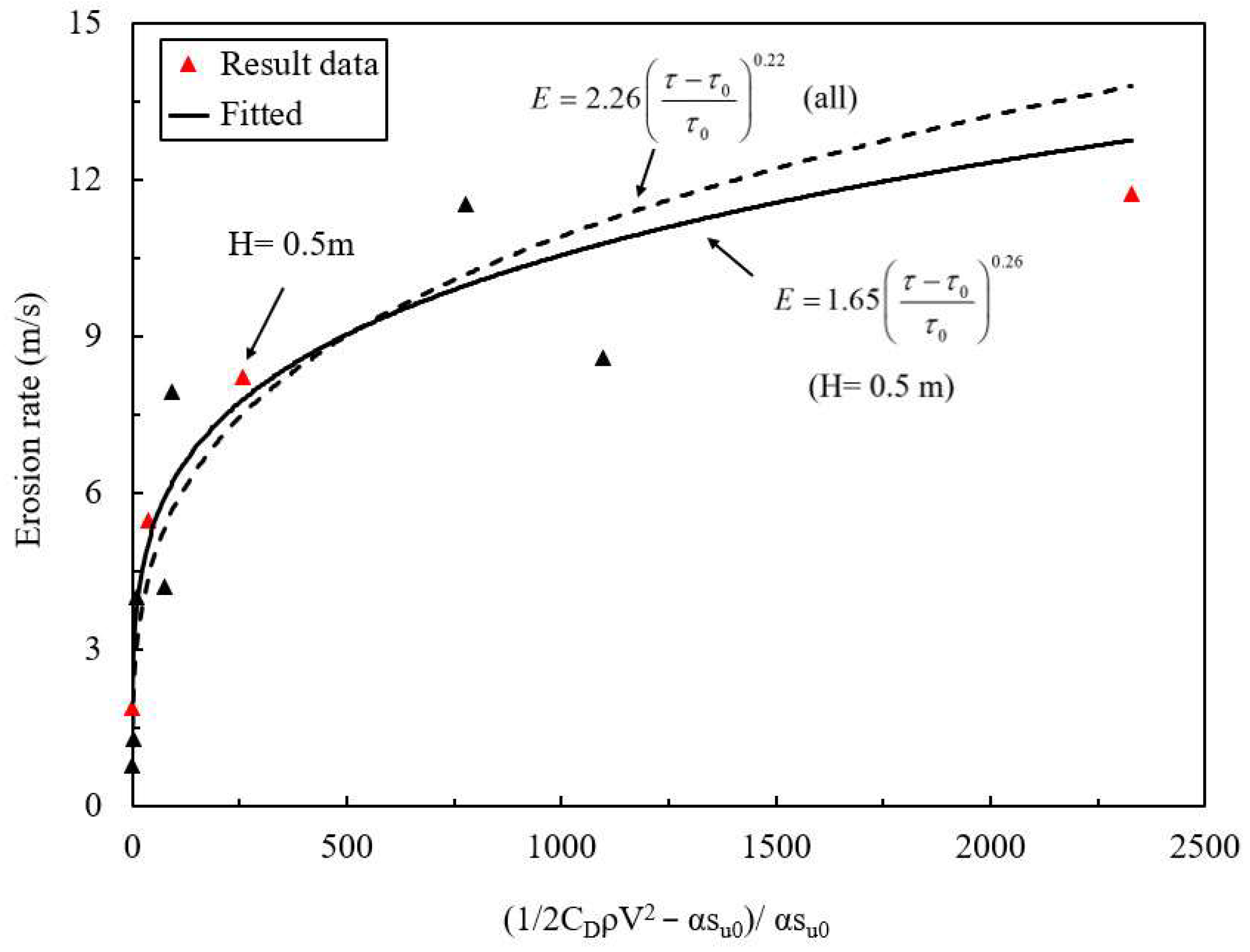
5.1. Shear Strength of the Debris Flow

The cases with 5% and 15% clay slurry were also simulated together with another case, in which the yield stress of the slurry is s_u0,H = 750 Pa and the coefficients are μ = 0.17 and n = 1.31. The variations in the transformation ratio T with time in these cases are shown in Figure 8, which indicates that the transformation ratio decreases as the yield stress of the debris flow increases. This is consistent with the findings of Huang et al. [12] and Liu et al. [13]. Herein, the transformation process is considered to be equivalent to shearing-induced erosion actions. In the existing literature, the erosion/transformation rate E of the gravity flow is usually expressed as follows:

$$E=M\left(\frac{\tau -{\tau }_0}{{\tau }_0}\right)$$

(13)

where M is a coefficient, τ is the interface shear stress between the slurry and water and can be calculated using Equation (12) and τ₀ is the minimum value of τ required for erosion/transformation to occur. To quantify the values of τ₀ in different cases, the starting time t₀ of the transformation is determined, as shown in Figure 11a. Then, the frontal velocity of the debris flow at the initial time t₀ is also extracted, and the values of τ₀ can be calculated using Equation (12). The relationship between τ₀ and the yield stress of the debris flow, as presented in Figure 11b, is observed to be linear as follows:

$${\tau }_0=\alpha s_{\mathrm{u}0}$$

(14)

where α is the coefficient and is best fitted as 6.55 × 10⁻⁵ in the above cases, with an initial slurry thickness of H = 0.5 m. The transformation rate E is extracted from Figure 8 as E = T_{(4 s)}/4, where T_{(4 s)} is the transformed volume at 4 s. Then, the data are best fitted with Equation (13), as shown in Figure 12, where the velocity v is chosen as the value at 4 s. Finally, the coefficient M and the power index n are determined as 1.61 and 0.26, respectively.

5.2. Slope Angle and Flow Depth

To explore the influences of the flow depth H and slope angle θ on the transformation rate E [59], more cases were simulated with a slope angle θ of 1° and flow depths H of 0.3 m and 0.8 m, respectively. In each of these cases, different values of the yield strength of the slurry, including 7 Pa, 20 Pa, 95 Pa, 290 Pa and 750 Pa, are considered. The simulation results show that the transformation process of the debris flow is slightly affected by the flow depth and the slope angle. The transformation rates at the initial moments are shown in Table 1. With all the data collected from these cases, Figure 11 and Figure 12 were re-drawn and the equations were updated as follows:

$${\tau }_0=5.84 \times { 10}^{-5}{s}_{\mathrm{u}0}$$

(15)

$$E=2.26{\left(\frac{\tau -{\tau }_0}{{\tau }_0}\right)}^{0.22}$$

(16)

Equations (15) and (16) were utilized to evaluate the rates of transformation of debris flows into turbidity currents.

Table 1. Transformation rates for different cases at initial moments.

Case	Slope Angle θ (°)	Initial Thickness H (m)	Yield Strength su0 (Pa)	Transformation Rate E (m/s)	Representative Velocity v (m/s)
1	6	0.3	7	8.29	1.02
2	6	0.3	20	8.08	0.79
3	6	0.3	95	4.38	0.42
4	6	0.3	290	1.33	0.13
5	6	0.3	750	0.25	0.02
6	6	0.5	7	12.38	1.53
7	6	0.5	20	11.53	1.04
8	6	0.5	95	7.93	0.56
9	6	0.5	290	4	0.34
10	6	0.5	750	0.78	0.09
11	6	0.8	7	13.84	1.86
12	6	0.8	20	12.42	1.76
13	6	0.8	95	8.69	1.27
14	6	0.8	290	5.03	0.77
15	6	0.8	750	1.95	0.28
16	1	0.5	7	10.68	0.72
17	1	0.5	20	10.03	0.68
18	1	0.5	95	6.58	0.43
19	1	0.5	290	3.53	0.17
20	1	0.5	750	0.65	0.05

Table 1. Transformation rates for different cases at initial moments.

Case	Slope Angle θ (°)	Initial Thickness H (m)	Yield Strength su0 (Pa)	Transformation Rate E (m/s)	Representative Velocity v (m/s)
1	6	0.3	7	8.29	1.02
2	6	0.3	20	8.08	0.79
3	6	0.3	95	4.38	0.42
4	6	0.3	290	1.33	0.13
5	6	0.3	750	0.25	0.02
6	6	0.5	7	12.38	1.53
7	6	0.5	20	11.53	1.04
8	6	0.5	95	7.93	0.56
9	6	0.5	290	4	0.34
10	6	0.5	750	0.78	0.09
11	6	0.8	7	13.84	1.86
12	6	0.8	20	12.42	1.76
13	6	0.8	95	8.69	1.27
14	6	0.8	290	5.03	0.77
15	6	0.8	750	1.95	0.28
16	1	0.5	7	10.68	0.72
17	1	0.5	20	10.03	0.68
18	1	0.5	95	6.58	0.43
19	1	0.5	290	3.53	0.17
20	1	0.5	750	0.65	0.05

5.3. Real-Scale Modelling

Finally, the transformation of debris flows into turbidity currents on the field scale is considered here. A computational domain of 50 km × 1 km is generated to perform the two-dimensional simulation. A uniform grid with an element size of 15 m × 15 m is used for meshing, and the entire domain of interest is meshed with 200,049 quadrilateral elements. Through trial calculations, the mesh is determined to be sufficiently fine. The initial length and thickness of the slurry are set as 3000 m and 200 m, respectively. The slurry, with an initially rectangular shape, starts to accelerate due to gravity on a slope with an angle of 1°. After 30 km, the slope angle suddenly decreases to zero. The mixture model is used as the multi-phase flow model, while the laminar model is adopted as the viscosity model. The density and the yield stress of the slurry are considered to be 1.6 × 10³ kg/m³ and 500 Pa, respectively. The viscosity of the water is 0.001 Pa·s. Pressure inlet and outlet conditions are imposed on the left wall and the right wall, respectively, while a no-slip condition is applied to the base.

The velocity and the run-out distance at the toe of the slurry front are presented in Figure 13. In the run-out process, the maximum velocity reaches 25 m/s in 4 min at the toe of the slurry front. Then, the velocity decreases due to frictional resistance along the interface between the slurry and the bed. The corresponding final run-out distance is 42.5 km. In the transportation process, the variation in the transformation ratio T with time throughout the whole process is presented in Figure 14. The debris flow is fully transformed into a turbidity current in 17.5 s, which is in accordance with the field observations. This indicates that the turbidity current can move over a longer distance than the parent debris flow.

6. Conclusions

Numerical experiments were carried out using the computational fluid dynamics method to investigate the processes of transformation from debris flows into turbidity currents during the transportation of submarine landslides. The two-phase mixture module was adopted to mimic the interactions between the slurry and the ambient water, which we validated through a dam-break case. In the numerical models, slurries with different clay contents were considered, and their rheological behaviors were characterized using the Herschel–Bulkley model. To examine the effects of the initial slurry thickness, shear strength, slope angle and flow depth on the fluid conversion, sensitivity analyses were also conducted.

Based on the multiphase flow theory and numerical simulations, it was found that the shearing effect on the transformation of debris flows into turbidity currents and the process of mixture between them can be effectively captured by the two-phase mixture module. The shear stress on the upper surface of the debris flow can be estimated by Equation (12) with the drag coefficient varied between 0.0015 and 0.007. The shearing mechanism of the transformation from debris flows into turbidity currents was validated by comparing the shear stress on the upper surface of the debris flow calculated from the numerical and theoretical methods.

A formula for the transformation rates was best fitted through a case series of debris flows. In particular, the activation stress was derived from the cases as a coefficient times the threshold shear strength of the debris, where the coefficient was estimated as 6.55 × 10⁻⁵. Similarly, the other two coefficients in the formula, i.e., the coefficient M and the power index n, were determined as 1.61 and 0.26, respectively. Finally, in a real-scale debris flow case study, we found that the slurry was fully transformed before it was deposited.

Based on the above analysis, the shearing theory behind the transformation from the debris flow to the turbidity current is unveiled. The expected outcome, the mechanical theory, the activation stress and the transformation rate would be applied to assess the influence area of the realistic turbidity currents and their harm to the subsea environment.

There are six mechanisms for the transformation from debris flow to turbidity currents as described in Felix and Peakall [21]. In future studies, quantitative analysis is expected to be conducted for each transformation mechanism to investigate the transformation efficiency under different underwater environments. The hazards caused by the submarine landslides could be better understood, based on which more reasonable mitigation measures could be proposed.

References

1. Sun, Q.; Wang, Q.; Shi, F.; Alves, T.; Gao, S.; Xie, X.; Wu, S.; Li, J. Runup of landslide-generated tsunamis controlled by paleogeography and sea-level change. Commun. Earth Environ. 2022, 3, 244. [Google Scholar] [CrossRef]
2. Talling, P.J.; Paull, C.K.; Piper, D.J. How are subaqueous sediment density flows triggered, what is their internal structure and how does it evolve? Direct observations from monitoring of active flows. Earth-Sci. Rev. 2013, 125, 244–287. [Google Scholar] [CrossRef] [Green Version]
3. Dong, Y.; Wang, D.; Randolph, M.F. Investigation of impact forces on pipeline by submarine landslide using material point method. Ocean Eng. 2017, 146, 21–28. [Google Scholar] [CrossRef]
4. Dong, Y.; Wang, D.; Cui, L. Assessment of depth-averaged method in analysing runout of submarine landslide. Landslides 2020, 17, 543–555. [Google Scholar] [CrossRef]
5. Meiburg, E.; Kneller, B. Turbidity currents and their deposits. Annu. Rev. Fluid Mech. 2010, 42, 135–156. [Google Scholar] [CrossRef] [Green Version]
6. Locat, J.; Lee, H.J. Submarine landslides: Advances and challenges. Can. Geotech. J. 2002, 39, 193–212. [Google Scholar] [CrossRef]
7. Zhang, W. Initiation and Mechanisms of Catastrophic Submarine Landslides. Ph.D. Thesis, The University of Western Australia, Perth, Australia, 2017. [Google Scholar]
8. Guo, X.-S.; Nian, T.-K.; Gu, Z.-D.; Li, D.-Y.; Fan, N.; Zheng, D.-F. Evaluation methodology of laminar-turbulent flow state for fluidized material with special reference to submarine landslide. J. Waterw. Port Coast. Ocean Eng. 2021, 147, 04020048. [Google Scholar] [CrossRef]
9. Elverhøi, A.; Harbitz, C.B.; Dimakis, P.; Mohrig, D.; Marr, J.; Parker, G. On the dynamics of subaqueous debris flows. Oceanography 2000, 13, 109–117. [Google Scholar] [CrossRef]
10. Boukpeti, N.; White, D.; Randolph, M.; Low, H. Strength of fine-grained soils at the solid–fluid transition. Géotechnique 2012, 62, 213–226. [Google Scholar] [CrossRef] [Green Version]
11. Mohrig, D.; Ellis, C.; Parker, G.; Whipple, K.X.; Hondzo, M. Hydroplaning of subaqueous debris flows. Geol. Soc. Am. Bull. 1998, 110, 387–394. [Google Scholar] [CrossRef]
12. Huang, H.; Imran, J.; Pirmez, C. Numerical study of turbidity currents with sudden-release and sustained-inflow mechanisms. J. Hydraul. Eng. 2008, 134, 1199–1209. [Google Scholar] [CrossRef]
13. Liu, D.; Cui, Y.; Guo, J.; Yu, Z.; Chan, D.; Lei, M. Investigating the effects of clay/sand content on depositional mechanisms of submarine debris flows through physical and numerical modeling. Landslides 2020, 17, 1863–1880. [Google Scholar] [CrossRef]
14. Wells, M.G.; Dorrell, R.M. Turbulence processes within turbidity currents. Annu. Rev. Fluid Mech. 2021, 53, 59–83. [Google Scholar] [CrossRef]
15. Xie, X.; Tian, Y.; Wei, G. Deduction of sudden rainstorm scenarios: Integrating decision makers’ emotions, dynamic Bayesian network and DS evidence theory. Nat. Hazards 2022. [Google Scholar] [CrossRef]
16. Mulder, T.; Cochonat, P. Classification of offshore mass movements. J. Sediment. Res. 1996, 66, 43–57. [Google Scholar]
17. Nian, T.-K.; Guo, X.-S.; Zheng, D.-F.; Xiu, Z.-X.; Jiang, Z.-B. Susceptibility assessment of regional submarine landslides triggered by seismic actions. Appl. Ocean Res. 2019, 93, 101964. [Google Scholar] [CrossRef]
18. Hampton, M.A. The role of subaqueous debris flow in generating turbidity currents. J. Sediment. Res. 1972, 42, 775–793. [Google Scholar]
19. Zhu, X.; Xu, Z.; Liu, Z.; Liu, M.; Yin, Z.; Yin, L.; Zheng, W. Impact of dam construction on precipitation: A regional perspective. In Marine and Freshwater Research; CSIRO Publishing: Melbourne, Australia, 2022. [Google Scholar]
20. Khorasani, M.; Ghasemi, A.; Leary, M.; Sharabian, E.; Cordova, L.; Gibson, I.; Downing, D.; Bateman, S.; Brandt, M.; Rolfe, B. The effect of absorption ratio on meltpool features in laser-based powder bed fusion of IN718. Opt. Laser Technol. 2022, 153, 108263. [Google Scholar] [CrossRef]
21. Felix, M.; Peakall, J. Transformation of debris flows into turbidity currents: Mechanisms inferred from laboratory experiments. Sedimentology 2006, 53, 107–123. [Google Scholar] [CrossRef]
22. Mohrig, D.; Marr, J.G. Constraining the efficiency of turbidity current generation from submarine debris flows and slides using laboratory experiments. Mar. Pet. Geol. 2003, 20, 883–899. [Google Scholar] [CrossRef]
23. Yuan, J.; Gan, Y.; Chen, J.; Tan, S.; Zhao, J. Experimental research on consolidation creep characteristics and microstructure evolution of soft soil. Front. Mater. 2023, 10, 70. [Google Scholar] [CrossRef]
24. Kuenen, P.H.; Migliorini, C. Turbidity currents as a cause of graded bedding. J. Geol. 1950, 58, 91–127. [Google Scholar] [CrossRef]
25. Kuenen, P.H. Estimated size of the Grand Banks [Newfoundland] turbidity current. Am. J. Sci. 1952, 250, 874–884. [Google Scholar] [CrossRef]
26. Chand, R.; Sharma, V.S.; Trehan, R.; Gupta, M.K. Numerical investigations on mechanical properties of bio-inspired 3D printed geometries using multi-jet fusion process. Rapid Prototyp. J. 2023. ahead-of-print. [Google Scholar] [CrossRef]
27. Zhang, C.; Yin, Y.; Yan, H.; Zhu, S.; Li, B.; Hou, X.; Yang, Y. Centrifuge modeling of multi-row stabilizing piles reinforced reservoir landslide with different row spacings. Landslides 2023, 20, 559–577. [Google Scholar] [CrossRef]
28. Morgenstern, N. Submarine slumping and the initiation of turbidity currents. Mar. Geotech. 1967, 3, 189–220. [Google Scholar]
29. Allen, J. Mixing at turbidity current heads, and its geological implications. J. Sediment. Res. 1971, 41, 97–113. [Google Scholar]
30. Xie, X.; Xie, B.; Cheng, J.; Chu, Q.; Dooling, T. A simple Monte Carlo method for estimating the chance of a cyclone impact. Nat. Hazards 2021, 107, 2573–2582. [Google Scholar] [CrossRef]
31. Van Andel, T.H.; Komar, P.D. Ponded sediments of the Mid-Atlantic Ridge between 22 and 23 North latitude. Geol. Soc. Am. Bull. 1969, 80, 1163–1190. [Google Scholar] [CrossRef]
32. Dangeard, L.; Larsonneur, C.; Migniot, C. Les courants de turbidité, les coulées boueuses et les glissements: Résultats d’expériences. C R de L’académie Des. Sci. Paris 1965, 261, 2123–2127. [Google Scholar]
33. Talling, P.; Peakall, J.; Sparks, R.; Cofaigh, Ó.C.; Dowdeswell, J.; Felix, M.; Wynn, R.; Baas, J.; Hogg, A.; Masson, D. Experimental constraints on shear mixing rates and processes: Implications for the dilution of submarine debris flows. Geol. Soc. Lond. Spec. Publ. 2002, 203, 89–103. [Google Scholar] [CrossRef]
34. Bradford, S.F.; Katopodes, N.D. Hydrodynamics of turbid underflows. I: Formulation and numerical analysis. J. Hydraul. Eng. 1999, 125, 1006–1015. [Google Scholar] [CrossRef]
35. Zhu, H.; Randolph, M.F. Large deformation finite-element analysis of submarine landslide interaction with embedded pipelines. Int. J. Geomech. 2010, 10, 145–152. [Google Scholar] [CrossRef]
36. Medina, V.; Hürlimann, M.; Bateman, A. Application of FLATModel, a 2D finite volume code, to debris flows in the northeastern part of the Iberian Peninsula. Landslides 2008, 5, 127–142. [Google Scholar] [CrossRef]
37. Wang, Z.; Li, X.; Liu, P.; Tao, Y. Numerical analysis of submarine landslides using a smoothed particle hydrodynamics depth integral model. Acta Oceanol. Sin. 2016, 35, 134–140. [Google Scholar] [CrossRef]
38. Heinrich, P. Nonlinear water waves generated by submarine and aerial landslides. J. Waterw. Port Coast. Ocean Eng. 1992, 118, 249–266. [Google Scholar] [CrossRef]
39. Abe, K.; Soga, K.; Bandara, S. Material point method for coupled hydromechanical problems. J. Geotech. Geoenviron. Eng. 2014, 140, 04013033. [Google Scholar] [CrossRef]
40. Maury, B. Characteristics ALE method for the unsteady 3D Navier-Stokes equations with a free surface. Int. J. Comput. Fluid Dyn. 1996, 6, 175–188. [Google Scholar] [CrossRef]
41. Basting, S.; Quaini, A.; Čanić, S.; Glowinski, R. Extended ALE method for fluid–structure interaction problems with large structural displacements. J. Comput. Phys. 2017, 331, 312–336. [Google Scholar] [CrossRef] [Green Version]
42. Hirt, C.W.; Nichols, B.D. Volume of fluid (VOF) method for the dynamics of free boundaries. J. Comput. Phys. 1981, 39, 201–225. [Google Scholar] [CrossRef]
43. Zhou, L.; Sun, J. Integrated ecosystem management and regulation strategies in the South China Sea. J. Sea Res. 2022, 190, 102300. [Google Scholar] [CrossRef]
44. Zhou, G.; Li, W.; Zhou, X.; Tan, Y.; Lin, G.; Li, X.; Deng, R. An innovative echo detection system with STM32 gated and PMT adjustable gain for airborne LiDAR. Int. J. Remote Sens. 2021, 42, 9187–9211. [Google Scholar] [CrossRef]
45. Liu, Y.; Zhang, K.; Li, Z.; Liu, Z.; Wang, J.; Huang, P. A hybrid runoff generation modelling framework based on spatial combination of three runoff generation schemes for semi-humid and semi-arid watersheds. J. Hydrol. 2020, 590, 125440. [Google Scholar] [CrossRef]
46. Marr, J.G.; Elverhøi, A.; Harbitz, C.; Imran, J.; Harff, P. Numerical simulation of mud-rich subaqueous debris flows on the glacially active margins of the Svalbard–Barents Sea. Mar. Geol. 2002, 188, 351–364. [Google Scholar] [CrossRef]
47. Zakeri, A.; Høeg, K.; Nadim, F. Submarine debris flow impact on pipelines—Part I: Experimental investigation. Coast. Eng. 2008, 55, 1209–1218. [Google Scholar] [CrossRef]
48. Marr, J.G.; Harff, P.A.; Shanmugam, G.; Parker, G. Experiments on subaqueous sandy gravity flows: The role of clay and water content in flow dynamics and depositional structures. Geol. Soc. Am. Bull. 2001, 113, 1377–1386. [Google Scholar] [CrossRef]
49. De Blasio, F.V.; Engvik, L.; Harbitz, C.B.; Elverhøi, A. Hydroplaning and submarine debris flows. J. Geophys. Res. Ocean. 2004, 109, C01002. [Google Scholar] [CrossRef]
50. Wu, J.; Long, J.; Liu, M. Evolving RBF neural networks for rainfall prediction using hybrid particle swarm optimization and genetic algorithm. Neurocomputing 2015, 148, 136–142. [Google Scholar] [CrossRef]
51. Ghahramani-Wright, V. Laboratory and Numerical Study of Mud and Debris Flow; University of California: Davis, CA, USA, 1987; Volumes I and II. [Google Scholar]
52. Dong, Y.; Cui, L.; Zhang, X. Multiple-GPU parallelization of three-dimensional material point method based on single-root complex. Int. J. Numer. Methods Eng. 2022, 123, 1481–1504. [Google Scholar] [CrossRef]
53. Elverhoi, A.; Breien, H.; De Blasio, F.V.; Harbitz, C.B.; Pagliardi, M. Submarine landslides and the importance of the initial sediment composition for run-out length and final deposit. Ocean Dyn. 2010, 60, 1027–1046. [Google Scholar] [CrossRef] [Green Version]
54. Graziosi, S.; Ballo, F.M.; Libonati, F.; Senna, S. 3D printing of bending-dominated soft lattices: Numerical and experimental assessment. Rapid Prototyp. J. 2022, 28, 51–64. [Google Scholar]
55. Dong, Y.; Liao, Z.; Wang, J.; Liu, Q.; Cui, L. Potential failure patterns of a large landslide complex in the Three Gorges Reservoir area. Bull. Eng. Geol. Environ. 2023, 82, 1–20. [Google Scholar] [CrossRef]
56. Xu, J.; Lan, W.; Ren, C.; Zhou, X.; Wang, S.; Yuan, J. Modeling of coupled transfer of water, heat and solute in saline loess considering sodium sulfate crystallization. Cold Reg. Sci. Technol. 2021, 189, 103335. [Google Scholar] [CrossRef]
57. Norem, H.; Locat, J.; Schieldrop, B. An approach to the physics and the modeling of submarine flowslides. Mar. Georesour. Geotechnol. 1990, 9, 93–111. [Google Scholar] [CrossRef]
58. Harbitz, C. Model simulations of tsunamis generated by the Storegga slides. Mar. Geol. 1992, 105, 1–21. [Google Scholar] [CrossRef]
59. Wu, Z.; Xu, J.; Li, Y.; Wang, S. Disturbed state concept–based model for the uniaxial strain-softening behavior of fiber-reinforced soil. Int. J. Geomech. 2022, 22, 04022092. [Google Scholar] [CrossRef]
Figure 1. Evolution process of a submarine landslide (adapted with permission from Ref. [8]. 2021, Xing-sen Guo).
Applsci 13 04105 g001
Figure 2. Transformation of the debris flow into the turbidity current.
Applsci 13 04105 g002
Figure 3. Simulation of the dam break case with the multi-phase framework. (a) Initial geometry of the dam break case (not to scale); (b) Runout profile at 4.1 s.
Applsci 13 04105 g003
Figure 5. Changes in the velocity and run-out distance as a function of time during the run-out process.
Applsci 13 04105 g005
Figure 6. Velocity contour of the slurry at 6 s.
Applsci 13 04105 g006
Figure 7. Volume fraction contours of the slurry at different points in time. (a) 1s. (b) 3.5 s. (c) 6 s. (d) 15 s.
Applsci 13 04105 g007
Figure 8. Change in the transformation ratio of the debris flow as a function of time.
Applsci 13 04105 g008
Figure 9. Vorticity contour at 15 s.
Applsci 13 04105 g009
Figure 10. Shear strain rate contour at 6 s. (a) The mixture model. (b) The VOF model.
Applsci 13 04105 g010
Figure 11. Determination of the activation shear stress. (a) Transformation at initial moments; (b) Best-fit of the activation shear stress.
Applsci 13 04105 g011aApplsci 13 04105 g011b
Figure 12. Relationship between the erosion rate and the flow velocity.
Applsci 13 04105 g012
Figure 13. Changes in the velocity and run-out distance of the real-scale case as a function of time.
Applsci 13 04105 g013
Figure 14. Change in the transformation ratio T throughout the whole process.
Applsci 13 04105 g014
Disclaimer/Publisher’s Note: The statements, opinions and data contained in all publications are solely those of the individual author(s) and contributor(s) and not of MDPI and/or the editor(s). MDPI and/or the editor(s) disclaim responsibility for any injury to people or property resulting from any ideas, methods, instructions or products referred to in the content.