Vertical Seismic-Profile Data Local Full-Waveform Inversion Based on Marchenko Redatuming

Abstract

Local full-waveform inversion (FWI) methods use redatumed seismic responses of virtual receivers within the subsurface to build the local objective function based on the convolution-type representation theorem. The Marchenko method is widely used to obtain the redatumed data. The method only requires a smoothed velocity model with correct kinematic characteristics of seismic responses for redatuming of the single-sided reflection data. However, the standard Marchenko method is insensitive to lateral propagation of the wavefield. By injecting the standard Marchenko redatumed wavefield along the boundary of the target, the local wavefield propagation modeling produces errors, which affects the accuracy of the local FWI. In this paper, a method to obtain more accurate Green’s functions is proposed by incorporating vertical seismic profile data (VSP) into the calculation process of the Marchenko source-receiver redatuming. This method allows one to obtain the accurate laterally propagating waveform, resulting in a significant improvement of lateral resolution. The proposed method is applied to a benchmark model dataset and compared with the local FWI based on standard Marchenko redatuming.

1. Introduction

The inversion of seismic data is one of the most effective methods to characterize reservoirs. In general, the conventional input for wave impedance inversion is a post-stack seismic profile or seismic volume, which assumes that all diffracted energy has been focused on the diffracted object by the migration process [1]. In practice, inaccuracies in the velocity model are common, leading to conflicts with that assumption. The seismic responses corresponding to small-scale reservoirs (like caves, faults, and fractures) with high heterogeneous patterns are mainly generated from diffraction [2,3]. These lead to the inability of conventional inversion methods to correctly characterize these small-scale reservoirs. How to make sensible use of seismic full waveform information is the key to inversion of these complex reservoirs.

Tarantola (1984) proposed a generalized least squares-based full waveform inversion (FWI) method in the time domain [4,5]. The method reconstructs the model parameters by analyzing the complete seismic waveforms (including amplitudes and travel times). With the high accuracy of the inverted model reconstructed by FWI and the enhanced computational power, the FWI method has become a focal area in current geophysical research. Pratt (1999) proposed the frequency-domain FWI method which directly performs inversion for various frequency components. Compared with time-domain inversion, frequency-domain FWI makes multiscale inversion more convenient. Generally, in the frequency domain, the multiscale approach is implemented by the successive inversion of single frequencies or groups of selected frequencies from low to high [6,7,8]. High-frequency FWI has the potential to recover high-resolution subsurface model parameters [8,9]. The results of this method can help in identifying fine reservoir characteristics and in interpreting complex subsurface structures. However, high-frequency FWI requires tremendous computer resources because of its small scale spatial and time sampling to ensure the stability of the wave propagating simulation [10]. However, for reservoir characterization, we are usually interested in a small range. Therefore, the inversion of the entire model is not needed. Moreover, it is difficult to perform FWI on deeply buried reservoirs under complex overburdens because the strong scattering from the overburden tends to obscure the reflections from the region of interest [11]. Target-oriented local inversion methods were developed to focus the inversion on a target area [12,13,14,15]. Yuan et al. developed a time-lapse seismic local FWI method based on the wavefield injection technique [12,13,16]. However, this method requires accurate model parameters of overburden to simulate Green’s function on the subsurface virtual receivers [12,13]. Guo and Alkhalifah obtained virtual data at a subsurface datum level by introducing a robust waveform-based redatuming approach [17]. Using the retrieved virtual data, high-resolution local FWI and time-lapse FWI are performed without overburden. Li and Alkhalifah extended the redatuming method to be adapted into elastic media [18].

Wapenaar et al. proposed the multidimensional Marchenko equations based on the one-dimensional Marchenko representation by introducing the focusing function [19,20,21,22]. The multidimensional Marchenko equations can be used for redatuming Green’s functions of the virtual receivers. This method requires only a smoothed velocity model with correct kinematic information and does not need physical sources or receivers in the subsurface medium [19,20,21,23]. By using the Marchenko redatuming method, we can obtain subsurface receiver redatumed Green’s functions along the boundary enclosing the zone in which we are interested. However, the standard Marchenko method is insensitive to lateral propagation of the wavefield under highly complex geological structures [24]. Due to the errors of the redatumed Green’s functions, it will be difficult to maintain reasonable accuracy in the local full waveform inversion [14]. Likewise, since the observations in the target-oriented FWI are also retrieved by Marchenko redatuming, this would lead to the unsatisfactory lateral resolution of the inversion results, as well as low sensitivity to steep structures [14]. In this study, we extend the local full waveform inversion using Marchenko methods with vertical seismic-profile (VSP) data to address the deficiencies in the lateral resolution and the poor reconstruction of the steep structure of local FWI method.

Singh and Snieder obtained virtual seismic data with virtual sources and receivers in the subsurface using a method called source-receiver Marchenko redatuming [25]. In their method, receiver-redatumed Green’s functions are calculated by the standard Marchenko method to redatum the source to another location in the subsurface (virtual source point). Lomas et al. extended the source-receiver Marchenko redatuming method by replacing the receiver-redatumed Green’s functions with VSP responses. The output of this method is an estimate of the wavefield from a subsurface virtual source, which potentially contains the information about lateral propagation of the wavefield. [26]. We, therefore, introduce the VSP data into Marchenko redatuming to add a new set of virtual shot records to the local FWI and reorganize the objective function.

In this paper, we first introduce the local FWI method in the frequency domain based on standard Marchenko redatuming. It includes the derivation of the local forward modeling operator and the establishment of the objective function. Then, we use the source-receiver Marchenko redatuming method with VSP data to estimate the Green’s functions of the virtual receivers (along the boundary of the target) with the virtual sources (downhole physical receivers) in the wellbore. Compared to the standard Marchenko method, the data reconstructed by the Marchenko method with VSP have a higher accuracy by accounting for the laterally propagating wavefield signals. Finally, we incorporate the retrieved wavefields into the local FWI method. The inversion results demonstrate a good improvement in the lateral resolution. The proposed method is applied to a synthetic benchmark model for a carbonate reservoir in the Tarim Basin with strike-slip faults and fracture-vuggy karsts. The FWI result verifies the effectiveness of this method.

2. Principles and Methods

2.1. Local FWI Based on Standard Marchenko Redatuming

According to waveform-matching criteria, the FWI method can be used to obtain parameters of underground media using amplitude, travel time, and phase information. The traditional frequency domain FWI objective function can be expressed as [6]:

$${\min }_{m}E(m,\omega )=\frac{1}{2}{‖\mathbb{P}A{(m,\omega )}^{-1}f(x,z,\omega )-D_{ob\mathrm{s}}(\omega )‖}_2^2.$$

(1)

where $m$ is the model parameters, $\omega$ is the angular frequency, $A$ is the impedance matrix, and $f$ is the source operator (to ensure the shot locations and amplitude energy). $D_{ob\mathrm{s}}$ is the observed seismic data and $\mathbb{P}$ is the receiver vector (to ensure the receiver location corresponds to the observed data). In the subsequent part, the spatial coordinates $x$ and $z$ will be implicitly included in the subsequent equations.

In frequency domain FWI, the objective function is the functional under the L2 norm, which can be solved using the adjoint state method [27]:

$$\delta E={\omega }^{2}diag{(u)}^{*}v.$$

(2)

where $u$ is the forward wavefield, $v$ is the adjoint wavefield and superscript symbol * means complex conjugate. This means that we have to solve the following forward modeling equations iteratively at each frequency or frequency group:

$$A(m)u=f,$$

(3)

and

$$A{(m)}^{*}v={\mathbb{P}}^T(\mathbb{P}u-D_{obs}).$$

(4)

Under the conditions of a complete full-domain model, $A$ is usually an enormously sparse matrix. The method, therefore, has high computational requirements and low computational efficiency, especially in high frequency because fine spatial sampling intervals are required to stabilize the wavefield simulations. When only a small area in the subsurface is the target, the inversion of the entire model could be computationally very wasteful.

The finite difference wavefield injection (FD injection) method records the Green’s functions of all points on the boundary of a target and injects the background wavefield of the full model into the local region. By applying the wavefield injection method, the seismic response of the entire model can be updated by simulating only the local wavefield when only the local model parameters are changed. A source field can be introduced into a localized finite difference grid by injecting an analytical source solution along a closed surface [15]. Similarly, the wavefile recorded along a closed surface can be used as a source wavefield to compute the wavefield within the injected grid region. The main idea of FD injection is to satisfy the principles of superposition and wavefield continuity across the injection surface. That is, we can simulate only Green’s function inside the injected volume and thus obtain the wavefield of the subsurface target range corresponding to the surface source [15]. The mathematical expression of this process can be given by the convolution-type representation theorem, which we will describe below. We follow this idea and derive the local forward modeling operator in the following sections. We define the model as two computational spaces. The two computational states can be illustrated as shown in Figure 1.

The surface is represented as the black dashed line $\partial {\mathrm{D}}_s$. The dashed rectangular box $\partial {\mathrm{D}}_b$ is the boundary of the target. ${\mathrm{D}}_{in}$ is the internal region of the target zone, ${\mathrm{D}}_{out}$ is the external region. The first computational state is the complete model, containing ${\mathrm{D}}_{in}$ and ${\mathrm{D}}_{out}$. The second computational space is a truncated medium with ${\mathrm{D}}_{in}$ only. Under the first computational state, assume a point ${\mathrm{x}}_s$ at the surface as the source, then the Green’s function received by a point $\mathrm{x}$ inside ${\mathrm{D}}_{in}$ is written as $G_{all}(\mathrm{x},{\mathrm{x}}_s)$ (blue arrowed line in Figure 1). For the two-dimensional isotropic acoustic medium, the Green’s function in the frequency domain can be expressed by the second-order acoustic wave equation [28]:

$$\frac{\partial }{\partial x}[\frac{1}{\rho (\mathrm{x})}\frac{\partial }{\partial x}G(\mathrm{x},{\mathrm{x}}^{\prime },\omega )]+\frac{\partial }{\partial z}[\frac{1}{\rho (\mathrm{x})}\frac{\partial }{\partial z}G(\mathrm{x},{\mathrm{x}}^{\prime },\omega )]+{\omega }^{2}m(\mathrm{x})\frac{1}{\rho (\mathrm{x})}G(\mathrm{x},{\mathrm{x}}^{\prime },\omega )=-\iota \omega \delta (\mathrm{x}-{\mathrm{x}}^{\prime }).$$

(5)

where $m(\mathrm{x})$ is the squared slowness at point $\mathrm{x}$, $\rho$ is the density and $\iota$ is the imaginary unit. $\omega$ is the angular frequency and $G(\mathrm{x},{\mathrm{x}}^{\prime },\omega )$ denotes the Green’s function between the source ${\mathrm{x}}^{\prime }$ and the receiver point $\mathrm{x}$ at $\omega$ angular frequency. In the second computational state, only the truncated space ${\mathrm{D}}_{in}$ exists. $G_{all}(\mathrm{x},{\mathrm{x}}_s)$ can be represented by the source-free acoustic wave equation [14]:

$$\frac{\partial }{\partial x}[\frac{1}{\rho (\mathrm{x})}\frac{\partial }{\partial x}{G}_{all}(\mathrm{x},{\mathrm{x}}_s,\omega )]+\frac{\partial }{\partial z}[\frac{1}{\rho (\mathrm{x})}\frac{\partial }{\partial z}{G}_{all}(\mathrm{x},{\mathrm{x}}_s,\omega )]+{\omega }^{2}m(\mathrm{x})\frac{1}{\rho (\mathrm{x})}{G}_{all}(\mathrm{x},{\mathrm{x}}_s,\omega )=0\mathrm{x}\in {\mathrm{D}}_{in}.$$

(6)

and the Green’s function of the point source ${\mathrm{x}}_{vr}$ is noted as $G_{in}(\mathrm{x},{\mathrm{x}}_{vr})$ (red arrowed line in Figure 2), that is,

$$\frac{\partial }{\partial x}[\frac{1}{\rho (\mathrm{x})}\frac{\partial }{\partial x}{G}_{in}(\mathrm{x},{\mathrm{x}}_{vr},\omega )]+\frac{\partial }{\partial z}[\frac{1}{\rho (\mathrm{x})}\frac{\partial }{\partial z}{G}_{in}(\mathrm{x},{\mathrm{x}}_{vr},\omega )]+{\omega }^{2}m(\mathrm{x})\frac{1}{\rho (\mathrm{x})}{G}_{in}(\mathrm{x},{\mathrm{x}}_{vr},\omega )=-\iota \omega \delta (\mathrm{x}-{\mathrm{x}}_{vr})\mathrm{x}\in {\mathrm{D}}_{in}.$$

(7)

Combining Equation (6) multiplied by $G_{in}(\mathrm{x},{\mathrm{x}}_{vr})$ and Equation (7) multiplied by $G_{all}(\mathrm{x},{\mathrm{x}}_s)$, and integrating both sides of the combined equation over $D_{in}$, we have,

$$\begin{array}{cc}\hfill G_{all}({\mathrm{x}}_{vr},{\mathrm{x}}_s)=\frac{1}{\iota \omega }{\int }_{{\mathrm{D}}_{in}}& G_{in}(\mathrm{x},{\mathrm{x}}_{vr})\{\frac{\partial }{\partial x}[\frac{1}{\rho (\mathrm{x})}\frac{\partial }{\partial x}{G}_{all}(\mathrm{x},{\mathrm{x}}_s)]+\frac{\partial }{\partial z}[\frac{1}{\rho (\mathrm{x})}\frac{\partial }{\partial z}{G}_{all}(\mathrm{x},{\mathrm{x}}_s)]\}-\hfill \\ & G_{all}(\mathrm{x},{\mathrm{x}}_s)\{\frac{\partial }{\partial x}[\frac{1}{\rho (\mathrm{x})}\frac{\partial }{\partial x}{G}_{in}(\mathrm{x},{\mathrm{x}}_{vr})]+\frac{\partial }{\partial z}[\frac{1}{\rho (\mathrm{x})}\frac{\partial }{\partial z}{G}_{in}(\mathrm{x},{\mathrm{x}}_{vr})]\}d{\mathrm{x}}^2\mathrm{x}\in {\mathrm{D}}_{in}.\hfill \end{array}$$

(8)

According to the Gaussian theorem, the volume integral is equal to the enclosed boundary surface integral; then Equation (8) can be written as the functional convolution-type representation theorem [12,13,14],

$$G_{all}({\mathrm{x}}_{vr},{\mathrm{x}}_s)=\frac{1}{\iota \omega }{\oint }_{\partial {\mathrm{D}}_b}\frac{1}{\rho ({\mathrm{x}}_{vs})}[G_{in}({\mathrm{x}}_{vs},{\mathrm{x}}_{vr})\frac{\partial }{\partial n_{{\mathrm{x}}_{vs}}}{G}_{all}({\mathrm{x}}_{vs},{\mathrm{x}}_s)-\frac{\partial }{\partial n_{{\mathrm{x}}_{vs}}}{G}_{in}({\mathrm{x}}_{vs},{\mathrm{x}}_{vr})G_{all}({\mathrm{x}}_{vs},{\mathrm{x}}_s)]d{\mathrm{x}}_{vs}{\mathrm{x}}_{vs}\in \partial {\mathrm{D}}_b.$$

(9)

where ${\mathrm{x}}_{vs}$ is the virtual source point along the target area boundary $\partial {\mathrm{D}}_b$, $n_{{\mathrm{x}}_{vs}}$ is the outward unit normal to ${\mathrm{x}}_{vs}$ along the enclosed boundary $\partial {\mathrm{D}}_b$. According to the reciprocity theorem, $G_{in}({\mathrm{x}}_{vs},{\mathrm{x}}_{vr},\omega )$ is equivalent to $G_{in}({\mathrm{x}}_{vr},{\mathrm{x}}_{vs},\omega )$, while ${\mathrm{x}}_{vr}$ can be any point in the target area ${\mathrm{D}}_{in}$. Our goal is to obtain the wavefield in the target region; therefore, we replace $G_{all}({\mathrm{x}}_{vs},{\mathrm{x}}_s,\omega )$ with the wavefield represented as $P_{all}({\mathrm{x}}_{vs},{\mathrm{x}}_s,\omega )$. We can then obtain the local forward modeling operator,

$$\mathrm{F}(m_{in},\omega )=\frac{1}{\iota \omega }{\displaystyle {\oint }_{\partial {\mathrm{D}}_b}\frac{1}{\rho ({\mathrm{x}}_{vs})}[G_{in}(\mathrm{x},{\mathrm{x}}_{vs},\omega )\frac{\partial }{\partial n_{{\mathrm{x}}_{vs}}}{P}_{all}^{}({\mathrm{x}}_{vs},{\mathrm{x}}_s,\omega )-\frac{\partial }{\partial n_{{\mathrm{x}}_{vs}}}{G}_{in}(\mathrm{x},{\mathrm{x}}_{vs},\omega )P_{all}^{}({\mathrm{x}}_{vs},{\mathrm{x}}_s,\omega )]}d{\mathrm{x}}_{vs}.$$

(10)

where $\mathrm{x}$ is an array representing all points within the target zone ${\mathrm{D}}_{in}$, and $m_{in}$ is the model parameters in the target zone. The result obtained by the local forward modeling operator $\mathrm{F}(m_{in},\omega )$ is the local frequency-domain wavefield within the local model. According to the Marchenko redatuming introduced in the previous section, we only need the surface single-sided reflection data and the smoothed background velocity to obtain $P_{all}^{}(x_{vs},x_s,\omega )$. Meanwhile, $G_{in}({\mathrm{x}}_{in},x_{vs},\omega )$ is obtained by using the wave equation frequency-domain finite-difference modeling with the local model parameters $m_{in}$. When the model parameters are perturbed in the target zone, then $G_{in}(\mathrm{x},{\mathrm{x}}_{vs},\omega )$ can be calculated by finite-difference modeling. $G_{all}^{}({\mathrm{x}}_{vs},{\mathrm{x}}_s,\omega )$ is obtained by the standard Marchenko redatuming method. We will describe how to obtain the receiver redatumed signal $P_{all}^{}({\mathrm{x}}_{vs},{\mathrm{x}}_s,\omega )$ using the standard Marchenko method in Section 2.2.

Referring to Equations (1)–(4) to obtain the objective function of the local FWI. To perform this local FWI, $D_{ob\mathrm{s}}(\omega )$ is replaced by the Marchenko redatumed data $P_{all}^{mar}({\mathrm{x}}_{vs},{\mathrm{x}}_s,\omega )$. The objective function can be written as follows:

$${\min }_{m_{in}}E(m_{in},\omega )=\frac{1}{2}{\displaystyle \sum _{{\mathrm{x}}_s}{‖{\mathbb{P}}_{vr}\mathrm{F}(m_{in},\omega )-P_{all}^{mar}({\mathrm{x}}_{vr},{\mathrm{x}}_s,\omega )‖}_2^2}.$$

(11)

Being consistent with the conventional FWI, the objective function of the local FWI can be solved by the adjoint state method.

2.2. Standard Marchenko Redatuming

In order to clarify the VSP data joint source-receiver Marchenko redatuming, we use the standard Marchenko focusing function on relating the single-sided reflection signals received at the surface to the subsurface Green’s function. The coupled Marchenko equations can be written as [19],

$$f_1^{-}({\mathrm{x}}_s,{\mathrm{x}}_i,\omega )+G^{-}({\mathrm{x}}_i,{\mathrm{x}}_s,\omega )={\displaystyle {\int }_{\partial {\mathrm{D}}_s}R({\mathrm{x}}_s,{\mathrm{x}}_s^{\prime },\omega )f_1^{+}({\mathrm{x}}_s^{\prime },{\mathrm{x}}_i,\omega )d{\mathrm{x}}_s^{\prime }}$$

(12)

and

$$f_1^{+\ast }({\mathrm{x}}_s,{\mathrm{x}}_i,\omega )-G^{+}({\mathrm{x}}_i,{\mathrm{x}}_s,\omega )={\displaystyle {\int }_{\partial {\mathrm{D}}_s}R({\mathrm{x}}_s,{\mathrm{x}}_s^{\prime },\omega )f_1^{-\ast }({\mathrm{x}}_s^{\prime },{\mathrm{x}}_i,\omega )d{\mathrm{x}}_s^{\prime }},$$

(13)

where ${\mathrm{x}}_s$ is a location point on the surface $\partial D_s$, ${\mathrm{x}}_s^{\prime }$ is also a location on the $\partial D_s$. In addition, ${\mathrm{x}}_i$ is a focal point within the medium. The superscript symbol $\ast$ means complex conjugate. The superscripts $+$ and $-$ represent down-going and up-going wavefield components, respectively. $R({\mathrm{x}}_s,{\mathrm{x}}_s^{\prime })$ is the single-sided surface reflection data with the source at ${\mathrm{x}}_s^{\prime }$ and the receiver at ${\mathrm{x}}_s$. $G({\mathrm{x}}_i,{\mathrm{x}}_s,\omega )$ is the redatumed Green’s function to be obtained, while $f_1{}^{\pm }({\mathrm{x}}_s,{\mathrm{x}}_i,\omega )$ represents the down-going and up-going focusing functions. We can calculate the coupled Marchenko equations using an iterative approach. The details can be found in Reference [20]. The wavefield $P({\mathrm{x}}_i,{\mathrm{x}}_s,\omega )$ can be easily obtained by the convolution of $G({\mathrm{x}}_i,{\mathrm{x}}_s,\omega )$ with the source wavelet. The standard Marchenko method also has its limitations. That is, the standard single-sided reflection Marchenko redatuming method is insensitive to laterally propagating waves due to the limited aperture. Thus, the missing signal of the laterally propagating waves in the receiver redatumed Green’s function retrieved by the standard Marchenko method would reduce the accuracy of the local FWI results for complex geological structures.

Here, we will use the synthetic data of a simple model to illustrate the problem. This variable velocity, constant density, and meshing have 1601 grid blocks horizontally and 1201 grid blocks vertically, with a grid interval of 5 m (Figure 2). The solid white lines in Figure 2 correspond to $\partial {\mathrm{D}}_b$ as shown in Section 2.1. The area enclosed by the solid white lines is the target zone. 121 sources are uniformly placed at the surface from 1 km to 7 km. A total of 401 receivers are fixed in the range of 0 to 8 km at the surface, with a receiver interval of 20 m. The source is a Ricker wavelet with a 25 Hz dominant frequency. We apply the standard Marchenko method to estimate the Green’s functions of all points in the target area to obtain the local wavefield snapshots with a surface source at 4 km in the X direction (Figure 3a). As a benchmark, we also calculate the wavefield snapshots by using finite difference forward modeling in the full-model domain (Figure 3b). It can be clearly seen from Figure 3 that the laterally propagating wave components of the diffractions are missing in the result of the standard Marchenko method compared to the benchmark wavefield. Therefore, if the standard Marchenko method is used to estimate the redatumed signal $G_{all}^{mar}({\mathrm{x}}_{vr},{\mathrm{x}}_s,\omega )$ for local FWI, the virtual receivers ${\mathrm{x}}_{vr}$ can only be set at the top of the target. In the next section, we will describe how to use the VSP data in the redatuming process so that the estimated redatumed signals contain the laterally propagating wave components.

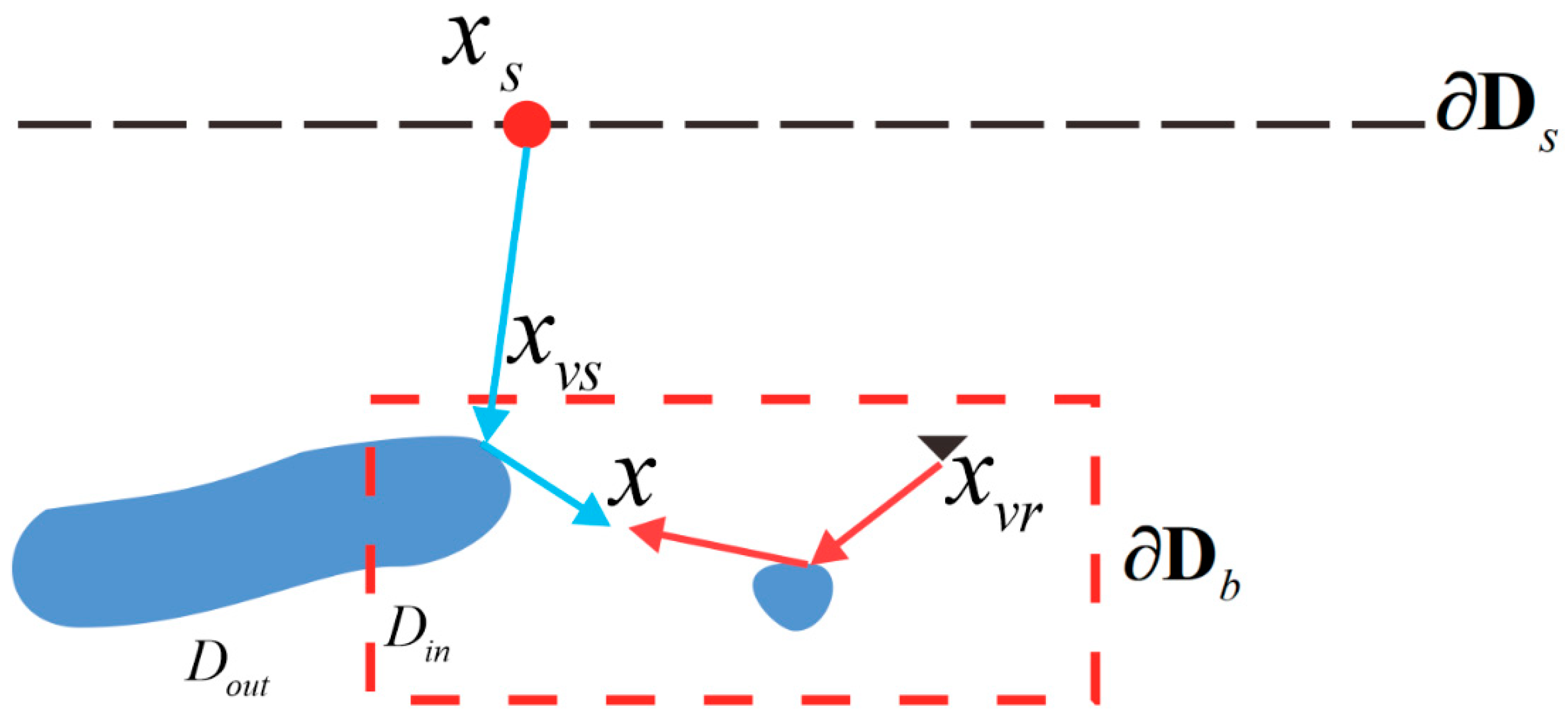
2.3. Marchenko Source-Receiver Redatuming with VSP Data

Based on the one-way reciprocity theorems of convolution and correlation [29], Singh and Snieder present the formula for the source-receiver Marchenko redatuming method [25]:

$$G^{-}({\mathrm{x}}_i,{\mathrm{x}}_j,\omega )={\displaystyle {\int }_{\partial D_s}2{(\iota \omega \rho ({\mathrm{x}}_s))}^{-1}{\partial }_{z}G({\mathrm{x}}_s,{\mathrm{x}}_j,\omega )f^{+}({\mathrm{x}}_s,{\mathrm{x}}_i,\omega )d{\mathrm{x}}_s},$$

(14)

and

$$G^{+}({\mathrm{x}}_i,{\mathrm{x}}_j,\omega )=-{\displaystyle {\int }_{\partial D_s}2{(\iota \omega \rho ({\mathrm{x}}_s))}^{-1}{\partial }_{z}G({\mathrm{x}}_s,{\mathrm{x}}_j,\omega )f^{-*}{({\mathrm{x}}_s,{\mathrm{x}}_i,\omega )}^{}d{\mathrm{x}}_s}.$$

(15)

where $\iota$ is the imaginary unit. $G({\mathrm{x}}_i,{\mathrm{x}}_j,\omega )$ is the Green’s function between the subsurface virtual source ${\mathrm{x}}_j$ and the subsurface virtual receiver ${\mathrm{x}}_i$. $G({\mathrm{x}}_s,{\mathrm{x}}_j,\omega )$ and $f^{\pm }({\mathrm{x}}_s,{\mathrm{x}}_i,\omega )$ on the right-hand side of Equations (14) and (15) can be calculated by the standard Marchenko Equations (12) and (13). However, as shown in Section 2.2, the Green’s function $G({\mathrm{x}}_s,{\mathrm{x}}_j,\omega )$ obtained by the standard Marchenko method may lack the laterally propagating waves.

VSP data $R_{VSP}({\mathrm{x}}_j,{\mathrm{x}}_s)$ is the signal at the receivers in the borehole. Compared to the redatumed Green’s function $G({\mathrm{x}}_s,{\mathrm{x}}_j)$ retrieved by the standard Marchenko method, the VSP data contain accurate laterally propagating wave information. The reciprocity theorem suggests that $R_{VSP}({\mathrm{x}}_j,{\mathrm{x}}_s)$ and $R_{VSP}({\mathrm{x}}_s,{\mathrm{x}}_j)$ are equivalent. This means that if we replace $G({\mathrm{x}}_s,{\mathrm{x}}_j,\omega )$ Equations (14) and (15) with $R_{VSP}({\mathrm{x}}_s,{\mathrm{x}}_j,\omega )$, we can obtain more accurate Green’s functions. Therefore, we can derive the formula of the Marchenko source-receiver redatuming method with VSP data [26]:

$$G({\mathrm{x}}_i,{\mathrm{x}}_j,\omega )={\displaystyle {\int }_{\partial D_s}2{(\iota \omega \rho ({\mathrm{x}}_s))}^{-1}{\partial }_z{R}_{VSP}({\mathrm{x}}_s,{\mathrm{x}}_j,\omega )(f^{+}({\mathrm{x}}_i,{\mathrm{x}}_s,\omega )-f^{+*}({\mathrm{x}}_i,{\mathrm{x}}_s,\omega ))d{\mathrm{x}}_s}.$$

(16)

It is important to note that Equations (14)–(16) need to satisfy the condition that ${\mathrm{x}}_i$ is above ${\mathrm{x}}_j$ in depth. In addition, due to the acquisition system of the VSP data, the positions of ${\mathrm{x}}_j$ are fixed (the positions of the receivers in the well). In other words, with Equation (16), we can obtain the accurate Green’s function between the virtual source at the locations of the receivers in the borehole and the virtual receivers at any points above the depth of that virtual source.

Similarly, we use the simple model in Section 2.2 as an example. Keeping the original acquisition system unchanged, the VSP receivers are set at depth intervals of 20 m in the well and at 2500 m in the X-direction. We estimate the Green’s function $G({\mathrm{x}}_j,{\mathrm{x}}_s)$ with an array of surface sources and a single subsurface virtual receiver at coordinates (X: 2500 m, Z: 5040 m) using the standard Marchenko receiver redatuming. Its comparison with the measured VSP signal $R_{VSP}({\mathrm{x}}_j,{\mathrm{x}}_s)$ is shown in Figure 4.

It can be clearly noticed from Figure 4 that the Green’s function $G({\mathrm{x}}_j,{\mathrm{x}}_s)$ obtained by the standard Marchenko receiver redatuming method lacks the lateral propagating wave components from diffractions compared to the actual measured VSP signal. Then, we also iteratively compute the focus function $f^{\pm }({\mathrm{x}}_i,{\mathrm{x}}_s,\omega )$ by the standard Marchenko method, where ${\mathrm{x}}_i$ (X: 3500 m; Z: 4170–5020 m) is an array of virtual receivers along the left vertical white line in Figure 1. We substitute $G({\mathrm{x}}_j,{\mathrm{x}}_s)$ and $R_{VSP}({\mathrm{x}}_j,{\mathrm{x}}_s)$, respectively, into Equation (16) to estimate the source-receiver redatumed Green’s functions $G({\mathrm{x}}_i,{\mathrm{x}}_j)$ between the virtual source ${\mathrm{x}}_j$ and virtual receivers ${\mathrm{x}}_i$. The results of the standard Marchenko source-receiver redatuming method and the Marchenko source-receiver redatuming with VSP data are shown in Figure 5. As a benchmark, Figure 5c shows the actual signal received by the ${\mathrm{x}}_i$ with the source at point ${\mathrm{x}}_j$.

It can be clearly noticed in Figure 5 that the standard Marchenko method cannot retrieve the laterally propagating wave components at the locations indicated by the red arrows. However, the VSP Marchenko method is consistent with the recorded signals. This proves that the results of the Marchenko method with VSP data can accurately reconstruct the lateral propagation waves. In the next section, we will describe how to incorporate the VSP Marchenko redatumed data into the local FWI process to improve the accuracy of the inversion results.

2.4. VSP-Driven Local FWI Method

Section 2.1 stated that when using only the standard Marchenko receiver redatuming method, we can only use the estimated signal between the surface sources and the virtual receivers at the top position of the target area as the observed data due to the inaccuracy of the lateral propagation wave redatuming. However, with the VSP Marchenko redatuming method, Green’s function can be obtained more accurately for the virtual receivers on the lateral side of the target, provided that the location of the virtual receivers is above the VSP receivers. Therefore, the VSP-driven local FWI requires only a simple substitution of the Green’s functions between VSP receivers and virtual receivers into the local FWI method. The array of VSP receiver points is denoted as ${\mathrm{x}}_{vsp}$. We calculate the Green’s functions $G_{all}^{mar}({\mathrm{x}}_{vs},{\mathrm{x}}_{vsp},\omega )$ and $G_{all}^{mar}({\mathrm{x}}_{vr}^{vsp},{\mathrm{x}}_{vsp},\omega )$ by the VSP Marchenko method. $P_{all}^{mar}({\mathrm{x}}_{vs},{\mathrm{x}}_{vsp},\omega )$ and $P_{all}^{mar}({\mathrm{x}}_{vr}^{vsp},{\mathrm{x}}_{vsp},\omega )$ are the wavefields of $G_{all}^{mar}({\mathrm{x}}_{vs},{\mathrm{x}}_{vsp},\omega )$ and $G_{all}^{mar}({\mathrm{x}}_{vr}^{vsp},{\mathrm{x}}_{vsp},\omega )$, then Equation (10) can be modified as follows,

$${\mathrm{F}}^{vsp}(m_{in},\omega )=\frac{1}{\iota \omega }{\displaystyle {\oint }_{\partial {\mathrm{D}}_b}\frac{1}{\rho ({\mathrm{x}}_{vs})}[G_{in}(\mathrm{x},{\mathrm{x}}_{vs},\omega )\frac{\partial }{\partial n_{{\mathrm{x}}_{vs}}}{P}_{all}^{mar}({\mathrm{x}}_{vs},{\mathrm{x}}_{vsp},\omega )-\frac{\partial }{\partial n_{{\mathrm{x}}_{vs}}}{G}_{in}(\mathrm{x},{\mathrm{x}}_{vs},\omega )P_{all}^{mar}({\mathrm{x}}_{vs},{\mathrm{x}}_{vsp},\omega )]}d{\mathrm{x}}_{vs}.$$

(17)

and Equation (11) can be written as,

$${\min }_{m_{in}}E(m_{in},\omega )=\frac{1}{2}{\displaystyle \sum _{{\mathrm{x}}_{vsp}}{‖{\mathbb{P}}_{vr}^{vsp}{\mathrm{F}}^{vsp}(m_{in},\omega )-P_{all}^{mar}({\mathrm{x}}_{vr}^{vsp},{\mathrm{x}}_{vsp},\omega )‖}_2^2}.$$

(18)

It should be noted that ${\mathbb{P}}_{vr}^{vsp}$ in Equation (18) is different from ${\mathbb{P}}_{vr}^{}$ in Equation (11). The differences are shown in Figure 6. The capability of including the laterally propagating waves from the VSP Marchenko source-receiver redatuming method allows the improvement of the lateral resolution for the inversion. Therefore, ${\mathbb{P}}_{vr}^{vsp}$ is set mainly vertically on the lateral side of the target.

By combining Equations (11) and (18), the objective function of the VSP and Surface data jointed local FWI method can be written as:

$${\min }_{m_{in}}E(m_{in},\omega )=\frac{1}{2}{\displaystyle \sum _{{\mathrm{x}}_s}{‖{\mathbb{P}}_{vr}\mathrm{F}(m_{in},\omega )-P_{all}^{mar}({\mathrm{x}}_{vr},{\mathrm{x}}_s,\omega )‖}_2^2}+\frac{1}{2}\alpha {\displaystyle \sum _{{\mathrm{x}}_{vsp}}{‖{\mathbb{P}}_{vr}^{vsp}{\mathrm{F}}^{vsp}(m_{in},\omega )-P_{all}^{mar}({\mathrm{x}}_{vr}^{vsp},{\mathrm{x}}_{vsp},\omega )‖}_2^2}.$$

(19)

where $\alpha$ is a weighting factor to balance the residuals and gradients of the two terms on the right side of the equation. In the general case, the quantities of ${\mathrm{x}}_s$ and ${\mathrm{x}}_{vsp}$ differ significantly and the redatumed wavefields $P_{all}^{mar}({\mathrm{x}}_{vr},{\mathrm{x}}_s)$ and $P_{all}^{mar}({\mathrm{x}}_{vr}^{vsp},{\mathrm{x}}_{vsp})$ also differ in energy, so that $\alpha$ is necessary. The gradient of Equation (19) can be easily calculated using the adjoint state method [27]. The gradient of Equation (19) can be expressed as:

$$\delta E={\displaystyle \sum _{{\mathrm{x}}_s}{\omega }^2}diag{(\mathrm{F}(m_{in},\omega ))}^{*}{v}_{in}+\alpha {\displaystyle \sum _{{\mathrm{x}}_{vsp}}{\omega }^2}diag{({\mathrm{F}}^{vsp}(m_{in},\omega ))}^{*}{v}_{in}^{vsp}.$$

(20)

The $v_{in}$ and $v_{in}^{vsp}$ are the local adjoint wavefields in the target volume corresponding to the surface source ${\mathrm{x}}_s$ and the virtual source ${\mathrm{x}}_{vsp}$, respectively. Local adjoint wavefields can be obtained as follows:

$$A(m_{in},\omega )v_{in}={\mathbb{P}}_{vr}^T({\mathbb{P}}_{vr}^{}\mathrm{F}(m_{in},\omega )-P_{all}^{mar}({\mathrm{x}}_{vr},{\mathrm{x}}_s,\omega )),$$

(21)

and

$$A(m_{in},\omega )v_{in}^{vsp}={({\mathbb{P}}_{vr}^{vsp})}^T({\mathbb{P}}_{vr}^{vsp}{\mathrm{F}}^{vsp}(m_{in},\omega )-P_{all}^{mar}({\mathrm{x}}_{vr}^{vsp},{\mathrm{x}}_{vsp},\omega )).$$

(22)

Finally, the commonly used L-BFGS quasi-Newton algorithm is used to iteratively calculate the updates of target local model parameters.

3. Example

To clearly describe the computational process and effectiveness of the method, a 3D model of the strike-slip faulted and fracture-vuggy carbonate reservoir in the Tarim Basin is used as an example. The 3D model of the strike-slip faulted, and fracture-vuggy carbonate reservoir in Tarim Basin is based on the typical characteristics of slip-faulted and karst reservoirs in the field, which is a benchmark model (similar to the Marmousi model). One shot line in the synthesized 3D acquisition record is used for our test. The 2D profile of the benchmark model depth range is 0 to 7900 m, and the X-direction range is 0 to 6600 m (Figure 7a). A total of 281 shots at the surface with an 80 m shot interval is acquired. The source is a Ricker wavelet with a 25 Hz peak frequency. For surface seismic data, each shot corresponds to 241 receivers at the surface with a 40 m receiver interval. There are 35 VSP receivers fixed in the well at 2500 m in the X-direction with a 20 m vertical interval from depths of 6300 m to 7000 m, and the range of local FWI is the area enclosed by the white color rectangle in Figure 7a. The migration velocity model is used as the initial model (Figure 7b). The reverse time migration imaging profile are shown in Figure 7c.

Due to the laterally interfering seismic response, there is only one wider “beam string” reflection in the imaging profile. The two caves in the lateral direction are completely unidentifiable. Its low lateral resolution causes interpretation uncertainty. Such errors in reservoir identification can pose a significant risk to the design of the trajectories of wells in drilling development. We apply local full waveform inversion to the target region to verify whether the method can accurately restore the fine scale model structure.

First, we need to estimate the required Green’s functions using the standard Marchenko method. The standard Marchenko receiver redatuming with a virtual receiver array location at ${\mathrm{x}}_{vr}$ = (X: 2155–4145 m, Z: 5555 m) corresponding to a surface source at ${\mathrm{x}}_s$ = (X: 3150 m, Z: 0 m), is tested. The virtual receiver location array is shown by the black solid line in Figure 7d. The wavefield $P_{all}^{mar}({\mathrm{x}}_{vr},{\mathrm{x}}_s)$ of the retrieved Green’s function $G_{all}^{mar}({\mathrm{x}}_{vr},{\mathrm{x}}_s)$ is shown in Figure 8a and can be compared with the wavefield signal (Figure 8b) obtained by waveform modeling with the true velocity model. The comparison in Figure 8 shows that most reflection events are reconstructed relatively well and that the redatumed Green’s function satisfies the need for inversion.

Second, we use the VSP Marchenko source-receiver redatuming to retrieve the Green’s function $G_{all}^{mar}({\mathrm{x}}_{vr}^{vsp},{\mathrm{x}}_{vsp})$ and its corresponding wavefield. The virtual receiver locations of this method are shown in Figure 7d, where the virtual source (VSP receiver point) is located at ${\mathrm{x}}_{vsp}$ = (X: 2500 m, Z: 6600 m) and the virtual receiver array location at ${\mathrm{x}}_{vr}^{vsp}$ = (X: 2155 m, Z: 5555–6185 m) is shown by the left black dashed line. The wavefield $P_{all}^{mar}({\mathrm{x}}_{vr}^{vsp},{\mathrm{x}}_{vsp})$ of the retrieved Green’s function $G_{all}^{mar}({\mathrm{x}}_{vr}^{vsp},{\mathrm{x}}_{vsp})$ is shown in Figure 9a and can be compared with the wavefield signal (Figure 9b) obtained by waveform modeling with the true velocity model. Benefiting from the incorporation of VSP data, the errors between the redatumed wavefield and the full wavefield are very small. The laterally propagating waves caused by strike-slip faulting and cavities are accurately reconstructed. It should be noted that all the events before the arrival of the direct wave in redatumed signals need to be muted in further calculations. Since $G_{all}^{mar}({\mathrm{x}}_{vs},{\mathrm{x}}_s)$ and $G_{all}^{mar}({\mathrm{x}}_{vs},{\mathrm{x}}_{vsp})$ are obtained in the same manner as $G_{all}^{mar}({\mathrm{x}}_{vr},{\mathrm{x}}_s)$ and $G_{all}^{mar}({\mathrm{x}}_{vr}^{vsp},{\mathrm{x}}_{vsp})$, we will not repeat it here.

In the standard Marchenko receiver redatuming-based local FWI, a total of 45 surface sources at ${\mathrm{x}}_s$ = (X: 1200–4800 m; Z: 0 m) above the target area are used in the calculation, while the VSP-driven local FWI also contains 35 subsurface sources at ${\mathrm{x}}_{vsp}$ = (X: 2500 m; Z: 6300–7000 m). Starting from the target region of the smooth velocity model in Figure 7b, the minimum frequency of the inversion is 8 Hz, the maximum frequency is 44 Hz, and the step size of the frequency is 2 Hz. To sharpen the inversion results, we use the minimum support regularization as a constraint. It should be noted that in this example, the weighting factor $\alpha$ is 1 because the number of VSP virtual sources and surface sources in the inversion are similar and the energy is also balanced. The results of the local FWI based on the standard Marchenko redatuming are shown in Figure 10a. The result of the VSP and Surface data jointed local FWI is shown in Figure 10b. For reference, we also replaced the standard Marchenko retrieved signals with the corresponding measurement signals to perform local FWI, and the result is shown in Figure 10c. From Figure 10b, the cavity boundaries are well characterized to match the true model. Compared with Figure 10a, the inverted model in Figure 10b has a better lateral resolution, and the two cavities are clearly separated, while the strike-slip fault with a steep dip angle can be reconstructed. The result of VSP and Surface data jointed local FWI still has certain errors for the characterization of the strike-slip fault compared to Figure 10c, and it is mainly due to the mismatches in the redatumed Green’s function caused by the deep depth of the target area and the limited acquisition aperture.

The comparison of the lateral model single trace at a depth of 5.85 km is shown in Figure 11, which can more clearly demonstrate the difference in lateral resolution and accuracy of the inversion results of different methods. Especially in cavity reservoir locations with low impedance, the results of the standard Marchenko method of local full waveform inversion cannot reconstruct accurate parameter values. The inversion result of the VSP and surface data jointed local FWI looks closer to the actual model.

4. Discussion

We demonstrate the feasibility of the proposed VSP-driven local FWI for improving the lateral resolution of inverted results of standard Marchenko local FWI and effectively improving the reconstruction of steep structures. Characterizing reservoirs using traditional full waveform inversion methods is difficult, especially when the reservoir is deeply buried. The benchmark model of the Tarim Basin in the example chapter has a high-velocity layer caused by igneous rocks at a depth of 2.7 km, and the strong reflection caused by the high-velocity layer will repress the signal of the deep target layer, which leads to an inaccurate result of conventional FWI for the deep layer (Figure 12).

By comparing Figure 10a with Figure 12, it can be seen that local FWI based on the standard Marchenko method has a very significant improvement compared to full-domain FWI for the same number of iterations. This is due to the fact that local FWI is oriented to local gradients and eliminates the influence of the overburden. However, the lateral resolution in Figure 10a still cannot fully distinguish between the two caves, while the strike-slip fault cannot be accurately reconstructed either due to the aperture limitation. In the present study, our proposed VSP-driven local full-waveform inversion and joint local full-waveform inversion enhance the lateral variation of the gradients by adding lateral observations. Figure 13 shows that the gradient of the VSP-driven local FWI term mainly as a contribution to the lateral variation. The advantage of this method is that the accurate laterally propagating waves can be obtained by Marchenko source-receiver redatuming with VSP data, which results in a higher lateral resolution for the inverted model. In Figure 10b, the lateral resolution of the two caves is improved compared to that in Figure 10a, while the strike-slip faults are also inverted. In particular, this method has great potential for identifying small-scale stratigraphic lateral discontinuities and distributed geological objects.

As the extension of local FWI based on the Marchenko redatuming method, VSP and Surface data jointed local FWI also has computational efficiency. The computation time of both methods in the inversion process is basically the same, but VSP-driven local FWI needs to retrieve more redatumed subsurface wavefields. It will take more time in the data preparation process (compared to the standard Marchenko receiver redatuming requires the additional process of calculating Equation (16)), but it is still much more efficient than full model domain FWI.

However, there are still issues with the proposed method. This paper presents the Marchenko source-receiver redatuming with the requirement that the virtual receiver is above the virtual source [25]. Both the focusing and Green’s functions can be calculated at every point. The Green’s functions can be calculated between any two points when both input fields are Marchenko estimates [26]. However, the VSP data as actual observations of the receivers in the well lead to the situation that when using the VSP Marchenko source-receiver redatuming method, we can only estimate the Green’s function between a virtual source at a location of the VSP receiver to an arbitrary point above it. This limits the application of the VSP-driven local FWI. At the same time, in the case of vertical structures such as faults, a large aperture is required to ensure that the primary amplitude reflected from the vertical structure can be measured at the surface. In other words, to perform VSP Marchenko source-receiver redatuming to obtain the exact Green’s function containing the laterally propagating waves also requires certain aperture conditions. We reduce the surface shot records used for the Marchenko redatuming in the example chapter to 105 shots (X: −1000 m–7400 m) and recalculate the Green’s function. The common VSP virtual source gather is shown in Figure 14. Compared with Figure 9a, the retrieval accuracy of the laterally propagating waves receives a larger impact with the reduction of the aperture. The main reason for the current limitation of local full waveform inversion mainly depends on the accuracy of the redatumed wavefield, and more exploration in this direction is needed in the future. In addition, considering the viscoelastic behavior of subsurface in petroleum exploration is crucial because viscoelastic inversion is highly sensitive to fluid content due to the energy losses caused by their viscosity [30,31]. This sensitivity is explained by viscous fluid flow during the passage of the waves, which causes frictional movement at the grain surfaces [32,33]. The physical complexity of FWI models can be overcome by incorporating machine-learning models [34]. Therefore, incorporating the viscoelasticity and machine learning models in local FWI may significantly enhance seismic imaging and interpretation in reservoir zones, which is the direction of our future research.

5. Conclusions

In this paper, we developed a VSP-driven local full waveform inversion. First of all, we demonstrate the local FWI based on the standard Marchenko redatuming. We then introduced the Marchenko source-receiver redatuming method with VSP data to estimate the subsurface redatumed wavefield containing more accurate laterally propagating waves. A numerical experiment was carried out to investigate the sensitivities of the VSP Marchenko source-receiver redatuming method and the standard Marchenko redatuming method to laterally propagating waves. The VSP-driven local FWI can be performed by simply reforming the objective function of the local FWI based on standard Marchenko redatuming.

The VSP and surface data jointed local FWI was applied to a synthetic data set of the Benchmark model of the strike-slip faulted and fracture-vuggy carbonate reservoir in Tarim Basin. As a result of the inclusion of laterally propagating waves in the observed data, the VSP and surface data jointed local FWI has a significant improvement in the lateral resolution of small structures compared to local FWI based on standard Marchenko redatuming.

References

1. Gray, S.H.; Etgen, J.; Dellinger, J.; Whitmore, D. Seismic migration problems and solutions. Geophysics 2001, 66, 1622–1640. [Google Scholar] [CrossRef]
2. Landa, E. Seismic diffraction: Where’s the value? In SEG Technical Program Expanded Abstracts; Society of Exploration Geophysicists: Las Vegas, NV, USA, 2012. [Google Scholar] [CrossRef]
3. Decker, L.; Janson, X.; Fomel, S. Carbonate reservoir characterization using seismic diffraction imaging. Interpretation 2015, 3, 21–30. [Google Scholar] [CrossRef]
4. Tarantola, A. Inversion of seismic reflection data in the acoustic approximation. Geophysics 1984, 49, 1259–1266. [Google Scholar] [CrossRef]
5. Tarantola, A. A strategy for nonlinear elastic inversion of seismic reflection data. Geophysics 1986, 51, 1893–1903. [Google Scholar] [CrossRef]
6. Pratt, R.G. Seismic waveform inversion in the frequency domain, Part 1: Theory and verification in a physical scale model. Geophysics 1999, 64, 659–992. [Google Scholar] [CrossRef] [Green Version]
7. Ben-Hadj-Ali, H.; Operto, S.; Virieux, J. Velocity model building by 3D frequency-domain, full-waveform inversion of wide-aperture seismic data. Geophysics 2008, 73, 101–117. [Google Scholar] [CrossRef] [Green Version]
8. Takougang, E.M.T.; Ali, M.Y.; Bouzidi, Y.; Bouchaala, F.; Sultan, A.A.; Mohamed, A.I. Characterization of a carbonate reservoir using elastic full-waveform inversion of vertical seismic profile data. Geophys. Prospect. 2020, 68, 1944–1957. [Google Scholar] [CrossRef]
9. Lu, R. Revealing overburden and reservoir complexity with high-resolution FWI. In SEG Technical Program Expanded Abstracts; Society of Exploration Geophysicists: Dallas, TX, USA, 2016. [Google Scholar] [CrossRef]
10. Alford, R.M.; Kelly, K.R.; Boore, D.M. Accuracy of finite-difference modeling of the acoustic wave equation. Geophysics 1974, 39, 834–842. [Google Scholar] [CrossRef] [Green Version]
11. Routh, P.; Neelamani, R.; Lu, R.; Lazaratos, S.; Braaksma, H.; Hughes, S.; Saltzer, R.; Stewart, J.; Naidu, K.; Averill, H.; et al. Impact of high-resolution FWI in the Western Black Sea: Revealing overburden and reservoir complexity. Lead. Edge 2017, 36, 60–66. [Google Scholar] [CrossRef]
12. Yuan, S.; Fuji, N.; Singh, S.; Borisov, D. Localized time-lapse elastic waveform inversion using wavefield injection and extrapolation: 2-D parametric studies. Geophys. J. Int. 2017, 209, 1699–1717. [Google Scholar] [CrossRef]
13. Yuan, S.; Fuji, N.; Singh, S. High-frequency localized elastic full-waveform inversion for time-lapse seismic surveys. Geophysics 2021, 86, 277–292. [Google Scholar] [CrossRef]
14. Cui, T.; Rickett, J.; Vasconcelos, I.; Veitch, B. Target-oriented full-waveform inversion using Marchenko redatumed wavefields. Geophys. J. Int. 2020, 223, 792–810. [Google Scholar] [CrossRef]
15. Guo, Q.; Alkhalifah, T. Target-oriented waveform redatuming and high-resolution inversion: Role of the overburden. Geophysics 2020, 85, 525–536. [Google Scholar] [CrossRef]
16. Robertsson, J.O.; Chapman, C.H. An efficient method for calculating finite-difference seismograms after model alterations. Geophysics 2020, 65, 907–918. [Google Scholar] [CrossRef]
17. Guo, Q.; Alkhalifah, T. Target-oriented inversion with least-squares waveform redatuming. In SEG Technical Program Expanded Abstracts; Society of Exploration Geophysicists: San Antonio, TX, USA, 2019. [Google Scholar] [CrossRef]
18. Li, Y.; Alkhalifah, T. Target-oriented high-resolution elastic full-waveform inversion with an elastic redatuming method. Geophysics 2022, 87, 379–389. [Google Scholar] [CrossRef]
19. Wapenaar, K.; Broggini, F.; Slob, E.; Snieder, R. Three-dimensional single-sided Marchenko inverse scattering, data-driven focusing, Green’s function retrieval, and their mutual relations. Phys. Rev. Lett. 2013, 110, 084301. [Google Scholar] [CrossRef] [Green Version]
20. Wapenaar, K.; Slob, E. On the Marchenko equation for multicomponent single-sided reflection data. Geophys. J. Int. 2014, 199, 1367–1371. [Google Scholar] [CrossRef] [Green Version]
21. Slob, E.; Wapenaar, K.; Broggini, F.; Snieder, R. Seismic reflector imaging using internal multiples with Marchenko-type equations. Geophysics 2014, 79, 63–76. [Google Scholar] [CrossRef] [Green Version]
22. van der Neut, J.; Vasconcelos, I.; Wapenaar, K. On Green’s function retrieval by iterative substitution of the coupled Marchenko equations. Geophys. J. Int. 2015, 203, 792–813. [Google Scholar] [CrossRef]
23. Chen, X.; Hu, Y.; Huang, X.; Zhang, H.; Xu, Y.; Tang, J. Marchenko imaging based on self-adaptive traveltime updating. Appl. Geophys. 2020, 17, 81–91. [Google Scholar] [CrossRef]
24. Edinburgh, K.W.; van der Neut, J. Marchenko redatuming: Advantages and limitations in complex media. In Proceedings of the 15th International Congress of the Brazilian Geophysical Society & EXPOGEF, Rio de Janeiro, Brazil, 31 July–3 August 2017. [Google Scholar] [CrossRef] [Green Version]
25. Singh, S.; Snieder, R. Source-receiver Marchenko redatuming: Obtaining virtual receivers and virtual sources in the subsurface. Geophysics 2017, 82, 13–21. [Google Scholar] [CrossRef] [Green Version]
26. Lomas, A.; Singh, S.; Curtis, A. Imaging vertical structures using Marchenko methods with vertical seismic-profile data. Geophysics 2020, 85, 103–113. [Google Scholar] [CrossRef]
27. Plessix, R.E. A review of the adjoint-state method for computing the gradient of a functional with geophysical applications. Geophys. J. Int. 2006, 167, 495–503. [Google Scholar] [CrossRef]
28. Wapenaar, K.; Fokkema, J. Green’s function representations for seismic interferometry. Geophysics 2006, 71, 33–46. [Google Scholar] [CrossRef]
29. Wapenaar, K. Reciprocity properties of one-way propagators. Geophysics 1998, 63, 1795–1798. [Google Scholar] [CrossRef] [Green Version]
30. Gao, L.; Pan, Y.; Rieder, A.; Bohlen, T.; Mao, W. Multiparameter 2-D viscoelastic full-waveform inversion of Rayleigh waves: A field experiment at Krauthausen test site. Geophys. J. Int. 2023, 234, 297–312. [Google Scholar] [CrossRef]
31. Matsushima, J.; Ali, M.Y.; Bouchaala, F. A novel method for separating intrinsic and scattering attenuation for zero-offset vertical seismic profiling data. Geophys. J. Int. 2017, 211, 1655–1668. [Google Scholar] [CrossRef]
32. Bouchaala, F.; Ali, M.Y.; Farid, A. Estimation of compressional seismic wave attenuation of carbonate rocks in Abu Dhabi. C. R. Geosci. 2014, 346, 169–178. [Google Scholar] [CrossRef]
33. Müller, T.M.; Gurevich, B.; Lebedev, M. Seismic wave attenuation and dispersion resulting from wave-induced flow in porous rocks—A review. Geophysics 2010, 75, 75A147–75A164. [Google Scholar] [CrossRef]
34. Singh, S.; Tsvankin, I.; Naeini, E.Z. Elastic FWI for orthorhombic media with lithologic constraints applied via machine learning3D elastic orthorhombic FWI. Geophysics 2021, 86, R589–R602. [Google Scholar] [CrossRef]
Figure 1. Schematic of Green’s function in different computational states. Blue arrows mean the Green’s function between the surface source x s and a point in the target area x in the medium state of the full-domain model. Red arrows mean the Green’s function between x and a virtual receiver x v r in the truncated medium state.
Applsci 13 04165 g001
Figure 2. A simple model and the target zone (area enclosed by the solid white lines). VSP receivers are set along the black dotted line at 2500 m in the X direction.
Applsci 13 04165 g002
Figure 3. Wavefield snapshots of the target zone at time 1.64 s with a surface source at 4 km in X direction obtained by standard Marchenko redatuming (a) and forward modeling (b).
Applsci 13 04165 g003
Figure 4. The common receiver gathers corresponding to the virtual receiver (VSP receiver) at x j (X: 2500 m; Z: 5040 m). From (a), the standard Marchenko receiver redatuming method retrieved wavefield of Green’s function G ( x j , x s ) ; from (b), the measurement VSP data from direct modeling.
Applsci 13 04165 g004
Figure 5. A comparison of wavefields of the retrieved Green’s functions between a virtual source (X: 2500 m; Z: 5040 m) and virtual receivers (X: 3500 m; Z: 4170–5020 m) based on different methods. (a) The estimated wavefield using the standard Marchenko source-receiver redatuming. (b) The estimated wavefield using the Marchenko source-receiver redatuming with VSP data. (c) The waveform modeling result based on the true model.
Applsci 13 04165 g005
Figure 6. Schematics of the location of the virtual receivers in the local FWI based on the standard Marchenko receiver redatuming (a) and the VSP-driven local FWI (b). The internal part of the area surrounded by the rectangle of red dots is the target zone. The red dots represent the virtual source points x v s , the green dots are the virtual receiver points x v r (a) and x v r v s p (b), the blue dots are the physical surface sources x s , and the pink dots are the subsurface VSP receivers x v s p . The black dots are other grid points within the target volume.
Applsci 13 04165 g006
Figure 7. The 2D profile of the Benchmark model (a), the initial model for migration (b), the RTM imaging (c), and the target zone of the true model (d). The black solid line in subfigure (d) indicates the setting location of virtual receivers x v r in standard Marchenko local FWI. The black dashed lines indicate the setting location of virtual receivers x v r v s p in VSP-driven Marchenko local FWI. The black dashed line is the well location. And the white color rectangle is the target region.
Applsci 13 04165 g007
Figure 8. The common source gathers with a row of virtual receivers x v r = (X: 2155–4145 m, Z: 5555 m) corresponding to the surface source at 3150 m in X-coordinate from (a) the standard Marchenko receiver redatuming method retrieved wavefield and (b) the wavefield obtained by waveform modeling.
Applsci 13 04165 g008
Figure 9. The common source gathers with a column of virtual receivers x v r = (X: 2155 m, Z: 5555–6185 m) corresponding to a virtual source at x v s p = (X: 2500 m, Z: 6600 m) from (a) the Marchenko source-receiver redatuming with VSP data retrieved wavefield and (b) wavefield obtained by waveform modeling.
Applsci 13 04165 g009
Figure 10. Comparison of local FWI results using different methods with (a) local FWI based on standard Marchenko receiver redatuming. (b) VSP and surface data jointed local FWI based on VSP data jointed Marchenko source-receiver redatuming. (c) Local FWI using modeling subsurface wavefield as a reference. (d) True local model as a benchmark.
Applsci 13 04165 g010
Figure 11. Comparison of velocity lateral profile from true model and inverted models using different methods.
Applsci 13 04165 g011
Figure 12. The inversion result of conventional full-domain FWI.
Applsci 13 04165 g012
Figure 13. Gradient comparison of VSP-driven local FWI term (a) and surface data local FWI term (b) at 30 Hz frequency.
Applsci 13 04165 g013
Figure 14. The common source gather with a column of virtual receivers x v r = (X: 2155 m, Z: 5555–6185 m) corresponding to a virtual source at x v s p = (X: 2500 m, Z: 6600 m) obtained by the VSP Marchenko source-receiver redatuming with a small aperture.
Applsci 13 04165 g014
Disclaimer/Publisher’s Note: The statements, opinions and data contained in all publications are solely those of the individual author(s) and contributor(s) and not of MDPI and/or the editor(s). MDPI and/or the editor(s) disclaim responsibility for any injury to people or property resulting from any ideas, methods, instructions or products referred to in the content.